Embed Size (px)
Citation preview
Why Does Return Predictability Concentrate in Bad
Times?∗
Julien Cujean† Michael Hasler‡
November 20, 2014
Abstract
We build an equilibrium model to explain why stock return predictability is con-
centrated in bad times. The key ingredient is countercyclical investors’ disagreement,
which originates from heterogeneous models. As economic conditions deteriorate, dif-
ference in investors’ learning speed increases, disagreement spikes and returns react
to past news. The model explains several findings: the link between disagreement
and future returns, time-series momentum and how it crashes after sharp market re-
bounds, and investors’ superior performance in bad times. The model further predicts
that time-series momentum is related positively to disagreement and negatively to eco-
nomic conditions. We provide empirical support to these new predictions.
Keywords. Equilibrium Asset Pricing, Learning, Disagreement, Business Cycle, Pre-
dictability, Times-Series Momentum, Momentum Crashes.
JEL Classification. D51, D83, G12, G14.
∗We would like to thank Hui Chen, Peter Christoffersen, Pierre Collin-Dufresne, Michel Dubois, Dar-rell Duffie, Bernard Dumas, Laurent Fresard, Steve Heston, Julien Hugonnier, Alexandre Jeanneret, ScottJoslin, Andrew Karolyi, Leonid Kogan, Jan-Peter Kulak, Pete Kyle, Jeongmin Lee, Mark Loewenstein, Se-myon Malamud, Erwan Morellec, Antonio Mele, Lubos Pastor, Lasse Pedersen, Remy Praz, Alberto Rossi,Rene Stulz, Adrien Verdelhan, Pietro Veronesi, Jason Wei, Liyan Yang, and seminar participants at the4th Financial Risks International Forum, Collegio Carlo Alberto, Goethe University Frankfurt, SFI-NCCRWorkshop, University of California at San Diego, University of Geneva, University of Maryland, Universityof Neuchatel, and University of Toronto for their insightful comments. Financial support from the Univer-sity of Maryland and the University of Toronto is gratefully acknowledged. A previous version of this papercirculated under the title “Time-Series Predictability, Investors’ Disagreement, and Economic Conditions”.†University of Maryland, Robert H. Smith School of Business, 4466 Van Munching Hall, College Park,
MD 20742, USA; +1 (301) 405 7707; [email protected]; www.juliencujean.com‡University of Toronto, Rotman School of Management, 105 St. George Street, Toronto, ON, M5S 2E8,
Canada; +1 (416) 946 8494; [email protected]; www.rotman.utoronto.ca/Hasler
1 Introduction
Investors’ disagreement (Diether, Malloy, and Scherbina, 2002) and the content of news
(Tetlock, 2007) predict future returns. Recent evidence further suggests that stock return
predictability using investors’ disagreement (Cen, Wei, and Yang, 2014) and the content of
news (Garcia, 2013) is concentrated in bad times.1 Yet, the mechanism that causes return
predictability to vary over the business cycle remains unclear.
In this paper, we provide an explanation why investors’ disagreement and news’ content
better predict future returns in bad times. We base our explanation on the empirical finding
that disagreement among professional forecasters originates from heterogeneity in models and
moves countercyclically (Patton and Timmermann, 2010).2 The main idea is that investors
learn at different speeds. Some investors focus on sharp variations in the business cycle and
are “fast learners”, while others focus on long-term fluctuations and are “slow learners”. As
economic conditions deteriorate, the difference in learning speeds increases and disagreement
spikes, causing prices to continue to react to past news. Return predictability therefore
concentrates in bad times.
We introduce model heterogeneity within a dynamic general equilibrium populated with
two investors, A and B. Investors trade one stock and a riskless bond and consume the divi-
dends that the stock pays out. Agents do not observe the expected growth rate of dividends,
which we call the fundamental, and have different views regarding the empirical process
that governs it. Agent A focuses on long-term fundamental variations and assumes that the
economy transits smoothly from good to bad times. In contrast, Agent B focuses on short-
term fundamental fluctuations and postulates that the economy may transit precipitously
from good to bad times.3 Although investors observe the same information (past dividend
realizations), they disagree about the fundamental because they use different models and
therefore interpret the data differently.
1See also Loh and Stulz (2014) for similar evidence related to revisions in analysts’ forecasts.2Kandel and Pearson (1995) also show that disagreement stems from model heterogeneity and Veronesi
(1999), Carlin, Longstaff, and Matoba (2013), and Barinov (2014) provide empirical evidence of counter-cyclical disagreement.
3Agent A’s model follows a mean-reverting process (Detemple (1986, 1991), Wang (1993), Brennan andXia (2001), Scheinkman and Xiong (2003), Bansal and Yaron (2004), and Dumas, Kurshev, and Uppal(2009)), while Agent B’s model follows a Markov switching process (David (1997, 2008), Veronesi (1999,2000), Chen (2010), Bhamra, Kuehn, and Strebulaev (2010), and David and Veronesi (2013)).
1
The mechanism through which investors learn may differ significantly depending on eco-
nomic conditions, leading to a pattern of disagreement that changes over the business cycle.4
In good times, investors adjust their expectations at comparable speeds and disagreement
exhibits little variation. Difference in adjustment speeds between Agents A and B becomes
apparent in normal times. While agents expect the economy to move in the same direc-
tion, Agent B—the fast learner—adjusts her expectations significantly faster than Agent
A. This difference in learning speeds exacerbates disagreement in the short-term. In bad
times, model heterogeneity implies that investors expect the economy to move in opposite
directions. This polarization of opinions produces a large spike in disagreement.5
Countercyclical spikes in disagreement cause return predictability to be concentrated
in bad times. To see this, suppose there is a positive news shock today. In bad times,
the news polarizes opinions: while Agent A revises her expectations upwards, Agent B
revises her expectations downwards. Agent B’s pessimism in turn generates a persistent and
negative price reaction to the news shock in the short term, similar to the under-reaction
phenomenon of Jegadeesh and Titman (1993). In normal times, the news exacerbates the
difference in adjustment speeds, precipitating an upward revision in Agent B’s expectations.
Agent B’s overreaction relative to Agent A in turn gives rise to a persistent and positive price
reaction to the news shock in the short term, similar to the over-reaction phenomenon of
De Bondt and Thaler (1985). In the long term, agents’ opinions align, leading to a reversion
to fundamentals. In good times, predictability vanishes because the news generates little
disagreement and reversion to fundamentals therefore occurs instantly.
Price continuation in bad and normal times produces time-series momentum in excess
returns (Moskowitz, Ooi, and Pedersen, 2012). Consistent with empirical findings, returns
exhibit momentum over a one-year horizon and then revert over subsequent horizons (due
to reversion to fundamentals). Moreover, the term structure of returns’ serial correlation is
hump shaped: momentum is strong at short horizons and decays at intermediate horizons.
Importantly, at short horizons, time-series momentum is strongest in bad times. The reason
4In our paper, learning asymmetries arise across agents because agents use different models. In anothercontext, Chalkley and Lee (1998), Veldkamp (2005), and Van Nieuwerburgh and Veldkamp (2006) also obtainasymmetries in learning over the business cycle. Yet, the reason is that the information flow fluctuates witheconomic conditions.
5These dynamics of disagreement are consistent with those observed empirically (Patton and Timmer-mann (2010)). Moreover, they arise naturally as we let agents calibrate their own model to historical data.
2
is that the polarization of opinions in bad times, as opposed to the difference in adjustment
speeds in normal times, leads to a sharper spike in disagreement. By contrast, in good
times, excess returns exhibit strong reversal at short horizons. An important consequence
of this reversal spike is that a time-series momentum strategy may crash after sharp market
rebounds.6 Sharp trend reversals typically occur at the end of financial crises. For instance,
a time-series momentum crash occurred in March 2009.
We provide empirical support to two new predictions of the model. In particular, our
model predicts that time-series momentum is (1) strongest at short horizons in bad times
and (2) increasing in investors’ disagreement. We show that, over the last century, time-
series momentum at a one-month lag is significantly stronger during recessions—momentum
profits are, on average, twice as large in recessions as they are in expansions—consistent
with the first prediction of the model. Second, we find that time-series momentum increases
with the dispersion of analysts’ forecasts, a finding that supports the second prediction of
the model.
The model has additional implications for investors’ trading strategies and profits, as well
as trading volume. First, regarding the long-term investor (Agent A) as a mutual fund, our
model reconciles two empirical findings: mutual funds generate larger profits in bad times7
(Moskowitz, 2000) and focus on market-timing strategies during recessions8 (Kacperczyk, van
Nieuwerburgh, and Veldkamp, 2013). Indeed, the long-term investor trades on momentum
in bad and normal times and reverts her strategy in good times to avoid momentum crashes.
Doing so, she reaps large profits in bad times, precisely when short-term predictability is
strongest, and little profits in good times, when predictability vanishes. Finally, we show
that trading volume is countercyclical (Karpoff, 1987) and therefore positively related to
momentum (Lee and Swaminathan, 2000).
This paper contributes to two strands of literature. First, there is a vast literature on
heterogeneous beliefs. This literature focuses, to a large extent, on volatility, risk premium,
trading volume and bubbles, among other implications of investors’ disagreement.9 Our fo-
6Daniel and Moskowitz (2013) and Barroso and Santa-Clara (2014) document the occurrence of cross-sectional momentum crashes. Moskowitz et al. (2012) document a similar phenomenon in the time-series ofreturns.
7See also Glode (2011), Kosowski (2011), and Lustig and Verdelhan (2010).8Ferson and Schadt (1996) provide evidence that fund managers timing ability varies with economic
conditions. Dangl and Halling (2012) show that market-timing strategies work best in recessions.9See Xiong (2014) for a literature review.
3
cus, instead, is on the time-series predictability of stock returns. Moreover, in this literature,
the dynamics of disagreement are specific to the source of heterogeneous beliefs considered.10
In contrast with the literature, investors in this paper disagree because they use different
models (an Ornstein-Uhlenbeck process and a Markov chain). The resulting pattern of dis-
agreement has distinct implications for the predictability of stock returns. In particular, the
large difference in adjustment speeds across agents and the polarization of their opinions—
which do not arise together with other specifications in the literature—generate counter-
cyclical spikes in disagreement. These countercyclical spikes are key to produce continuing
price reactions to news and explain observed variations in return predictability.
This paper also contributes to the large literature on momentum by offering an expla-
nation for fluctuations in time-series momentum over the business cycle.11 In our model,
time-series momentum arises because prices adjust slowly (Hong and Stein, 1999) in bad
times or because prices continue to react to news (Daniel, Hirshleifer, and Subrahmanyam,
1998) in normal times.12 Our emphasis is that these two phenomena may alternate over the
business cycle and that the former effect is stronger at short horizons.
The remainder of the paper is organized as follows. Section 2 presents and solves the
model, Section 3 provides a calibration of the model to the U.S. business cycle, Sections 4
and 5 contain the results, Section 6 tests the main predictions of the model, and Section 7
concludes. Derivations and computational details are relegated to Appendix A.
10The pattern of disagreement differs whether investors are overconfident (e.g., Dumas et al. (2009),Scheinkman and Xiong (2003), Xiong and Yan (2010)), whether they have different initial priors (e.g.,Detemple and Murthy (1994), Zapatero (1998), Basak (2000)), whether they have heterogeneous dogmaticbeliefs (e.g., Kogan, Ross, Wang, and Westerfield (2006), Borovicka (2011), Chen, Joslin, and Tran (2012),Bhamra and Uppal (2013)), or whether they disagree about the parameters of a same model (e.g., David(2008), Buraschi and Whelan (2013), Ehling, Gallmeyer, Heyerdahl-Larsen, and Illeditsch (2013), Buraschi,Trojani, and Vedolin (2014), Andrei, Carlin, and Hasler (2014)).
11Theories of momentum include Berk, Green, and Naik (1999), Holden and Subrahmanyam (2002),Johnson (2002), Sagi and Seasholes (2007), Makarov and Rytchkov (2009), Vayanos and Woolley (2010),Biais, Bossaerts, and Spatt (2010), Cespa and Vives (2012), Cujean (2013), Albuquerque and Miao (2014),and Andrei and Cujean (2014).
12Barberis, Shleifer, and Vishny (1998) provide parameter restrictions that enforce either under-reaction,over-reaction, or both.
4
2 The Model
We develop a dynamic general equilibrium in which investors use heterogeneous models
to estimate the business cycle. We first describe the economy and the learning problem
of investors. We then discuss the dynamics of investors’ disagreement implied by their
heterogeneous models and solve for the equilibrium stock price.
2.1 The Economy and Models of the Business Cycle
We consider an economy with an aggregate dividend that flows continuously over time. The
market consists of two securities, a risky asset—the stock—in positive supply of one unit
and a riskless asset—the bond—in zero net supply. The stock is a claim to the dividend
process δ, which evolves according to
dδt = δtftdt+ δtσδdWt. (1)
The random process (Wt)t≥0 is a Brownian motion under the physical probability measure,
which governs the empirical realizations of dividends. The expected dividend growth rate
f—henceforth the fundamental—is unobservable.
The economy is populated by two agents, A and B, who consume the dividend and trade
in the market. Being rational individuals, agents understand that the fundamental affects
the dividend they consume and the price of the assets they trade. They cannot, however,
observe the fundamental and therefore need to estimate it. To do so, they use the only source
of information available to them, namely the empirical realizations of dividends. But this
information is meaningless without a proper understanding of the data-generating process
that governs dividends; agents need to have a model in mind.
Agent A assumes that the fundamental follows a mean-reverting process. In particular,
she has the following model in mind
dδt = fAt δtdt+ σδδtdWAt
dfAt = κ(f − fAt
)dt+ σfdW
ft , (2)
where WA and W f are two independent Brownian motions under Agent A’s probability
5
measure PA, which reflects her views about the data-generating process. Under Agent A’s
representation of the economy, the fundamental fA transits smoothly from good to bad
states, reverting to a long-term mean f at speed κ.
Agent B, instead, believes that the fundamental follows a 2-state continuous-time Markov
chain and therefore postulates the following model
dδt = fBt δtdt+ σδδtdWBt
fBt ∈ fh, f l with generator matrix Λ =
(−λ λ
ψ −ψ
), (3)
where WB is a Brownian motion under B’s probability measure PB. Under Agent B’s
model, the fundamental fB is either high fh—the economy is in an expansion—or low f l—
the economy is in a recession. The economy transits from the high to the low state with
intensity λ > 0 and from the low to the high state with intensity ψ > 0.
Both agents have a different focus. Agent A focuses on long-term fundamental variations
(Eq. (2)) and can therefore be viewed as a long-term investor. In contrast, Agent B is
interested in identifying sudden fundamental variations (Eq. (3)) and can therefore be
regarded as a short-term investor. Whether an investor adopts a short-term or a long-
term view may depend on the constraints she faces. For instance, mutual fund investors are
typically less sensitive to performance than hedge fund investors, which allows mutual funds
to adopt longer-term investment strategies relative to hedge funds (Ben-David, Franzoni,
and Moussawi, 2012). Moreover, each model has a natural interpretation. While the model
of Agent A reflects the view promoted by the long-run risk literature (Bansal and Yaron
(2004)) that the growth rate of consumption is persistent, the perspective of Agent B is
closer to models used in the economics literature to forecast business cycle turning points.13
The financial economics literature has focused, to a large extent, on the two types of
model presented in Eqs. (2) and (3) to forecast the growth rate of dividends. These models,
13The model in Eq. (2) is adopted by Detemple (1986), Brennan and Xia (2001), Scheinkman and Xiong(2003), Dumas et al. (2009), Xiong and Yan (2010), Colacito and Croce (2013), and Bansal, Kiku, Shalias-tovich, and Yaron (2013) among others. The model in Eq. (3) is based on the work of David (1997) andVeronesi (1999) and extensions thereof. In the Economics literature, time-series models of the business cyclesinclude Threshold AutoRegressive (TAR) models, Markov-Switching AutoRegressive (MSAR) models, andSmooth Transition AutoRegressive (STAR) models. See Hamilton (1994) and Milas, Rothman, and van Dijk(2006) for further details.
6
however, have always been considered separately. In this paper, we consider these models
within a unified framework and show that the resulting disagreement between short-term
and long-term investors can explain several empirical facts related to return predictability.
2.2 Bayesian Learning and Disagreement
Agents learn about the fundamental by observing realizations of the dividend growth rate
and, given the model they have in mind, update their expectations accordingly. Doing so,
they come up with an estimate of the fundamental, which, from now on, we call the filter.
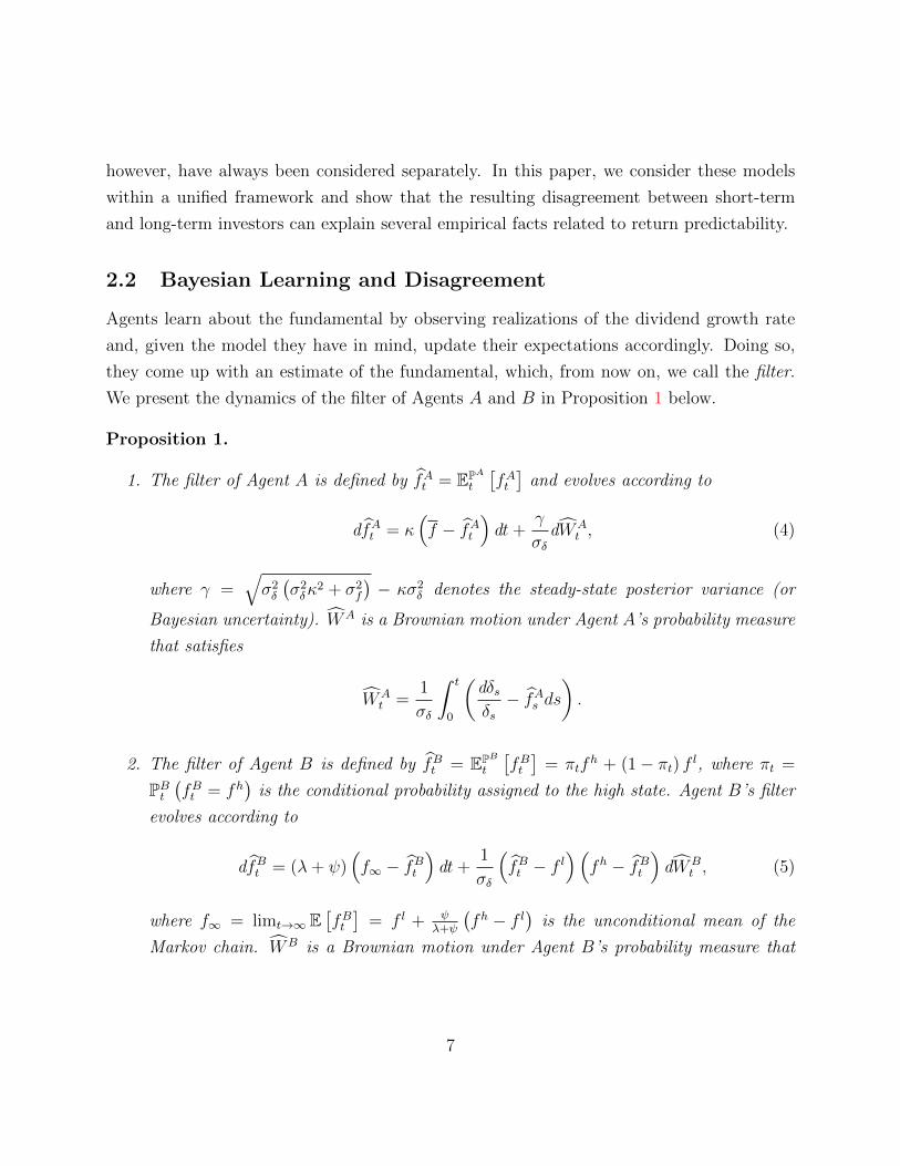
We present the dynamics of the filter of Agents A and B in Proposition 1 below.
Proposition 1. aaa
1. The filter of Agent A is defined by fAt = EPAt
[fAt]
and evolves according to
dfAt = κ(f − fAt
)dt+
γ
σδdWA
t , (4)
where γ =√σ2δ
(σ2δκ
2 + σ2f
)− κσ2
δ denotes the steady-state posterior variance (or
Bayesian uncertainty). WA is a Brownian motion under Agent A’s probability measure
that satisfies
WAt =
1
σδ
∫ t
0
(dδsδs− fAs ds
).
2. The filter of Agent B is defined by fBt = EPBt
[fBt]
= πtfh + (1− πt) f l, where πt =
PBt(fBt = fh
)is the conditional probability assigned to the high state. Agent B’s filter
evolves according to
dfBt = (λ+ ψ)(f∞ − fBt
)dt+
1
σδ
(fBt − f l
)(fh − fBt
)dWB
t , (5)
where f∞ = limt→∞ E[fBt]
= f l + ψλ+ψ
(fh − f l
)is the unconditional mean of the
Markov chain. WB is a Brownian motion under Agent B’s probability measure that
7
satisfies
WBt =
1
σδ
∫ t
0
(dδsδs− fBs ds
).
Proof. aaa
1. See Appendix A.1.
2. See Lipster and Shiryaev (2001).
Learning preserves the mean-reversion of Agent A’s initial model. Her views revert
towards their long-term mean f at speed κ, as shown in Eq. (4): when her filter is below
f her expectations revert upwards and when her filter is above f her expectations revert
downwards. In Section 3.1, we calibrate her model to the U.S. business cycle and find that
the estimated reversion speed is low. As a result, Agent A adjusts her views slowly. That
is, Agent A is a “slow learner”.
The mechanism through which Agent B updates her views differs from that of Agent A.
Her views also mean-revert, yet at a different speed λ + ψ 6= κ and to a different long-term
mean f∞ 6= f , as shown in Eq. (5). Unlike Agent A’s filter that mechanically inherits the
persistence of her initial model, the mean-reversion in Agent B’s filter reflects her effort to
continuously reassess the likelihood of the high state using the information that continuously
flows from dividends. Whether Agent B is faster to adjust her expectations than Agent A
not only depends on her relative mean-reversion speed, but also on the volatility of her filter.
Unlike the volatility of Agent A’s filter, which is constant, the volatility of Agent B’s filter
is stochastic and can therefore change precipitously. That is, Agent B is a “fast learner”.
Sudden changes in Agent B’s expectations typically occur when she is most uncertain
about the current state of the economy, i.e., when she assigns equal probabilities to each
state:
fm ≡1
2f l +
1
2fh.
As her expectations drop below fm, her filter is rapidly attracted towards the down state;
when her expectations rises above fm, her filter gets rapidly absorbed towards the up state.
8
In Section 3.1, we calibrate her model and find that the up state is more persistent than the
down state—the estimated intensity ψ is larger than λ. This asymmetry between the two
regimes implies that her filter tends to stick around the up state over a longer time period.
For reasons that will become apparent in Section 3.1, we choose to work under Agent
A’s probability measure. We convert Agent A’s views into those of Agent B through the
following change of measure:
dPB
dPA
∣∣∣∣Ft
≡ ηt = exp
[−1
2
∫ t
0
g2u
σ2δ
du−∫ t
0
guσδ
dWAu
], (6)
where the process g ≡ fA − fB represents agents’ disagreement about the estimated funda-
mental.
The change of measure in (6) implies that Agents A and B have equivalent perceptions
of the world.14 In particular, the Brownian motions WA and WB are related through
dWBt = dWA
t +gtσδ
dt.
That agents have equivalent perceptions may be surprising, if we consider that Agent B’s
filter is strictly confined within the interval [f l, fh], while Agent A’s filter can reach virtually
any value. To see how both views are compatible, fix a value for Agent A’s filter, say fA
.
This, in turn, imposes a restriction on the possible values of disagreement. Specifically, since
Agent B assigns zero probabilities to the events fB > fh and fB < f l, disagreement is
at least equal to fA − fh and at most equal to f
A − f l. The dynamics of disagreement, g,
are such that this property is always satisfied:
dgt =
[κ(f − fAt
)− (λ+ ψ)
(f∞ + gt − fAt
)− gtσ2δ
(fAt − gt − f l
)(fh + gt − fAt
)]dt
+γ −
(fAt − gt − f l
)(fh + gt − fAt
)σδ
dWAt . (7)
14Disagreement is the difference between an Ornstein-Uhlenbeck process, which is stationary, and abounded process. Disagreement is therefore stationary, the Novikov condition is satisfied and Girsanov’sTheorem applies.
9
The dynamics in Eq. (7) reflect our previous discussion regarding the different learning
mechanisms of the two agents. In particular, agents disagree about three aspects of the
fundamental: its persistence, its long-term mean, and its volatility. These three aspects
together give rise to countercyclical disagreement that persists over long horizons, consis-
tent with the observed pattern of disagreement among professional forecasters (Patton and
Timmermann (2010)). The key ingredient to generate this pattern of disagreement is that
agents use heterogeneous models,15 an assumption that also finds strong empirical support
(e.g., Kandel and Pearson (1995) and Patton and Timmermann (2010)). To consistently
measure disagreement in our model, we let agents calibrate their model to the U.S. business
cycle (Section 3.1) and postpone an extensive discussion of the resulting term structure of
disagreement to Section 3.2.
2.3 Equilibrium
Agents choose their portfolios and consumption plans to maximize their expected lifetime
utility of consumption. They have power utility preferences defined by
U (c, t) ≡ e−ρtc1−α
1− α,
where α > 0 is the coefficient of relative risk aversion and ρ > 0 the subjective discount rate.
Since markets are complete, we solve the consumption-portfolio problem of both agents
using the martingale approach of Karatzas, Lehoczky, and Shreve (1987) and Cox and Huang
(1989). Each agent’s maximization problem is described and solved in Appendix A.2. Im-
posing the market-clearing condition gives the state-price density ξ, which satisfies:
ξt = e−ρtδ−αt
[(ηtφB
) 1α
+
(1
φA
) 1α
]α, (8)
where φA and φB are the Lagrange multipliers associated to Agent A’s and Agent B’s budget
constraints, respectively.
The main mechanism generating stronger predictability in recessions operates through
15These dynamics are specific to model heterogeneity. When agents disagree about the parameters of asame model, the dynamics of disagreement differ significantly. See, for instance, David (2008), Buraschi andWhelan (2013), Ehling et al. (2013), Andrei et al. (2014), and Buraschi et al. (2014).
10
Eq. (8). Heterogeneous beliefs affect the state-price density through the variable η, the
likelihood of Agent B’s model relative to Agent A’s model. This relative likelihood is, in turn,
determined by the disagreement process (through Eq. (6)). As a result, the disagreement
process drives the dynamics of the state-price density and, hence, the dynamics of stock
returns. In particular, Dumas et al. (2009) note that ξ is concave in η; Jensen’s inequality
along with Eq. (6) together imply that an increase in disagreement reduces the expected
values of future state-price densities under Agent A’s measure, resulting in higher expected
returns. Because fluctuations in disagreement are faster and stronger in recessions (see
Section 3.2), disagreement better predicts future returns in recessions.
An application of Ito’s lemma to the state-price density in Eq. (8) yields the equilibrium
risk-free rate, rf , and market price of risk, θ, of our model:
rft = ρ+ αfAt −1
2α(α + 1)σ2
δ + (1− ω(ηt)) gt
(1
2
α− 1
ασ2δ
ω(ηt)gt − α)
(9)
θt = ασδ +(1− ω(ηt))
σδgt, (10)
where ω(η) denotes Agent A’s consumption share, which we define in Appendix A.2.
If agents did not disagree (g = 0) or if only one agent populated the economy (ω = 0
or ω = 1), the risk-free rate in Eq. (9) and the market price of risk in Eq. (10) would be
those of Lucas (1978). Inspecting the last term in Eq. (10), we conclude that heterogeneous
beliefs cause the market price of risk to exceed that of a Lucas (1978) economy, but only
when Agent A is more optimistic than Agent B (g > 0). In our model, this outcome, which
plays an important role when we study agents’ profits in Section 5, only arises in recessions.
Finally, we provide the equilibrium stock price in Proposition 2 below.
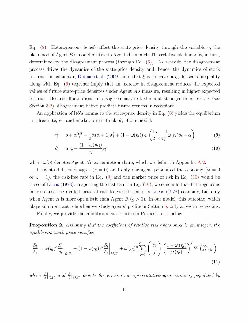
Proposition 2. Assuming that the coefficient of relative risk aversion α is an integer, the
equilibrium stock price satisfies
Stδt
= ω(ηt)αStδt
∣∣∣∣O.U.
+ (1− ω(ηt))αStδt
∣∣∣∣M.C.
+ ω (ηt)αα−1∑j=1
(α
j
)(1− ω (ηt)
ω (ηt)
)jF j(fAt , gt
)(11)
where Sδ
∣∣O.U.
and Sδ
∣∣M.C.
denote the prices in a representative-agent economy populated by
11
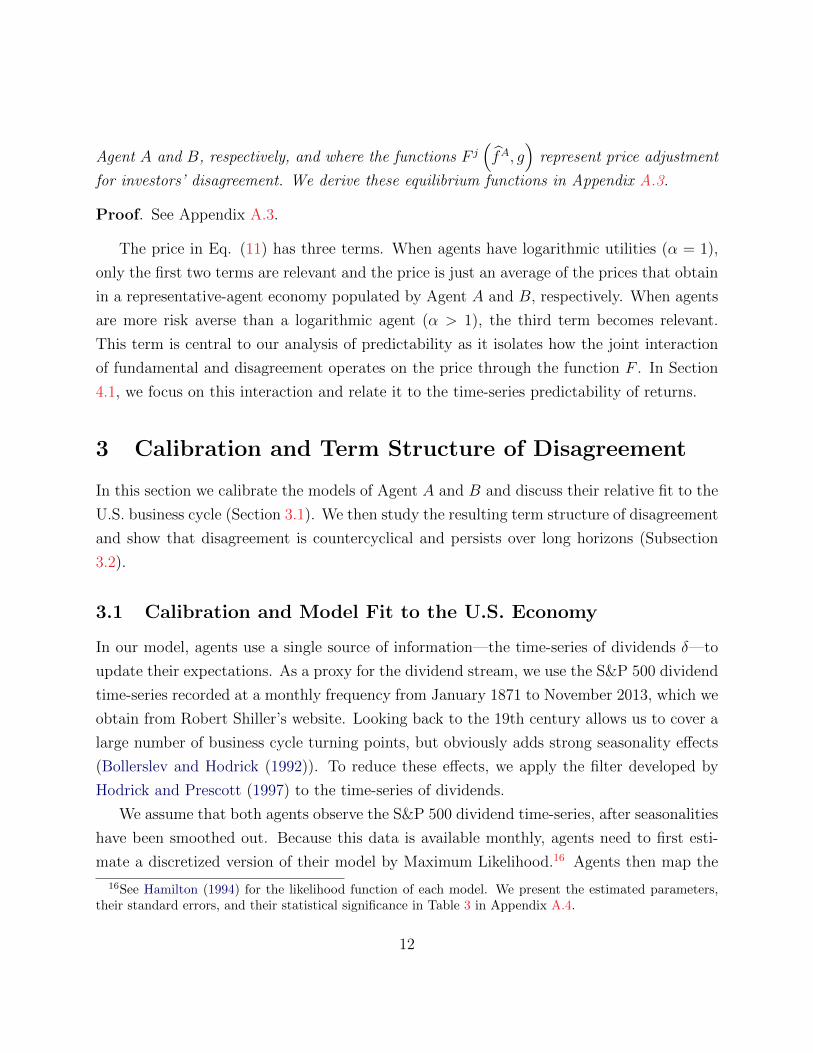
Agent A and B, respectively, and where the functions F j(fA, g
)represent price adjustment
for investors’ disagreement. We derive these equilibrium functions in Appendix A.3.
Proof. See Appendix A.3.
The price in Eq. (11) has three terms. When agents have logarithmic utilities (α = 1),
only the first two terms are relevant and the price is just an average of the prices that obtain
in a representative-agent economy populated by Agent A and B, respectively. When agents
are more risk averse than a logarithmic agent (α > 1), the third term becomes relevant.
This term is central to our analysis of predictability as it isolates how the joint interaction
of fundamental and disagreement operates on the price through the function F . In Section
4.1, we focus on this interaction and relate it to the time-series predictability of returns.
3 Calibration and Term Structure of Disagreement
In this section we calibrate the models of Agent A and B and discuss their relative fit to the
U.S. business cycle (Section 3.1). We then study the resulting term structure of disagreement
and show that disagreement is countercyclical and persists over long horizons (Subsection
3.2).
3.1 Calibration and Model Fit to the U.S. Economy
In our model, agents use a single source of information—the time-series of dividends δ—to
update their expectations. As a proxy for the dividend stream, we use the S&P 500 dividend
time-series recorded at a monthly frequency from January 1871 to November 2013, which we
obtain from Robert Shiller’s website. Looking back to the 19th century allows us to cover a
large number of business cycle turning points, but obviously adds strong seasonality effects
(Bollerslev and Hodrick (1992)). To reduce these effects, we apply the filter developed by
Hodrick and Prescott (1997) to the time-series of dividends.
We assume that both agents observe the S&P 500 dividend time-series, after seasonalities
have been smoothed out. Because this data is available monthly, agents need to first esti-
mate a discretized version of their model by Maximum Likelihood.16 Agents then map the
16See Hamilton (1994) for the likelihood function of each model. We present the estimated parameters,their standard errors, and their statistical significance in Table 3 in Appendix A.4.
12
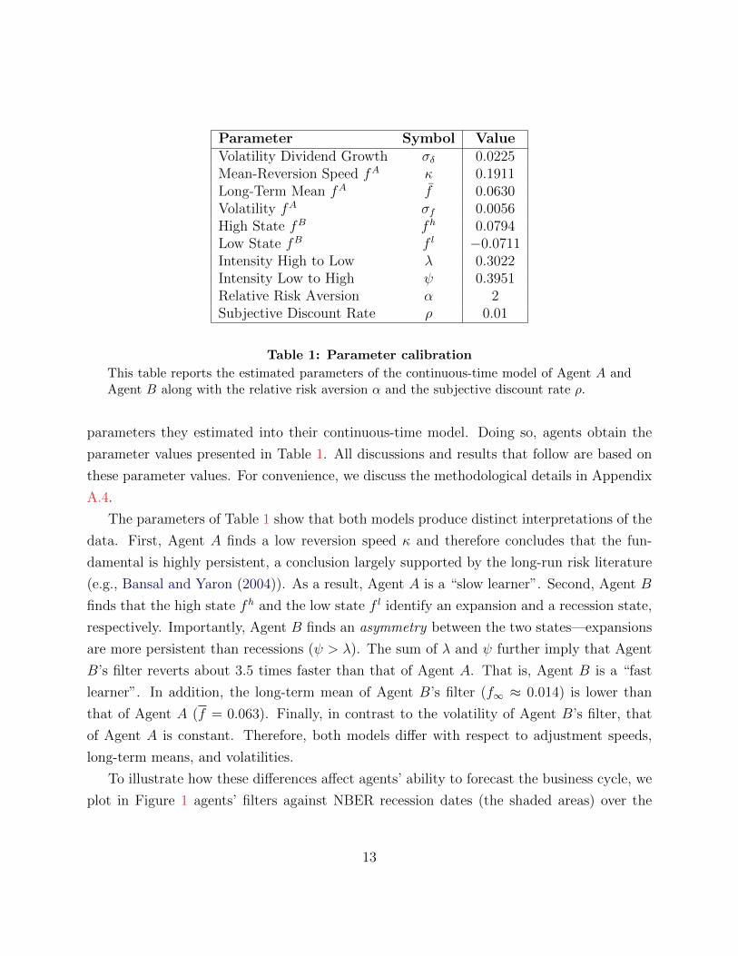
Parameter Symbol ValueVolatility Dividend Growth σδ 0.0225Mean-Reversion Speed fA κ 0.1911Long-Term Mean fA f 0.0630Volatility fA σf 0.0056High State fB fh 0.0794Low State fB f l −0.0711Intensity High to Low λ 0.3022Intensity Low to High ψ 0.3951Relative Risk Aversion α 2Subjective Discount Rate ρ 0.01
Table 1: Parameter calibration
This table reports the estimated parameters of the continuous-time model of Agent A andAgent B along with the relative risk aversion α and the subjective discount rate ρ.
parameters they estimated into their continuous-time model. Doing so, agents obtain the
parameter values presented in Table 1. All discussions and results that follow are based on
these parameter values. For convenience, we discuss the methodological details in Appendix
A.4.
The parameters of Table 1 show that both models produce distinct interpretations of the
data. First, Agent A finds a low reversion speed κ and therefore concludes that the fun-
damental is highly persistent, a conclusion largely supported by the long-run risk literature
(e.g., Bansal and Yaron (2004)). As a result, Agent A is a “slow learner”. Second, Agent B
finds that the high state fh and the low state f l identify an expansion and a recession state,
respectively. Importantly, Agent B finds an asymmetry between the two states—expansions
are more persistent than recessions (ψ > λ). The sum of λ and ψ further imply that Agent
B’s filter reverts about 3.5 times faster than that of Agent A. That is, Agent B is a “fast
learner”. In addition, the long-term mean of Agent B’s filter (f∞ ≈ 0.014) is lower than
that of Agent A (f = 0.063). Finally, in contrast to the volatility of Agent B’s filter, that
of Agent A is constant. Therefore, both models differ with respect to adjustment speeds,
long-term means, and volatilities.
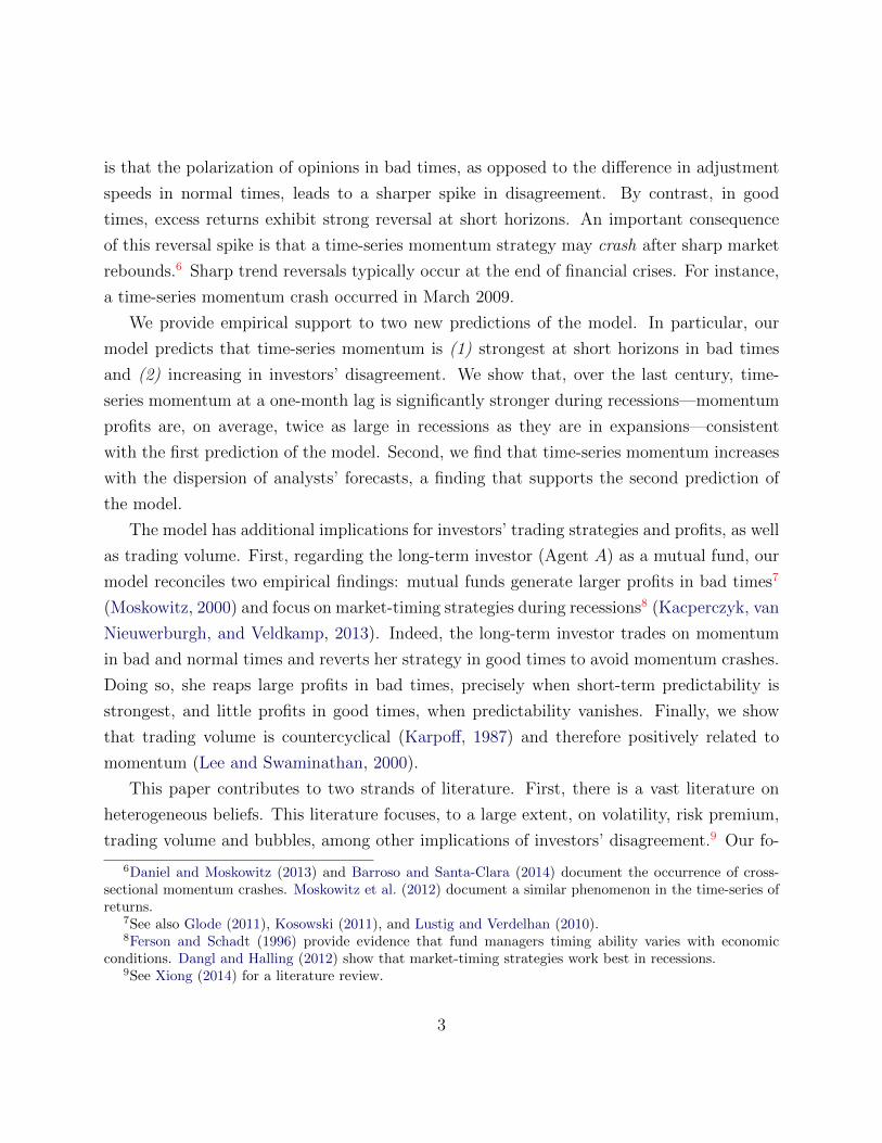
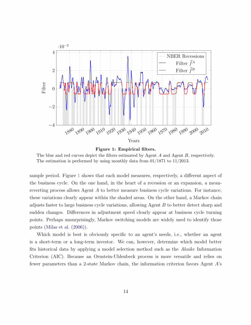
To illustrate how these differences affect agents’ ability to forecast the business cycle, we
plot in Figure 1 agents’ filters against NBER recession dates (the shaded areas) over the
13
18801890
19001910
19201930
19401950
19601970
19801990
20002010
−4
−2
0
2
4·10−2
Years
Filte
r
NBER Recessions
Filter fA
Filter fB
Figure 1: Empirical filters.
The blue and red curves depict the filters estimated by Agent A and Agent B, respectively.The estimation is performed by using monthly data from 01/1871 to 11/2013.
sample period. Figure 1 shows that each model measures, respectively, a different aspect of
the business cycle. On the one hand, in the heart of a recession or an expansion, a mean-
reverting process allows Agent A to better measure business cycle variations. For instance,
these variations clearly appear within the shaded areas. On the other hand, a Markov chain
adjusts faster to large business cycle variations, allowing Agent B to better detect sharp and
sudden changes. Differences in adjustment speed clearly appear at business cycle turning
points. Perhaps unsurprisingly, Markov switching models are widely used to identify those
points (Milas et al. (2006)).
Which model is best is obviously specific to an agent’s needs, i.e., whether an agent
is a short-term or a long-term investor. We can, however, determine which model better
fits historical data by applying a model selection method such as the Akaike Information
Criterion (AIC). Because an Ornstein-Uhlenbeck process is more versatile and relies on
fewer parameters than a 2-state Markov chain, the information criterion favors Agent A’s
14
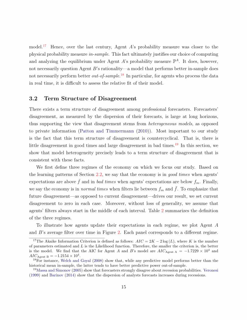
model.17 Hence, over the last century, Agent A’s probability measure was closer to the
physical probability measure in-sample. This fact ultimately justifies our choice of computing
and analyzing the equilibrium under Agent A’s probability measure PA. It does, however,
not necessarily question Agent B’s rationality—a model that performs better in-sample does
not necessarily perform better out-of-sample.18 In particular, for agents who process the data
in real time, it is difficult to assess the relative fit of their model.
3.2 Term Structure of Disagreement
There exists a term structure of disagreement among professional forecasters. Forecasters’
disagreement, as measured by the dispersion of their forecasts, is large at long horizons,
thus supporting the view that disagreement stems from heterogeneous models, as opposed
to private information (Patton and Timmermann (2010)). Most important to our study
is the fact that this term structure of disagreement is countercyclical. That is, there is
little disagreement in good times and large disagreement in bad times.19 In this section, we
show that model heterogeneity precisely leads to a term structure of disagreement that is
consistent with these facts.
We first define three regimes of the economy on which we focus our study. Based on
the learning patterns of Section 2.2, we say that the economy is in good times when agents’
expectations are above f and in bad times when agents’ expectations are below fm. Finally,
we say the economy is in normal times when filters lie between fm and f . To emphasize that
future disagreement—as opposed to current disagreement—drives our result, we set current
disagreement to zero in each case. Moreover, without loss of generality, we assume that
agents’ filters always start in the middle of each interval. Table 2 summarizes the definition
of the three regimes.
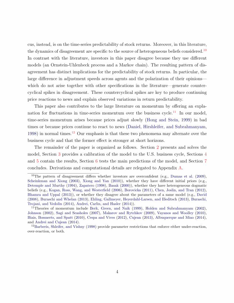
To illustrate how agents update their expectations in each regime, we plot Agent A
and B’s average filter over time in Figure 2. Each panel corresponds to a different regime.
17The Akaike Information Criterion is defined as follows: AIC = 2K − 2 log (L), where K is the numberof parameters estimated and L is the Likelihood function. Therefore, the smaller the criterion is, the betteris the model. We find that the AIC for Agent A and B’s model are AICAgent A = −1.7229 × 10⁴ andAICAgent B = −1.2154× 10⁴.
18For instance, Welch and Goyal (2008) show that, while any predictive model performs better than thehistorical mean in-sample, the latter tends to have better predictive power out-of-sample.
19Massa and Simonov (2005) show that forecasters strongly disagree about recession probabilities. Veronesi(1999) and Barinov (2014) show that the dispersion of analysts forecasts increases during recessions.
15
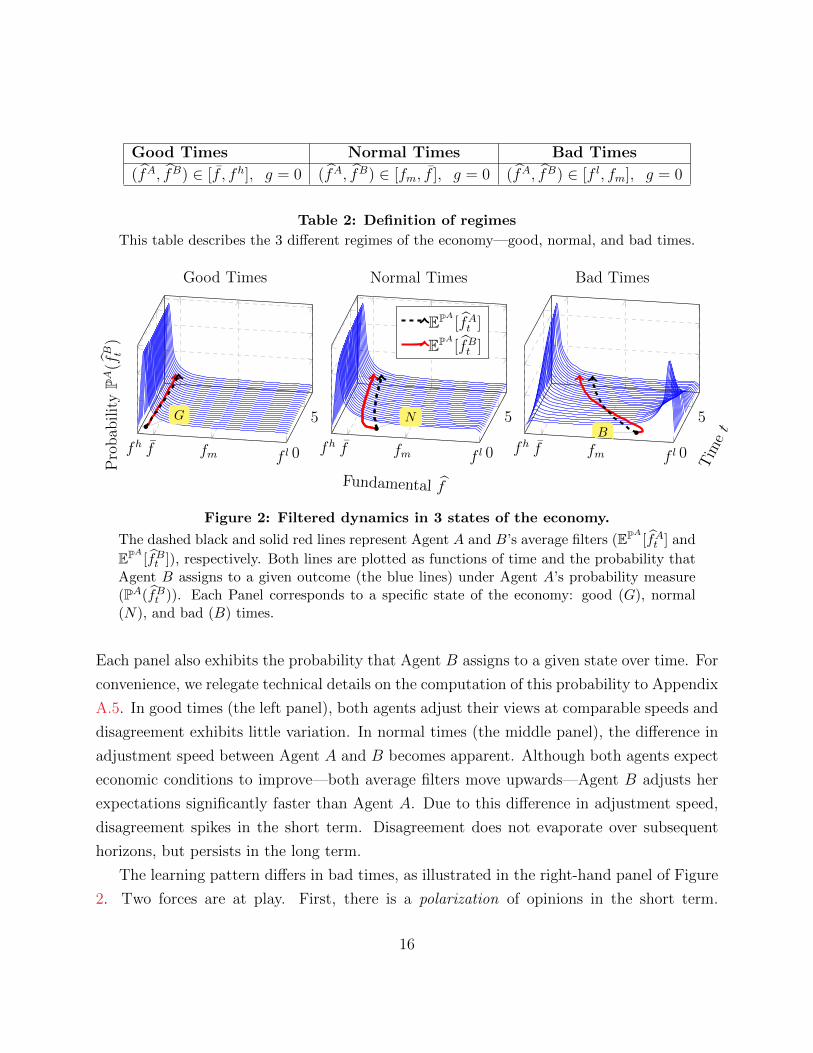
Good Times Normal Times Bad Times
(fA, fB) ∈ [f , fh], g = 0 (fA, fB) ∈ [fm, f ], g = 0 (fA, fB) ∈ [f l, fm], g = 0
Table 2: Definition of regimes
This table describes the 3 different regimes of the economy—good, normal, and bad times.
0
5
f lfmffh
G
Pro
bab
ilit
yPA
(fB t
)
Good Times
0
5
f lfmffh
N
Fundamental f
Normal Times
EPA [fAt ]
EPA [fBt ]
0
5
f lfmffhB
Tim
et
Bad Times
Figure 2: Filtered dynamics in 3 states of the economy.
The dashed black and solid red lines represent Agent A and B’s average filters (EPA [fAt ] and
EPA [fBt ]), respectively. Both lines are plotted as functions of time and the probability thatAgent B assigns to a given outcome (the blue lines) under Agent A’s probability measure(PA(fBt )). Each Panel corresponds to a specific state of the economy: good (G), normal(N), and bad (B) times.
Each panel also exhibits the probability that Agent B assigns to a given state over time. For
convenience, we relegate technical details on the computation of this probability to Appendix
A.5. In good times (the left panel), both agents adjust their views at comparable speeds and
disagreement exhibits little variation. In normal times (the middle panel), the difference in
adjustment speed between Agent A and B becomes apparent. Although both agents expect
economic conditions to improve—both average filters move upwards—Agent B adjusts her
expectations significantly faster than Agent A. Due to this difference in adjustment speed,
disagreement spikes in the short term. Disagreement does not evaporate over subsequent
horizons, but persists in the long term.
The learning pattern differs in bad times, as illustrated in the right-hand panel of Figure
2. Two forces are at play. First, there is a polarization of opinions in the short term.
16
That is, agents disagree about the direction in which the economy is heading and average
filters diverge. In particular, Agent A is optimistic and expects the economy to recover,
while Agent B is pessimistic and expects economic conditions to further deteriorate. This
polarization of opinions creates a spike in disagreement in the short term. Second, the
difference in adjustment speed reappears in the long run. As Agent B realizes that the
economy is recovering, she rapidly catches up with Agent A and eventually becomes more
optimistic than Agent A. As a result, disagreement evaporates in the medium term and
regenerates in the long term through the difference in adjustment speeds (Agent B adjusts
her views significantly faster than Agent A).
Overall, the polarization of opinions in the short term along with the difference in adjust-
ment speeds in the long term generate strong disagreement in bad times. This conclusion is
consistent with empirical evidence. In particular, Veronesi (1999), Patton and Timmermann
(2010), Carlin et al. (2013), and Barinov (2014) find that disagreement is larger in downturns
than in upturns.
4 Disagreement driving Stock Return Predictability
Recent evidence shows that stock return predictability is concentrated in bad times.20 In
this section, our objective is to determine the mechanism that causes return predictability to
vary over the business cycle. We show that countercyclical disagreement leads to downward
price pressures (Section 4.1) and continuing price reaction to past news (Section 4.2), which
are concentrated in bad times. Moreover, we show that these phenomena produce time-series
momentum and crashes in time-series momentum following sharp market rebounds (Section
4.3).
4.1 Disagreement and Downward Price Pressure
There is evidence that high disagreement predicts low future returns at short horizons (e.g.,
Diether et al. (2002)). Recently, Cen et al. (2014) find that this relation is concentrated in
bad times. In this section, we show that our model offers an explanation for this fact.
20Garcia (2013) shows that the content of news better predict stock returns in recessions. Rapach, Strauss,and Zhou (2010), Henkel, Martin, and Nardari (2011), and Dangl and Halling (2012) find that macro variableshave better predictive power in recessions.
17
In our model, predictability arises through the relation between disagreement and fun-
damentals. This relation operates on prices through two opposite forces. On the one hand,
an increase in the fundamental and/or in relative optimism improves investment opportuni-
ties. As a result, agents delay consumption to increase their holdings in the stock and the
price increases. We call this the investment effect. On the other hand, an increase in the
fundamental and/or in relative optimism predicts high future consumption. Because agents
want to smooth consumption over time, they disinvest to consume more today and the price
decreases. We call this the consumption effect.
Whether the investment or the consumption effect dominates depends on the interac-
tion between fundamental and disagreement in the future and therefore on the state of the
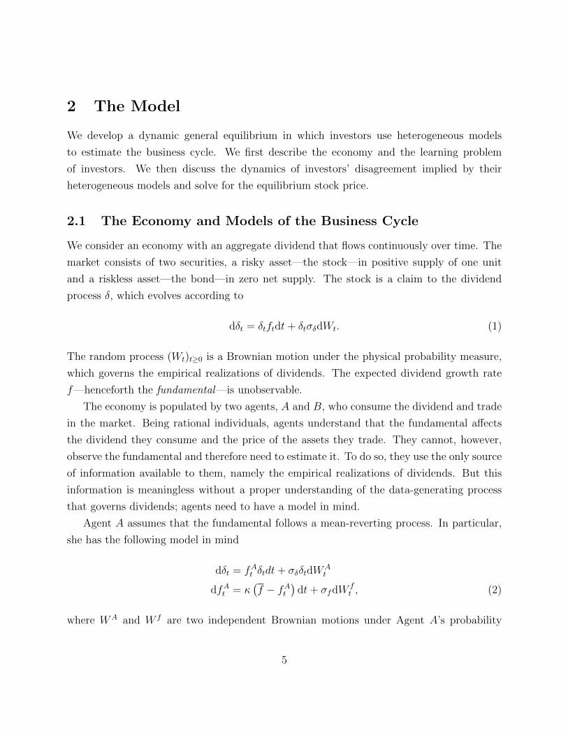
economy. To show this, we first isolate the component of prices that exclusively captures
this interaction, namely the function F in Eq. (11). We plot this price component (the
blue surface) in Figure 3, both as a function of disagreement and fundamental. This sur-
face provides a static view on prices, disagreement, and fundamental. To understand how
these three dimensions interact dynamically, we draw their average path over time (the red
arrows). In general, the higher the fundamental is, the stronger the investment effect is. We
now study in which regime the investment effect actually dominates.
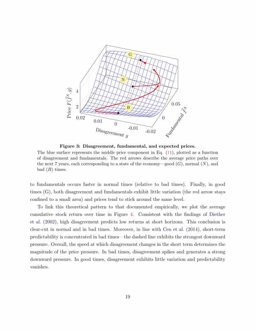
In bad times (B), polarization of opinions creates a spike in disagreement in the short
term, causing Agent A to be optimistic relative to Agent B (the red arrow moves towards
the left). This spike in disagreement dominates reversion to fundamentals in the short-term
(the red arrow does not revert upwards immediately). In this case, the consumption effect
is stronger and disagreement therefore causes a strong downward pressure on prices. As
Agent B realizes the economy is recovering, opinions align and agent’s expectations only
differ with respect to their adjustment speed (the red arrow changes direction). A decrease
in disagreement in turn allows reversion to fundamentals to drive prices back up. Hence, in
the long term, the investment effect dominates.
In normal times (N), difference in adjustment speeds produces a spike in disagreement
in the short term, causing Agent A to be pessimistic relative to Agent B (the red arrow
moves towards the right). As in bad times, disagreement dominates reversion to fundamen-
tals in the short term, which leads to a downward price pressure. In this case, however, the
downward price pressure arises through the investment effect. Moreover, because disagree-
ment decreases monotonically over time (the red arrow reverts back towards zero), reversion
18
0
0.05
-0.02-0.01
00.01
0.02
2
4
N
G
B
Fund
amen
tal f
A
Disagreement g
Pri
ceF
(fA,g
)
Figure 3: Disagreement, fundamental, and expected prices.
The blue surface represents the middle price component in Eq. (11), plotted as a functionof disagreement and fundamentals. The red arrows describe the average price paths overthe next 7 years, each corresponding to a state of the economy—good (G), normal (N), andbad (B) times.
to fundamentals occurs faster in normal times (relative to bad times). Finally, in good
times (G), both disagreement and fundamentals exhibit little variation (the red arrow stays
confined to a small area) and prices tend to stick around the same level.
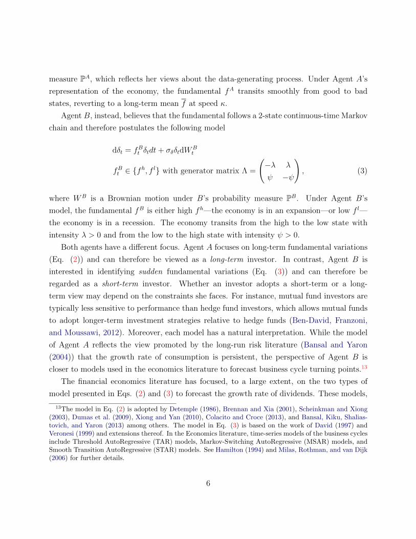
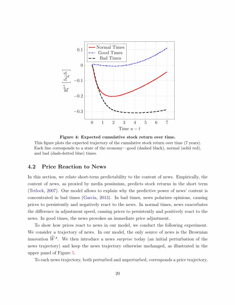
To link this theoretical pattern to that documented empirically, we plot the average
cumulative stock return over time in Figure 4. Consistent with the findings of Diether
et al. (2002), high disagreement predicts low returns at short horizons. This conclusion is
clear-cut in normal and in bad times. Moreover, in line with Cen et al. (2014), short-term
predictability is concentrated in bad times—the dashed line exhibits the strongest downward
pressure. Overall, the speed at which disagreement changes in the short term determines the
magnitude of the price pressure. In bad times, disagreement spikes and generates a strong
downward pressure. In good times, disagreement exhibits little variation and predictability
vanishes.
19
0 1 2 3 4 5 6 7
−0.3
−0.2
−0.1
0
0.1
Time u− t
EPA
t
[ S u−St
St
]Normal TimesGood TimesBad Times
Figure 4: Expected cumulative stock return over time.
This figure plots the expected trajectory of the cumulative stock return over time (7 years).Each line corresponds to a state of the economy—good (dashed black), normal (solid red),and bad (dash-dotted blue) times.
4.2 Price Reaction to News
In this section, we relate short-term predictability to the content of news. Empirically, the
content of news, as proxied by media pessimism, predicts stock returns in the short term
(Tetlock, 2007). Our model allows to explain why the predictive power of news’ content is
concentrated in bad times (Garcia, 2013). In bad times, news polarizes opinions, causing
prices to persistently and negatively react to the news. In normal times, news exacerbates
the difference in adjustment speed, causing prices to persistently and positively react to the
news. In good times, the news provokes an immediate price adjustment.
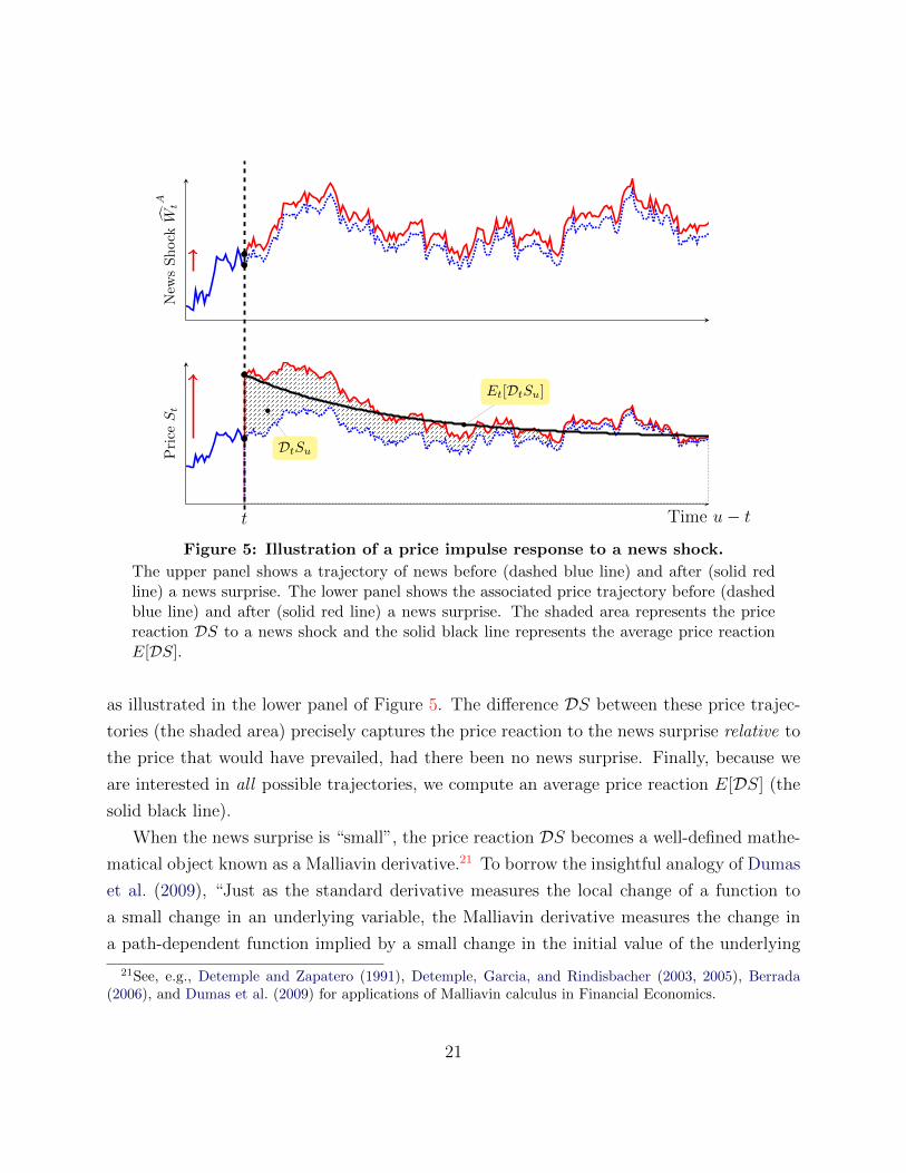
To show how prices react to news in our model, we conduct the following experiment.
We consider a trajectory of news. In our model, the only source of news is the Brownian
innovation WA. We then introduce a news surprise today (an initial perturbation of the
news trajectory) and keep the news trajectory otherwise unchanged, as illustrated in the
upper panel of Figure 5.
To each news trajectory, both perturbed and unperturbed, corresponds a price trajectory,
20
New
sS
hockW
t
A
t
Et[DtSu]
DtSu
Time u− t
Pri
ceSt
Figure 5: Illustration of a price impulse response to a news shock.
The upper panel shows a trajectory of news before (dashed blue line) and after (solid redline) a news surprise. The lower panel shows the associated price trajectory before (dashedblue line) and after (solid red line) a news surprise. The shaded area represents the pricereaction DS to a news shock and the solid black line represents the average price reactionE[DS].
as illustrated in the lower panel of Figure 5. The difference DS between these price trajec-
tories (the shaded area) precisely captures the price reaction to the news surprise relative to
the price that would have prevailed, had there been no news surprise. Finally, because we
are interested in all possible trajectories, we compute an average price reaction E[DS] (the
solid black line).
When the news surprise is “small”, the price reaction DS becomes a well-defined mathe-
matical object known as a Malliavin derivative.21 To borrow the insightful analogy of Dumas
et al. (2009), “Just as the standard derivative measures the local change of a function to
a small change in an underlying variable, the Malliavin derivative measures the change in
a path-dependent function implied by a small change in the initial value of the underlying
21See, e.g., Detemple and Zapatero (1991), Detemple, Garcia, and Rindisbacher (2003, 2005), Berrada(2006), and Dumas et al. (2009) for applications of Malliavin calculus in Financial Economics.
21
Brownian motions.” Its economic meaning is that of an impulse-response function following
a shock in initial values; in our case, a news shock. However, unlike a standard impulse-
response function, a Malliavin derivative takes future uncertainty into account. That is, it
does not assume that the world becomes deterministic after the shock has occurred. For
that reason, we compute an average price response, as described in Proposition 3.
Proposition 3. The expected average price response to a news surprise satisfies
EPAt [DtSu] = σδEPA
t [Su] +γ
κσδ
((1− αe−κ(u−t))EPA
t [Su] + (α− 1)EPAt
[∫ ∞u
ξsξuδse−κ(s−t)ds
])︸ ︷︷ ︸
fundamental effect
(12)
+1
σ2δ
EPAt
[∫ ∞u
ξsξuδs
((ω(ηs)− ω(ηu))
∫ u
t
gvDtgvdv − (1− ω(ηs))
∫ s
u
gvDtgvdv)
ds
]︸ ︷︷ ︸
disagreement effect
,
where the disagreement response Dg to a news surprise solves
dDtgv = ∇µg(fAv , gv)>(
γσδe−κ(v−t)
Dtgv
)dv +∇σg(fAv , gv)>
(γσδe−κ(v−t)
Dtgv
)dWA
v , (13)
with initial condition Dtgt = σg(fAt , gt) and where µg and σg represent the drift and the
diffusion of disagreement in Eq. (7), respectively. The operator ∇ stands for the gradient.
Proof. See Appendix A.6.
The news surprise affects prices through three different channels. The first term in Eq.
(12) represents the dividend channel; it is just a scaled average price, which we discussed
in the previous section. The second term captures the filter channel. This term is initially
negative; it becomes gradually positive and brings prices closer to their fundamental levels.
The last term accounts for the disagreement channel.
Our calibration indicates that the first two effects will be of small short-term magnitude as
compared to the disagreement channel. Disagreement is therefore the main channel through
which the price reacts to the news surprise in the short term. In particular, the news
22
0 1 2 3
−4
−2
0
2
4
Time u− t
EPA
t[D
tSu]
Price Impulse Responseaa
Normal TimesGood TimesBad Times
0 1 2 3
−1
0
1
·10−3
Bis
pes
sim
isti
cB
isov
erly
opti
mis
tic
Time u− t
EPA
t[guDtgu]
Disagreement Impulse Responseaa
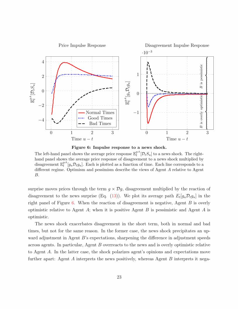
Figure 6: Impulse response to a news shock.
The left-hand panel shows the average price response EPAt [DtSu] to a news shock. The right-
hand panel shows the average price response of disagreement to a news shock multiplied bydisagreement EPA
t [guDtgu]. Each is plotted as a function of time. Each line corresponds to adifferent regime. Optimism and pessimism describe the views of Agent A relative to AgentB.
surprise moves prices through the term g × Dg, disagreement multiplied by the reaction of
disagreement to the news surprise (Eq. (13)). We plot its average path Et[guDtgu] in the
right panel of Figure 6. When the reaction of disagreement is negative, Agent B is overly
optimistic relative to Agent A; when it is positive Agent B is pessimistic and Agent A is
optimistic.
The news shock exacerbates disagreement in the short term, both in normal and bad
times, but not for the same reason. In the former case, the news shock precipitates an up-
ward adjustment in Agent B’s expectations, sharpening the difference in adjustment speeds
across agents. In particular, Agent B overreacts to the news and is overly optimistic relative
to Agent A. In the latter case, the shock polarizes agent’s opinions and expectations move
further apart: Agent A interprets the news positively, whereas Agent B interprets it nega-
23
tively. In good times, the reaction of disagreement is similar to that in normal times; it is,
however, less pronounced and less persistent.
We now study how the reaction of disagreement drives the reaction of prices. We plot
the 3-year average price response to a news shock today in the left panel of Figure 6. As
the news surprise hits, the price experiences an initial drop. In bad times (the black dashed
line), agents interpret the news in opposite ways and their dispute slows down the price
adjustment to the news shock. Because Agent B is pessimistic, the price continues to react
negatively to the news. The price then slowly corrects as opinions gradually align. In normal
times (the solid red line), while agents interpret the news shock in similar ways, Agent B
overreacts. Because Agent B is overly optimistic relative to Agent A, the price continues
to react positively to the news. The price then slowly corrects as Agent A catches up with
Agent B. In good times (the dash-dotted blue line), the news induces little disagreement
and prices revert immediately. Hence, the content of news predicts future returns (Tetlock,
2007) and this effect concentrates in bad times (Garcia, 2013).
Overall, in our model, prices continue to react to news only if disagreement spikes in
the short term. The polarization of opinions and the difference in adjustment speeds then
drive the direction of the price reaction. In bad times, Agent B’s pessimism slows down the
price reaction to the shock (decreasing reaction). In normal times, Agent B’s overreaction
accelerates the price response to the shock (increasing reaction). The former result resembles
the continuing under-reaction of Hong and Stein (1999), while the latter result is similar to
the continuing over-reaction of Daniel et al. (1998). Our emphasis is that these two effects
may alternate over the business cycle.
We now turn to the implications of these price reaction patterns for the serial correlation
of returns.
4.3 Implications for Time-Series Momentum and Momentum Crashes
One of the most pervasive facts in finance is momentum (Jegadeesh and Titman, 1993).
Recently, Moskowitz et al. (2012) uncover a similar pattern in the time-series of returns,
which they coin “time-series momentum”. Time-series momentum is a direct implication of
our previous results. In this section, we show that countercyclical disagreement can explain
both the term structure of time-series momentum and crashes in time-series momentum
24
0 10 20 30-0.12-0.1
-0.08-0.06-0.04-0.02
00.020.040.060.08
Ser
ial
Cor
rela
tion
ρt(h
)
Good Times
0 10 20 30
Lag h (Months)
Normal Times
0 10 20 30
Bad Times
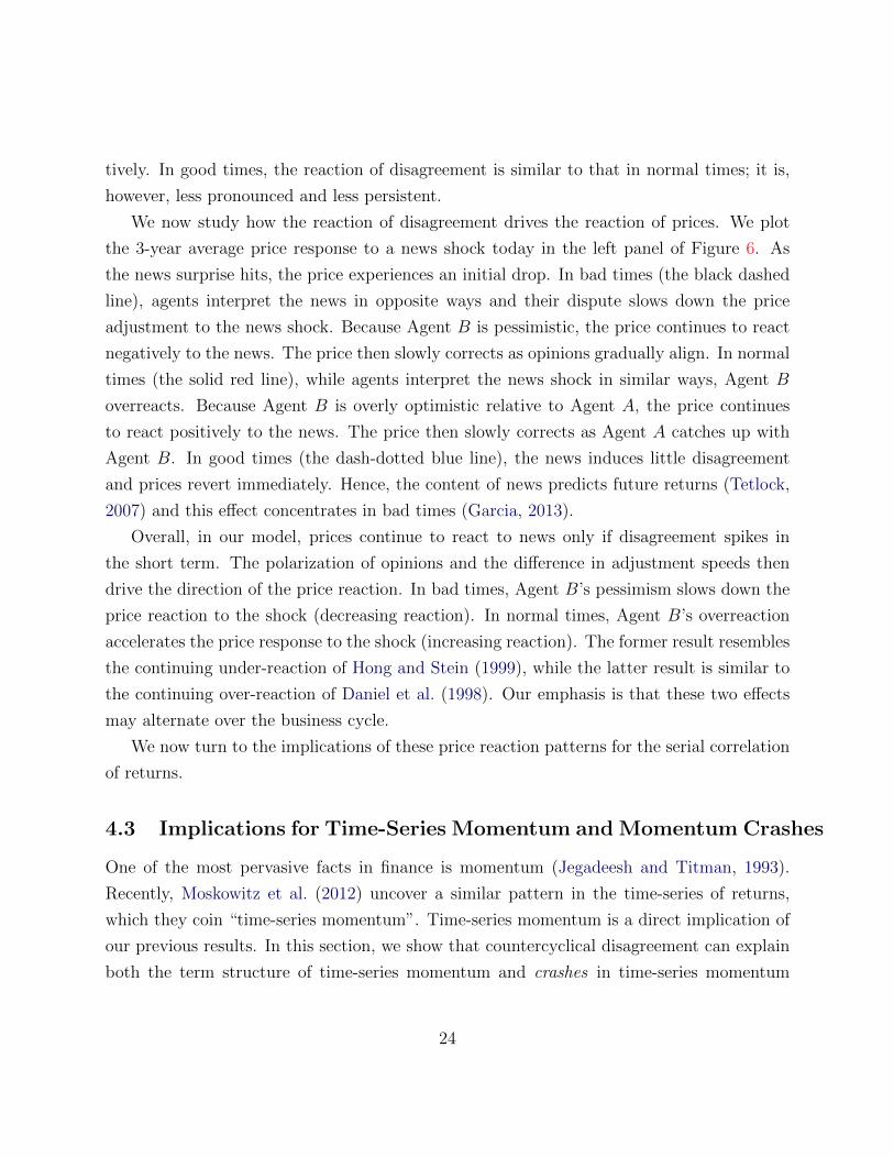
Figure 7: Serial correlation of excess returns.
This figure plots the serial correlation ρ(h) of excess returns for different lags h, rangingfrom 1 month to 3 years. Each panel corresponds to a different state of the economy.
following sharp market rebounds. Our model also predicts that time-series momentum is
strongest in bad times at a one-month lag, an implication that we test empirically (Section
6).
To study the implications of short-term predictability for the serial correlation of returns,
we focus on excess stock returns R, the dynamics of which satisfy
dRt =dSt + δtdt
St− rft dt = σt(θtdt+ dWA
t ).
We then compute the serial correlation of returns at different lags h according to
ρ(h) =covPA (Rt+h −Rt+h−1M , Rt −Rt−1M)
volPA
(Rt+h −Rt+h−1M) volPA
(Rt −Rt−1M),
where 1M stands for one month. The coefficient ρ(h) determines whether returns exhibit
momentum (ρ(h) > 0) or reversal (ρ(h) < 0). We plot this coefficient for different lags,
ranging from 1 month to 3 years, in Figure 7.
The serial correlation of returns has a similar term structure both in normal (the cen-
25

ter panel) and in bad times (the right panel). In particular, returns exhibit time-series
momentum over an horizon of 10 to 15 months, followed by reversal over subsequent hori-
zons. Moreover, the magnitude of momentum varies according to the horizon considered:
momentum is large at short horizons (up to three months) and then decays over longer
horizons. Both the magnitude and the time horizon of these effects are line with empirical
evidence. Moskowitz et al. (2012) find significant time-series momentum at short horizons
(1 to 6 months), weaker momentum at intermediate horizons (7 to 15 months), and reversal
at longer horizons. The pattern of serial correlation in our model is particularly consistent
with that documented for equity and commodities.
Based on our previous results, time-series momentum arises in our model because prices
continue to react to past news through the spike in disagreement. Hence, although similar,
the term structures of momentum in normal and in bad times differ in two respects. First,
because the price reaction to news shock is more persistent in normal times (see Figure
6), momentum persists over a longer horizon in that regime. Second, because the spike in
disagreement induced by the polarization of opinions is sharper than that induced by the
difference in adjustment speeds, momentum at a one-month lag is significantly larger in bad
times. This second implication finds strong empirical support (see Section 6).
Excess returns have different time-series properties in good times (the left panel). In
particular, returns exhibit strong reversal in the very short term and weak reversal over
subsequent months. The reason is that, in good times, the main force driving prices is
reversion to fundamentals, as opposed to disagreement (see Figure 6). Specifically, the
following mechanism operates. Suppose there is a bad news today. Investors, who want to
smooth consumption over time, save by increasing their holdings in the stock, thus causing
an immediate price increase. As the fundamental reverts, they unwind part of their stock
holdings, leading to a price decrease and thus to reversal.
An important consequence of the initial reversal spike in good times is that a time-series
momentum strategy may crash if the market rises sharply. To see this, suppose we start
implementing a momentum strategy in bad times. The right panel then indicates that this
strategy remains profitable as long as the market does not rise suddenly, i.e., as long as the
economy does not transit suddenly from bad to good times. If, instead, the market sharply
rebounds, the trend suddenly reverts and the momentum strategy crashes. Sharp trend
reversals typically occur at the end of financial crises. For instance, a time-series momentum
26
crash occurred at the end of the Global Financial Crisis in March, April and May of 2009
(Moskowitz et al., 2012). Daniel and Moskowitz (2013) and Barroso and Santa-Clara (2014)
document a similar phenomenon in the cross-section of stocks.
5 Trading Strategies and Momentum Timing
Evidence suggests that institutional investors exploit variations in return predictability to
time the market.22 In this section, our objective is to identify the trading strategy that
allows an investor to take advantage of short-term predictability over the business cycle. We
focus on the strategy of the long-term investor, Agent A. We show that she implements
a momentum strategy in bad and normal times and follows a contrarian strategy in good
times. Because predictability increases as economic conditions deteriorate, her strategy
makes significantly more money in bad times. In addition, we show that trading volume
is countercyclical and positively related to short-term momentum (Lee and Swaminathan
(2000)).
To identify Agent A’s trading strategy, we compute her wealth and deduce from it the
two components of her strategy. We highlight Agent A’s wealth in Proposition 4 below.
Proposition 4. Agent A’s wealth, V , satisfies
Vt = EPAt
[∫ ∞t
ξuξtcAudu
]= δtω (ηt)
αα−1∑j=0
(α− 1
j
)(1− ω (ηt)
ω (ηt)
)jEPAt
[∫ ∞t
e−ρ(u−t)(ηuηt
) jα(δuδt
)1−α
du
](α=2)
= δtω (ηt)2 Stδt
∣∣∣∣O.U.
+ δtω (ηt) (1− ω (ηt))F(fAt , gt
). (14)
Proof. See Dumas et al. (2009).
22Moskowitz (2000), Glode (2011), and Kosowski (2011) show that fund managers perform significantlybetter in recessions than in expansions. Kacperczyk et al. (2013) provide evidence that fund managers timethe market in recessions and pick stocks in expansions.
27
Our calibration (α = 2) implies that Agent A’s wealth is the sum of two terms, both
of which have an intuitive interpretation. If Agent A were the only agent populating the
economy, she would hold one unit of the stock over time, otherwise markets would not
clear. For that reason, her wealth would be exactly equal to the price that prevails in a
representative agent economy, hence the first term in Eq. (14). But, because she can trade
with Agent B, her portfolio fluctuates over time; it fluctuates in a way that reflects both her
expectations of the fundamental and how they differ from Agent B’s. The second term in
Eq. (14) precisely accounts for that. In particular, the function F is the price component
we plotted in Figure 3, which represents how the interaction between fundamentals and
disagreement operates on prices.
From Agent A’s wealth, we now deduce the strategy she implements. We present her
strategy in Proposition 5.
Proposition 5. The number Q of shares held by Agent A satisfies
Q =1
σS
∂V∂δ
σδδ +∂V
∂fA
γ
σδ+∂V
∂g
γ −(fA − g − f l
)(fh + g − fA
)σδ
− ∂V
∂η
gη
σδ
, (15)
where σ denotes the diffusion of stock returns, which satisfies
σ = σδ +1
S
∂S
∂fA
γ
σδ+∂S
∂g
γ −(fA − g − f l
)(fh + g − fA
)σδ
− ∂S
∂η
gη
σδ
. (16)
The number of shares Q ≡ M + H can be further decomposed into a myopic portfolio M =µ−rfασ2
VS
and a hedging portfolio
H = Q−M =α− 1
ασtStEPAt
[∫ ∞t
ξsξtcAs
(Dtξsξs− Dtξt
ξt
)ds
]. (17)
Proof. See Appendix A.7.
Agent A’s portfolio in Equation (15) has two parts. The first part, M , is a myopic
demand through which Agent A seeks to extract the immediate Sharpe ratio. The second
term, H, is an hedging demand through which Agent A seeks to exploit return predictability.
28
0 0.5 1 1.5 2 2.5 3
−1
−0.5
0
0.5
1
Contrariantrading
Momentumtrading
Time
Cor
r(dH,dP
)
Bad TimesNormal TimesGood Times
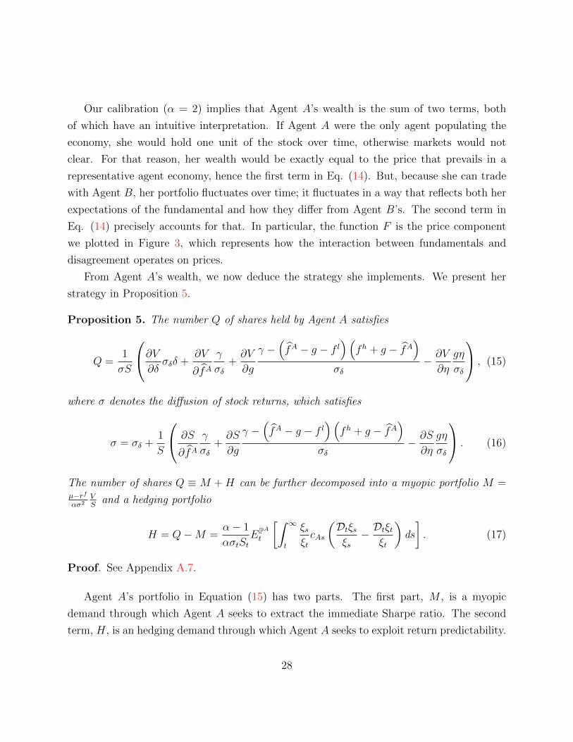
Figure 8: Model-implied trading behavior.
The solid red line, the dash-dotted blue line, and the dashed black line depict the averagecorrelation between the hedging component dH and the stock price dS in normal, good,and bad times, respectively. The correlation reported above is an average computed over100,000 simulations.
In particular, the term Dtξs in Eq. (17) indicates that Agent A performs the experiment of
Section 4.2. That is, she attempts to forecast how a news shock today affects future returns.
Because the hedging demand tells us how Agent A trades on return predictability, we focus
the analysis on this term.
5.1 Trading Strategies and Profits
To demonstrate how Agent A exploits return predictability, we follow Wang (1993) and
Brennan and Cao (1996) and compute the correlation, Corrt(dHt, dPt), between changes in
Agent A’s hedging portfolio and changes in stock prices. This correlation measures Agent
A’s trading behavior. A positive correlation means that Agent A tends to buy after price
increases and sell after price decreases, i.e., she is a momentum trader. Instead, a negative
correlation means that she is a contrarian. We plot this trading measure in Figure 8.
Agent A is a successful market timer. In the short-term (over the first year), she imple-
29
ments a momentum strategy both in normal times (the solid red line) and in bad times (the
dashed black line). In particular, Agent A anticipates that prices will continue to react to
news shocks in normal and bad times. Continuing price reaction in turn generates time-series
momentum, which she extracts by implementing a momentum strategy. Moreover, Agent
A recognizes that time-series momentum reverts faster in bad times than in normal times.
Therefore, in bad times, she eventually reverts her strategy and becomes a contrarian. In
good times, Agent A exclusively engages in contrarian trading (the dash-dotted blue line).
She anticipates that reversion to fundamentals will be fast and strong, and consistently
reverts her strategy. Doing so, she avoids crashes in time-series momentum and exploits
reversal.
Agent B takes the other side of the market. In normal times, because Agent A—the long-
term investor—is a momentum trader, Agent B—the short-term investor—is a contrarian.
Our model therefore predicts that long-term investors tend to be momentum traders, while
short-term investors tend to be contrarians. This prediction is in line with Goetzmann
and Massa (2002), who show that infrequent traders follow momentum strategies, whereas
frequent traders are contrarians.
We now want to understand in which state of the business cycle Agent A’s strategy is
most profitable. To do so, we compute the mean cumulative profit P that her strategy
generates. It satisfies
Pt =
∫ t
0
(QuSu −
µu − rfuασ2
u
Vu
)(µu − rfu
)du =
∫ t
0
HuSu(µu − rfu
)du. (18)
The profits in Eq. (18) represents the cumulative expected dollar amount made by following
a fully leveraged dynamic strategy that consists in borrowing HS dollars in the bond and
investing this amount in the stock. We plot the average cumulative profit P in Figure 9.
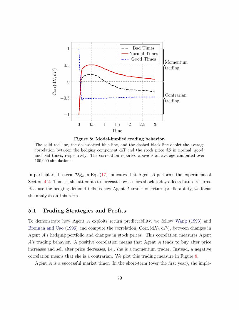
The profits that Agent A’s strategy generates are smallest in good times and largest in
bad times. The reason is as follows. In good times, prices accommodate news shocks almost
instantly, which makes it challenging for Agent A to reap large profits. In normal and bad
times, however, stock prices exhibit short-term predictability (continuing price reaction).
Agent A exploits this information to make larger profits. In particular, Agent A makes the
largest profits in bad times, that is when short-term predictability is strongest. Time-series
momentum therefore delivers larger profits in bad times (Moskowitz et al., 2012). Moreover,
30
0 0.5 1 1.5 2 2.5 3
0
1
2
3
Time
Pro
fit
Bad TimesNormal TimesGood Times
Figure 9: Model-implied trading profits.
The solid red line, the dash-dotted blue line, and the dashed black line depict the averageof the mean cumulative profit made by Agent A’s hedging strategy in normal, good, andbad times, respectively. The profit reported above is an average computed over 100,000simulations.
regarding Agent A, the long-term investor, as a mutual fund, our model reconciles two
empirical findings: mutual funds i) generate larger profits in bad times23 (Moskowitz (2000))
and ii) focus on market-timing strategies during recessions24 (Kacperczyk et al. (2013)).
5.2 Trading Volume
There is evidence that high disagreement (Verardo (2009)) and high trading volume (Lee
and Swaminathan (2000)) predict higher cross-sectional momentum. In this section, we
investigate how trading volume, disagreement, and time-series momentum are related. To
do so, we measure monthly trading volume by computing monthly absolute changes in the
23See also Glode (2011), Kosowski (2011), and Lustig and Verdelhan (2010).24Ferson and Schadt (1996) provide evidence that fund managers timing ability varies with economic
conditions. Dangl and Halling (2012) show that market-timing strategies work best in recessions.
31
diffusion of Agent A’s wealth:
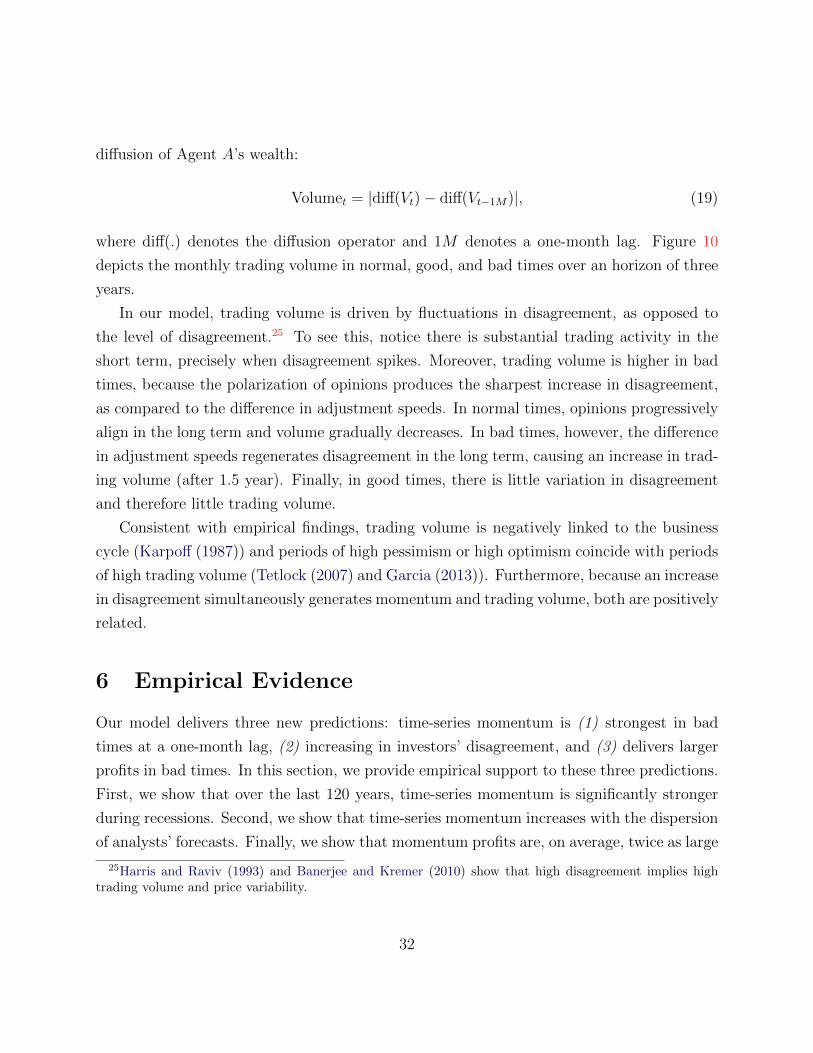
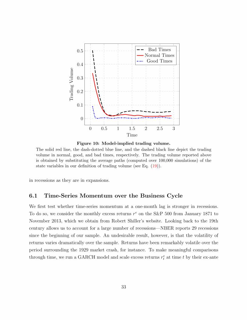
Volumet = |diff(Vt)− diff(Vt−1M)|, (19)
where diff(.) denotes the diffusion operator and 1M denotes a one-month lag. Figure 10
depicts the monthly trading volume in normal, good, and bad times over an horizon of three
years.
In our model, trading volume is driven by fluctuations in disagreement, as opposed to
the level of disagreement.25 To see this, notice there is substantial trading activity in the
short term, precisely when disagreement spikes. Moreover, trading volume is higher in bad
times, because the polarization of opinions produces the sharpest increase in disagreement,
as compared to the difference in adjustment speeds. In normal times, opinions progressively
align in the long term and volume gradually decreases. In bad times, however, the difference
in adjustment speeds regenerates disagreement in the long term, causing an increase in trad-
ing volume (after 1.5 year). Finally, in good times, there is little variation in disagreement
and therefore little trading volume.
Consistent with empirical findings, trading volume is negatively linked to the business
cycle (Karpoff (1987)) and periods of high pessimism or high optimism coincide with periods
of high trading volume (Tetlock (2007) and Garcia (2013)). Furthermore, because an increase
in disagreement simultaneously generates momentum and trading volume, both are positively
related.
6 Empirical Evidence
Our model delivers three new predictions: time-series momentum is (1) strongest in bad
times at a one-month lag, (2) increasing in investors’ disagreement, and (3) delivers larger
profits in bad times. In this section, we provide empirical support to these three predictions.
First, we show that over the last 120 years, time-series momentum is significantly stronger
during recessions. Second, we show that time-series momentum increases with the dispersion
of analysts’ forecasts. Finally, we show that momentum profits are, on average, twice as large
25Harris and Raviv (1993) and Banerjee and Kremer (2010) show that high disagreement implies hightrading volume and price variability.
32
0 0.5 1 1.5 2 2.5 3
0
0.1
0.2
0.3
0.4
0.5
Time
Tra
din
gV
olum
e
Bad TimesNormal TimesGood Times
Figure 10: Model-implied trading volume.
The solid red line, the dash-dotted blue line, and the dashed black line depict the tradingvolume in normal, good, and bad times, respectively. The trading volume reported aboveis obtained by substituting the average paths (computed over 100,000 simulations) of thestate variables in our definition of trading volume (see Eq. (19)).
in recessions as they are in expansions.
6.1 Time-Series Momentum over the Business Cycle
We first test whether time-series momentum at a one-month lag is stronger in recessions.
To do so, we consider the monthly excess returns re on the S&P 500 from January 1871 to
November 2013, which we obtain from Robert Shiller’s website. Looking back to the 19th
century allows us to account for a large number of recessions—NBER reports 29 recessions
since the beginning of our sample. An undesirable result, however, is that the volatility of
returns varies dramatically over the sample. Returns have been remarkably volatile over the
period surrounding the 1929 market crash, for instance. To make meaningful comparisons
through time, we run a GARCH model and scale excess returns ret at time t by their ex-ante
33
0 3 6 9 12−1
0
1
2
3
Lag h (Months)
β2,h
t-st
at
Excess Momentum: G(.) = sign(.)
0 3 6 9 12−1
0
1
2
3
Lag h (Months)β
2,h
t-st
at
Excess Momentum: G(.) = identity(.)
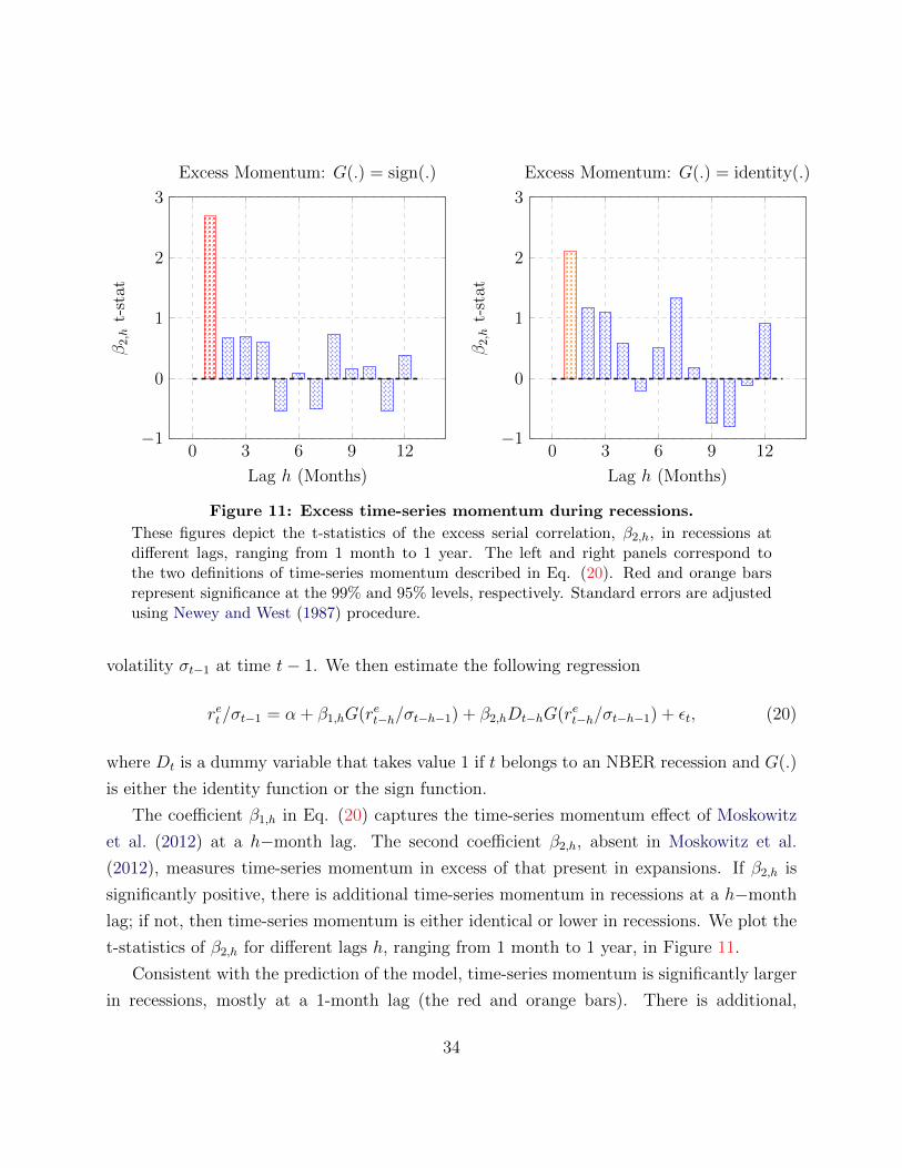
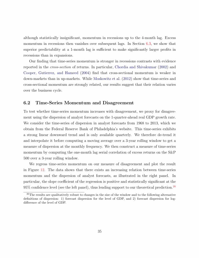
Figure 11: Excess time-series momentum during recessions.
These figures depict the t-statistics of the excess serial correlation, β2,h, in recessions atdifferent lags, ranging from 1 month to 1 year. The left and right panels correspond tothe two definitions of time-series momentum described in Eq. (20). Red and orange barsrepresent significance at the 99% and 95% levels, respectively. Standard errors are adjustedusing Newey and West (1987) procedure.
volatility σt−1 at time t− 1. We then estimate the following regression
ret/σt−1 = α + β1,hG(ret−h/σt−h−1) + β2,hDt−hG(ret−h/σt−h−1) + εt, (20)
where Dt is a dummy variable that takes value 1 if t belongs to an NBER recession and G(.)
is either the identity function or the sign function.
The coefficient β1,h in Eq. (20) captures the time-series momentum effect of Moskowitz
et al. (2012) at a h−month lag. The second coefficient β2,h, absent in Moskowitz et al.
(2012), measures time-series momentum in excess of that present in expansions. If β2,h is
significantly positive, there is additional time-series momentum in recessions at a h−month
lag; if not, then time-series momentum is either identical or lower in recessions. We plot the
t-statistics of β2,h for different lags h, ranging from 1 month to 1 year, in Figure 11.
Consistent with the prediction of the model, time-series momentum is significantly larger
in recessions, mostly at a 1-month lag (the red and orange bars). There is additional,
34
although statistically insignificant, momentum in recessions up to the 4-month lag. Excess
momentum in recessions then vanishes over subsequent lags. In Section 6.3, we show that
superior predictability at a 1-month lag is sufficient to make significantly larger profits in
recessions than in expansions.
Our finding that time-series momentum is stronger in recessions contrasts with evidence
reported in the cross-section of returns. In particular, Chordia and Shivakumar (2002) and
Cooper, Gutierrez, and Hameed (2004) find that cross-sectional momentum is weaker in
down-markets than in up-markets. While Moskowitz et al. (2012) show that time-series and
cross-sectional momentum are strongly related, our results suggest that their relation varies
over the business cycle.
6.2 Time-Series Momentum and Disagreement
To test whether time-series momentum increases with disagreement, we proxy for disagree-
ment using the dispersion of analyst forecasts on the 1-quarter-ahead real GDP growth rate.
We consider the time-series of dispersion in analyst forecasts from 1968 to 2013, which we
obtain from the Federal Reserve Bank of Philadelphia’s website. This time-series exhibits
a strong linear downward trend and is only available quarterly. We therefore de-trend it
and interpolate it before computing a moving average over a 3-year rolling window to get a
measure of dispersion at the monthly frequency. We then construct a measure of time-series
momentum by computing the one-month lag serial correlation of excess returns on the S&P
500 over a 3-year rolling window.
We regress time-series momentum on our measure of disagreement and plot the result
in Figure 12. The data shows that there exists an increasing relation between time-series
momentum and the dispersion of analyst forecasts, as illustrated in the right panel. In
particular, the slope coefficient of the regression is positive and statistically significant at the
95% confidence level (see the left panel), thus lending support to our theoretical prediction.26
26The results are qualitatively robust to changes in the size of the window and to the following alternativedefinitions of dispersion: 1) forecast dispersion for the level of GDP, and 2) forecast dispersion for log-difference of the level of GDP.
35
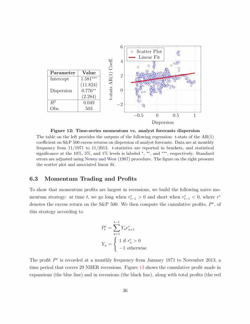
Parameter ValueIntercept 1.581∗∗∗
(11.824)Dispersion 0.776∗∗
(2.284)R2 0.049Obs. 503
−0.5 0 0.5 1
−2
0
2
4
6
Dispersion
t-st
ats
AR
(1)
Coeff
.
Scatter PlotLinear Fit
Figure 12: Time-series momentum vs. analyst forecasts dispersion
The table on the left provides the outputs of the following regression: t-stats of the AR(1)coefficient on S&P 500 excess returns on dispersion of analyst forecasts. Data are at monthlyfrequency from 11/1971 to 11/2013. t-statistics are reported in brackets, and statisticalsignificance at the 10%, 5%, and 1% levels is labeled ∗, ∗∗, and ∗∗∗, respectively. Standarderrors are adjusted using Newey and West (1987) procedure. The figure on the right presentsthe scatter plot and associated linear fit.
6.3 Momentum Trading and Profits
To show that momentum profits are largest in recessions, we build the following naive mo-
mentum strategy: at time t, we go long when ret−1 > 0 and short when ret−1 < 0, where re
denotes the excess return on the S&P 500. We then compute the cumulative profits, P e, of
this strategy according to
P et =
t−1∑u=1
Yureu+1
Yu =
1 if reu > 0
−1 otherwise
The profit P e is recorded at a monthly frequency from January 1871 to November 2013, a
time period that covers 29 NBER recessions. Figure 13 shows the cumulative profit made in
expansions (the blue line) and in recessions (the black line), along with total profits (the red
36
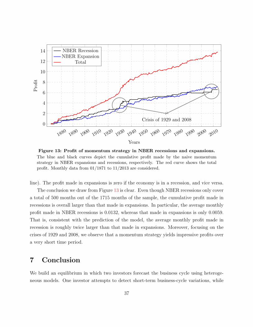
18801890
19001910
19201930
19401950
19601970
19801990
20002010
0
2
4
6
8
10
12
14
Crisis of 1929 and 2008
Years
Pro
fit
NBER RecessionNBER Expansion
Total
Figure 13: Profit of momentum strategy in NBER recessions and expansions.
The blue and black curves depict the cumulative profit made by the naive momentumstrategy in NBER expansions and recessions, respectively. The red curve shows the totalprofit. Monthly data from 01/1871 to 11/2013 are considered.
line). The profit made in expansions is zero if the economy is in a recession, and vice versa.
The conclusion we draw from Figure 13 is clear. Even though NBER recessions only cover
a total of 500 months out of the 1715 months of the sample, the cumulative profit made in
recessions is overall larger than that made in expansions. In particular, the average monthly
profit made in NBER recessions is 0.0132, whereas that made in expansions is only 0.0059.
That is, consistent with the prediction of the model, the average monthly profit made in
recession is roughly twice larger than that made in expansions. Moreover, focusing on the
crises of 1929 and 2008, we observe that a momentum strategy yields impressive profits over
a very short time period.
7 Conclusion
We build an equilibrium in which two investors forecast the business cycle using heteroge-
neous models. One investor attempts to detect short-term business-cycle variations, while
37
the other focusses on long-term variations. We show that the resulting term structure of
disagreement between the short-term and the long-term investor is countercyclical. That is,
disagreement spikes in bad times, but exhibits little variation in good times. Countercyclical
disagreement in turn causes stock return predictability to be concentrated in bad times.
Time-series predictability of stock returns arises as countercyclical disagreement produces
large downward price pressures in bad times. As a result, prices continue to react to past
information and then slowly revert to fundamentals. In contrast, in good times, prices revert
almost instantly to fundamentals and predictability therefore vanishes. We show that this
price pattern has several empirically-consistent implications for the time-series of returns:
i) returns exhibit time-series momentum, which is positively related to disagreement and
trading volume and negatively related to the business cycle and ii) time-series momentum
crashes after sharp market rebounds. We provide empirical support to the predictions that
time-series momentum increases with disagreement and decreases as economic conditions
improve.
This paper suggests at least two interesting avenues for future research. First, our analysis
describes how a single stock—an index—reacts to news shocks, but individual stocks com-
posing the index may react differently. In particular, the performance of one stock relative
to another may vary over the business cycle. Some may be “losers”, others may be “win-
ners”, and this relation may persist or revert depending on economic conditions. Extending
our framework to an economy with two trees would allow to study both this cross-sectional
relation and how investors pick stocks over the business cycle. Second, in our framework,
investors estimate heterogeneous models, both of which measures a different aspect of the
business cycle. In a representative-agent economy, we would like to study how the agent
picks dynamically one model over the other depending on economic conditions. We believe
that such endogenous “paradigm shifts” can explain several empirical facts regarding the
dynamics of stock return volatility.
38
References
Albuquerque, R. and J. Miao (2014). Advance information and asset prices. Journal of EconomicTheory 149 (0), 236 – 275.
Andrei, D., B. Carlin, and M. Hasler (2014). Model disagreement and economic outlook. WorkingPaper .
Andrei, D. and J. Cujean (2014). Information percolation, momentum, and reversal. WorkingPaper .
Banerjee, S. and I. Kremer (2010, 08). Disagreement and learning: Dynamic patterns of trade.Journal of Finance 65 (4), 1269–1302.
Bansal, R., D. Kiku, I. Shaliastovich, and A. Yaron (2013). Volatility, the macroeconomy, and assetprices. The Journal of Finance, n/a–n/a.
Bansal, R. and A. Yaron (2004, 08). Risks for the long run: A potential resolution of asset pricingpuzzles. Journal of Finance 59 (4), 1481–1509.
Barberis, N., A. Shleifer, and R. Vishny (1998). A model of investor sentiment. Journal of FinancialEconomics 49 (3), 307 – 343.
Barinov, A. (2014, 3). Analyst disagreement and aggregate volatility risk. Journal of Financialand Quantitative Analysis FirstView, 1–43.
Barroso, P. and P. Santa-Clara (2014). Momentum has its moments. Journal of Financial Eco-nomics, forthcoming .
Basak, S. (2000, January). A model of dynamic equilibrium asset pricing with heterogeneous beliefsand extraneous risk. Journal of Economic Dynamics and Control 24 (1), 63–95.
Ben-David, I., F. Franzoni, and R. Moussawi (2012). Hedge fund stock trading in the financialcrisis of 2007–2009. Review of Financial Studies 25 (1), 1–54.
Berk, J. B., R. C. Green, and V. Naik (1999, October). Optimal investment, growth options, andsecurity returns. Journal of Finance 54 (5), 1553–1607.
Berrada, T. (2006). Incomplete information, heterogeneity, and asset pricing. Journal of FinancialEconometrics 4 (1), 136–160.
Bhamra, H. S., L.-A. Kuehn, and I. A. Strebulaev (2010). The levered equity risk premium andcredit spreads: A unified framework. Review of Financial Studies 23 (2), 645–703.
Bhamra, H. S. and R. Uppal (2013). Asset prices with heterogeneity in preferences and beliefs.Review of Financial Studies.
39
Biais, B., P. Bossaerts, and C. Spatt (2010). Equilibrium asset pricing and portfolio choice underasymmetric information. Review of Financial Studies 23 (4), 1503–1543.
Bollerslev, T. and R. Hodrick (1992). Financial Market Efficiency Tests. Number no. 4108 inDocumentos de trabajo. National Bureau of Economic Research.
Borovicka, J. (2011). Survival and long-run dynamics with heterogeneous beliefs under recursivepreferences. Working Paper (WP-2011-06).
Brennan, M. J. and H. H. Cao (1996). Information, trade, and derivative securities. Review ofFinancial Studies 9 (1), 163–208.
Brennan, M. J. and Y. Xia (2001). Stock price volatility and equity premium. Journal of MonetaryEconomics 47 (2), 249 – 283.
Buraschi, A., F. Trojani, and A. Vedolin (2014). When uncertainty blows in the orchard: Comove-ment and equilibrium volatility risk premia. The Journal of Finance 69 (1), 101–137.
Buraschi, A. and P. Whelan (2013). Term structure models and differences in beliefs. WorkingPaper .
Carlin, B., F. Longstaff, and K. Matoba (2013). Disagreement and asset prices. Journal of FinancialEconomics, forthcoming .
Cen, L., K. C. J. Wei, and L. Yang (2014). Disagreement, underreaction, and stock returns. WorkingPaper .
Cespa, G. and X. Vives (2012). Dynamic trading and asset prices: Keynes vs. hayek. Review ofEconomic Studies 79 (2), 539–580.
Chalkley, M. and I. H. Lee (1998, July). Learning and Asymmetric Business Cycles. Review ofEconomic Dynamics 1 (3), 623–645.
Chen, H. (2010). Macroeconomic conditions and the puzzles of credit spreads and capital structure.The Journal of Finance 65 (6), 2171–2212.
Chen, H., S. Joslin, and N.-K. Tran (2012). Rare disasters and risk sharing with heterogeneousbeliefs. Review of Financial Studies 25 (7), 2189–2224.
Chordia, T. and L. Shivakumar (2002, 04). Momentum, business cycle, and time-varying expectedreturns. Journal of Finance 57 (2), 985–1019.
Colacito, R. and M. M. Croce (2013). International asset pricing with recursive preferences. TheJournal of Finance 68 (6), 2651–2686.
Cooper, M. J., R. C. Gutierrez, and A. Hameed (2004, 06). Market states and momentum. Journalof Finance 59 (3), 1345–1365.
40
Cox, J. C. and C.-f. Huang (1989). Optimal consumption and portfolio policies when asset pricesfollow a diffusion process. Journal of Economic Theory 49 (1), 33 – 83.
Cujean, J. (2013). The social dynamics of performance. Working Paper .
Dangl, T. and M. Halling (2012). Predictive regressions with time-varying coefficients. Journal ofFinancial Economics 106 (1), 157–181.
Daniel, K., D. Hirshleifer, and A. Subrahmanyam (1998, December). Investor psychology andsecurity market under- and overreactions. Journal of Finance 53 (6), 1839–1885.
Daniel, K. D. and T. J. Moskowitz (2013). Momentum crashes. Working Paper .
David, A. (1997, December). Fluctuating confidence in stock markets: Implications for returns andvolatility. Journal of Financial and Quantitative Analysis 32 (04), 427–462.
David, A. (2008). Heterogeneous beliefs, speculation and the equity premium. Journal of Fi-nance 63, 41–83.
David, A. and P. Veronesi (2013). What ties return volatilities to price valuations and fundamentals?Journal of Political Economy 121 (4), pp. 682–746.
De Bondt, W. F. M. and R. Thaler (1985, July). Does the stock market overreact? Journal ofFinance 40 (3), 793–805.
Detemple, J., R. Garcia, and M. Rindisbacher (2005). Representation formulas for malliavin deriva-tives of diffusion processes. Finance and Stochastics 9, 349–367.
Detemple, J. and S. Murthy (1994, April). Intertemporal asset pricing with heterogeneous beliefs.Journal of Economic Theory 62 (2), 294–320.
Detemple, J. B. (1986, June). Asset pricing in a production economy with incomplete information.Journal of Finance 41 (2), 383–91.
Detemple, J. B. (1991, July). Further results on asset pricing with incomplete information. Journalof Economic Dynamics and Control 15 (3), 425–453.
Detemple, J. B., R. Garcia, and M. Rindisbacher (2003). A monte carlo method for optimalportfolios. The Journal of Finance 58 (1), pp. 401–446.
Detemple, J. B. and F. Zapatero (1991). Asset prices in an exchange economy with habit formation.Econometrica 59 (6), pp. 1633–1657.
Diether, K. B., C. J. Malloy, and A. Scherbina (2002). Differences of opinion and the cross sectionof stock returns. The Journal of Finance 57 (5), pp. 2113–2141.
Duffie, D. (2010). Financial Modeling with Affine Processes. Preliminary and Incomplete Draft.
41
Dumas, B., A. Kurshev, and R. Uppal (2009). Equilibrium portfolio strategies in the presence ofsentiment risk and excess volatility. The Journal of Finance 64 (2), 579–629.
Ehling, P., M. Gallmeyer, C. Heyerdahl-Larsen, and P. Illeditsch (2013). Disagreement aboutinflation and the yield curve. Working Paper .
Ferson, W. E. and R. W. Schadt (1996). Measuring fund strategy and performance in changingeconomic conditions. The Journal of Finance 51 (2), pp. 425–461.
Garcia, D. (2013, 06). Sentiment during recessions. Journal of Finance 68 (3), 1267–1300.
Glode, V. (2011). Why mutual funds underperform? Journal of Financial Economics 99 (3),546559.
Goetzmann, W. N. and M. Massa (2002). Daily momentum and contrarian behavior of index fundinvestors. The Journal of Financial and Quantitative Analysis 37 (3), pp. 375–389.
Hamilton, J. and M. Chauvet (2006). Dating Business Cycle Turning Points in ”In NonlinearTime Series Analysis of Business Cycles”. Elsevier, North Holland.
Hamilton, J. D. (1994). Time Series Analysis.
Harris, M. and A. Raviv (1993). Differences of Opinion Make a Horse Race. Review of FinancialStudies 6 (3), 473–506.
Henkel, S. J., J. S. Martin, and F. Nardari (2011, March). Time-varying short-horizon predictability.Journal of Financial Economics 99 (3), 560–580.
Hodrick, R. J. and E. C. Prescott (1997, February). Postwar U.S. Business Cycles: An EmpiricalInvestigation. Journal of Money, Credit and Banking 29 (1), 1–16.
Holden, C. W. and A. Subrahmanyam (2002, January). News events, information acquisition, andserial correlation. Journal of Business 75 (1), 1–32.
Hong, H. and J. C. Stein (1999, December). A unified theory of underreaction, momentum trading,and overreaction in asset markets. Journal of Finance 54 (6), 2143–2184.
Jegadeesh, N. and S. Titman (1993, March). Returns to buying winners and selling losers: Impli-cations for stock market efficiency. Journal of Finance 48 (1), 65–91.
Johnson, T. C. (2002, 04). Rational momentum effects. Journal of Finance 57 (2), 585–608.
Judd, K. L. (1998). Numerical Methods in Economics. MIT Press.
Kacperczyk, M. T., S. van Nieuwerburgh, and L. Veldkamp (2013). Time-varying fund managerskill. Journal of Finance, forthcoming .
42
Kandel, E. and N. D. Pearson (1995). Differential interpretation of public signals and trade inspeculative markets. Journal of Political Economy 103 (4), pp. 831–872.
Karatzas, I., J. P. Lehoczky, and S. E. Shreve (1987). Optimal portfolio and consumption decisionsfor a “small investor” on a finite horizon. SIAM Journal on Control and Optimization 25 (6),1557–1586.
Karpoff, J. M. (1987). The relation between price changes and trading volume: A survey. TheJournal of Financial and Quantitative Analysis 22 (1), pp. 109–126.
Kogan, L., S. A. Ross, J. Wang, and M. M. Westerfield (2006). The price impact and survival ofirrational traders. The Journal of Finance 61 (1), pp. 195–229.
Kosowski, R. (2011). Do mutual funds perform when it matters most to investors? us mutual fundperformance and risk in recessions and expansions. Quarterly Journal of Finance 1 (3), 607–664.
Lee, C. M. C. and B. Swaminathan (2000). Price momentum and trading volume. The Journal ofFinance 55 (5), pp. 2017–2069.
Lipster, R. S. and A. N. Shiryaev (2001). Statistics of Random Processes II. Springer Verlag, NewYork.
Loh, R. K. and R. M. Stulz (2014). Is sell-side research more valuable in bad times? WorkingPaper .
Lucas, Robert E., J. (1978). Asset prices in an exchange economy. Econometrica 46 (6), pp.1429–1445.
Lustig, H. and A. Verdelhan (2010). Business cyclical variation in the risk-return trade-off. WorkingPaper .
Makarov, I. and O. Rytchkov (2009). Forecasting the forecasts of others: Implications for assetpricing. Working Paper .
Massa, M. and A. Simonov (2005, October). Is learning a dimension of risk? Journal of Banking& Finance 29 (10), 2605–2632.
Milas, C., P. Rothman, and D. van Dijk (2006). Nonlinear time series analysis of business cycles,Volume 276. Emerald Group Publishing.
Moskowitz, T. (2000). Discussion of mutual fund performance: An empirical decomposition intostock-picking talent, style, transactions costs, and expenses. Journal of Finance 55, 1695–1704.
Moskowitz, T. J., Y. H. Ooi, and L. H. Pedersen (2012). Time series momentum. Journal ofFinancial Economics 104 (2), 228–250.
43
Newey, W. K. and K. D. West (1987, May). A simple, positive semi-definite, heteroskedasticityand autocorrelation consistent covariance matrix. Econometrica 55 (3), 703–08.
Patton, A. and A. Timmermann (2010). Why do forecasters disagree? lessons from the termstructure of cross-sectional dispersion. Journal of Monetary Economics 7, 803–820.
Rapach, D. E., J. K. Strauss, and G. Zhou (2010, February). Out-of-Sample Equity PremiumPrediction: Combination Forecasts and Links to the Real Economy. Review of Financial Stud-ies 23 (2), 821–862.
Sagi, J. S. and M. S. Seasholes (2007, May). Firm-specific attributes and the cross-section ofmomentum. Journal of Financial Economics 84 (2), 389–434.
Scheinkman, J. A. and W. Xiong (2003). Overconfidence and speculative bubbles. The Journal ofPolitical Economy 111 (6), 1183–1219.
Tetlock, P. C. (2007). Giving content to investor sentiment: The role of media in the stock market.Journal of Finance 62 (3), 1139–1168.
Van Nieuwerburgh, S. and L. Veldkamp (2006, May). Learning asymmetries in real business cycles.Journal of Monetary Economics 53 (4), 753–772.
Vayanos, D. and P. Woolley (2010). An institutional theory of momentum and reversal. WorkingPaper .
Veldkamp, L. L. (2005, October). Slow boom, sudden crash. Journal of Economic Theory 124 (2),230–257.
Verardo, M. (2009, August). Heterogeneous Beliefs and Momentum Profits. Journal of Financialand Quantitative Analysis 44 (04), 795–822.
Veronesi, P. (1999). Stock market overreaction to bad news in good times: A rational expectationsequilibrium model. Review of Financial Studies 12 (5), 975–1007.
Veronesi, P. (2000). How does information quality affect stock returns? Journal of Finance 55, 2,pages 807–837.
Wang, J. (1993, April). A model of intertemporal asset prices under asymmetric information.Review of Economic Studies 60 (2), 249–82.
Welch, I. and A. Goyal (2008). A comprehensive look at the empirical performance of equitypremium prediction. Review of Financial Studies 21 (4), 1455–1508.
Xiong, W. (2014). Bubbles, Crises, and Heterogeneous Beliefs, published in Handbook for SystemicRisks.
44

Xiong, W. and H. Yan (2010, April). Heterogeneous expectations and bond markets. Review ofFinancial Studies 23 (4), 1433–1466.
Zapatero, F. (1998, April). Effects of financial innovations on market volatility when beliefs areheterogeneous. Journal of Economic Dynamics and Control 22 (4), 597–626.
45
A Appendix
A.1 Proof of Proposition 1
We follow the notations in Lipster and Shiryaev (2001) and write the observable process as
dδtδt
=(A0 +A1f
At
)dt+A1dW f
t +A2dWAt
and the unobservable process as
dfAt =(a0 + a1f
At
)dt+ b1dW f
t + b2dWAt .
Using the SDEs in (1) and (2), we write A A = σδf , b b = σ2f and b A = 0. Applying Theorem
12.7 in Lipster and Shiryaev (2001), the dynamics of the filter satisfy
dfAt =(a0 + a1f
At
)dt+
(A A+ γA>1
)(A A)−1
(dδtδt−(A0 +A1f
At
)dt
),
where the steady-state posterior variance γ solves the algebraic equation
a1γ + γa>1 + b b−(b A+ γA>1
)(A A)−1
(b A+ γA>1
)>= 0.
Substituting the coefficients yields Eq. (4), the steady-state posterior variance γ, and
dWAt =
1
σδ
(dδtδt− fAt dt
).
A.2 Maximization Problems
We write Agent A’s problem as follows
maxcA
EPA[∫ ∞
0e−ρt
c1−αAt
1− αdt
]+ φA
(XA,0 − EPA
[∫ ∞0
ξtcAtdt
]),
where φA denotes the Lagrange multiplier of Agent A’s static budget constraint and ξ is the state-price density perceived by Agent A. Agent B solves an analogous problem but under her ownprobability measure PB. Rewriting Agent B’s problem under Agent A’s probability measure PAyields
maxcB
EPA[∫ ∞
0ηte−ρt c
1−αBt
1− αdt
]+ φB
(XB,0 − EPA
[∫ ∞0
ξtcBtdt
]).
46
The first-order conditions lead to the following optimal consumption plans
cAt =(φAe
ρtξt)− 1
α cBt =
(φBe
ρtξtηt
)− 1α
. (21)
Clearing the market yields the following characterization of the state-price density ξ:
ξt = e−ρtδ−αt
[(ηtφB
) 1α
+
(1
φA
) 1α
]α. (22)
Substituting Eq. (22) into Eq. (21) gives the consumption share of Agent A, ω(η), which satisfies:
ω (ηt) =
(1φA
) 1α
(ηtφB
) 1α
+(
1φA
) 1α
.
The consumption share ω(η) of Agent A is a function of the likelihood η. In particular, an increasein η raises the likelihood of Agent B’s model relative to Agent A’s model. The consumption shareof Agent A is therefore decreasing in η. That is, the more likely Agent B’s model becomes, the lessAgent A can consume. This result applies symmetrically to the consumption share, 1 − ω(η), ofAgent B.
A.3 Proof of Proposition 2
Following Dumas et al. (2009), we assume that the coefficient of relative risk aversion α is an integer.This assumption allows us to obtain the following convenient expression for the equilibrium stockprice:27
Stδt
= EPAt
[∫ ∞t
ξuδuξtδt
du
]= ω (ηt)
αα∑j=0
(αj
)(1− ω (ηt)
ω (ηt)
)jEPAt
[∫ ∞t
e−ρ(u−t)(ηuηt
) jα(δuδt
)1−αdu
]. (23)
We start by computing the first and the last term of the sum in (23). These terms correspond tothe prices of a Lucas (1978) economy in which the representative agent assumes that fundamentalfollows an Ornstein-Uhlenbeck process and a 2-state Markov chain, respectively. These prices have(semi) closed-form solutions, which we present in Proposition 6.
Proposition 6. Suppose the economy is populated by a single agent.
27We refer the reader to Dumas et al. (2009) for the details of the derivation.
47

1. If the agent’s filter follows the Ornstein-Uhlenbeck process described in Eq. (4), the equilib-rium price-dividend ratio satisfies
Stδt
∣∣∣∣O.U.
=
∫ ∞0
e−ρτ+α(τ)+β2(τ)fAt dτ,
where the functions α(τ) and β2(τ) are the solutions to a set of Ricatti equations.
2. If the agent’s filter follows the filtered 2-state Markov chain process described in Eq. (5), theequilibrium price-dividend ratio satisfies
Stδt
∣∣∣∣M.C.
= πtH1 + (1− πt)H2 =fBt − f l
fh − f lH1 +
(1− fBt − f l
fh − f l
)H2
=fAt − gt − f l
fh − f lH1 +
(1− fAt − gt − f l
fh − f l
)H2,
where
H =(H1 H2
)>= A−112
A = −Ω− (1− α)
(fh 00 f l
)+ (ρ+
1
2α(1− α)σ2
δ )Id2.
Id2 is a 2-by-2 identity matrix and 12 is a 2-dimensional vector of ones.
Proof. aaa
1. Following Duffie (2010), the functions α(τ) and β(τ) ≡ (β1 (τ) , β2 (τ)) solve the followingsystem of Ricatti equations
β′ (τ) = K>1 β (τ) +1
2β (τ)>H1β (τ)
α′ (τ) = K>0 β (τ) +1
2β (τ)>H0β (τ)
with boundary conditions β (0) = (1− α, 0) and α (0) = 0. The H and K matrices satisfy
K0 =
(−1
2σ2δ
κf
)K1 =
(0 10 −κ
)H0 =
(σ2δ γ
γ(γσδ
)2
)H1 = 02 ⊗ 02.
48

The solutions to this system are
β1 (τ) =1− α
β2 (τ) =− (α− 1)e−κτ (eκτ − 1)
κ
α (τ) =(α− 1)2γ2e−2κτ
(e2κτ (2κτ − 3) + 4eκτ − 1
)4κ3σ2
δ
−(α− 1)e−2κτ
(4κσ2
δeκτ (eκτ (κτ − 1) + 1)
(κf − αγ + γ
)+ 2ακ3τσ4
δe2κτ)
4κ3σ2δ
.
2. See Veronesi (2000).
We now rewrite the price in (23) as
Stδt
= ω(ηt)αStδt
∣∣∣∣O.U.
+ ω (ηt)αα−1∑j=1
(αj
)(1− ω (ηt)
ω (ηt)
)jF j(fAt , gt
)+ (1− ω(ηt))
αStδt
∣∣∣∣M.C.
.
(24)
The last step consists in computing the intermediate terms F j in (24), which relate to heterogeneousbeliefs. Each term solves a differential equation, which we present in Proposition 7.
Proposition 7. The function F j, defined as
F j(fAt , gt
)≡ EPA
t
[∫ ∞t
e−ρ(u−t)(ηuηt
) jα(δuδt
)1−αdu
], (25)
solves the following partial differential equation
L fA,gF j +XjF j + 1 = 0, (26)
where L denotes the infinitesimal generator of(fA, g
)under the probability measure PA.
Proof. aaaWe introduce two sequential changes of probability measure, one from PA to a probability measureP according to
dPdPA
∣∣∣∣Ft
≡ e−12
∫ t0
(jαgsσδ
)2ds−
∫ t0jαgsσδ
dWAs
49
and one from P to a probability measure P according to
dPdP
∣∣∣∣∣Ft
≡ e−12
∫ t0 (1−α)2σ2
δds+∫ t0 (1−α)σδdW (s),
where, by Girsanov’s Theorem, W is a P−Brownian motion satisfying
W t = WAt +
∫ t
0
j
α
gsσδ
ds, (27)
and W is a P−Brownian motion satisfying
Wt = W t −∫ t
0(1− α)σδdt. (28)
Implementing sequentially the changes of probability measures in Eqs. (27) and (28) allows us torewrite the interior expectation in (25) as
F j(ft, gt
)= EP
[∫ ∞t
e∫ ut X
jsdsdu
∣∣∣∣Ft
], (29)
where
Xjt = −
(ρ+
1
2(1− α)ασ2
δ
)+
1
2
j
α
(j
α− 1
)g2t
σ2δ
− (1− α)j
αgt + (1− α) fAt .
To obtain the partial differential equation that the function F j has to satisfy, we use the factthat Eq. (29) can be rewritten as follows
F j(ft, gt
)= e−
∫ t0 X
jsdsEP
[∫ ∞t
e∫ u0 Xj
sdsdu
∣∣∣∣Ft
]= e−
∫ t0 X
jsds
(−∫ t
0e∫ u0 Xj
sdsdu+ EP[∫ ∞
0e∫ u0 Xj
sdsdu
∣∣∣∣Ft
])≡ e−
∫ t0 X
jsds
(−∫ t
0e∫ u0 Xj
sdsdu+ Mt
),
where M is a P−Martingale. An application of Ito’s lemma along with the Martingale Represen-tation Theorem then gives the partial differential equation in (26).28
We numerically solve Eq. (26) for each term j through Chebyshev collocation. In particular,
28As proved in David (2008), the boundary conditions are absorbing in both the fA− and the g−dimension.
50
we approximate the functions F j(fA, g) for j = 1, . . . , α− 1 as follows:
P j(fA, g
)=
n∑i=0
m∑k=0
aji,kTi
(fA)Tk (g) ≈ F j(fA, g),
where Ti is the Chebyshev polynomial of order i. Following Judd (1998), we mesh the roots of theChebyshev polynomial of order n with those of the Chebyshev polynomial of order m to obtain theinterpolation nodes. We then substitute P j(fA, g) and its derivatives in Eq. (26), and we evaluatethis expression at the interpolation nodes. Since all the boundary conditions are absorbing, thisapproach directly produces a system of (n+1)× (m+1) equations with (n+1)× (m+1) unknownsthat we solve numerically.
A.4 Derivation of the Parameter Values Provided in Table 1
Agents first estimate a discretized version of their model and then map the parameters they esti-mated into their continuous-time model. In particular, Agent A estimates the following discrete-time model
log
(δt+1
δt
)= fAt +
√vδε1,t+1 (30)
fAt+1 = mfA + afAfAt +
√vfAε2,t+1, (31)
while Agent B estimates the following discrete-time model
log
(δt+1
δt
)= fBt +
√vδε3,t+1 (32)
fBt ∈ sh, sl with transition matrix P =
(phh 1− phh
1− pll pll
).
ε1, ε2, and ε3 are normally distributed with zero-mean and unit-variance, and ε1 and ε2 are inde-pendent. The transition matrix P contains the probabilities of staying in the high and the low stateover the following month. We estimate the discrete-time models in Eqs. (30) and (32) by Maxi-mum Likelihood. We report the estimated parameters, their standard errors, and their statisticalsignificance in Table 3.
We then map the parameters of Table 3 into the associated continuous-time models. Straightfor-ward applications of Ito’s lemma show that the dividend stream, δ, and the fundamental perceived
51
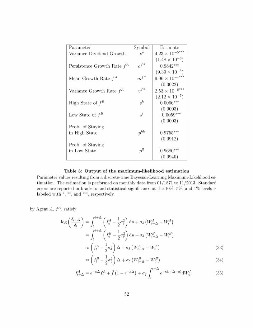
Parameter Symbol EstimateVariance Dividend Growth vδ 4.23× 10⁻⁵∗∗∗
(1.48× 10⁻⁶)
Persistence Growth Rate fA afA
0.9842∗∗∗
(9.39× 10⁻⁵)
Mean Growth Rate fA mfA 9.96× 10⁻⁴∗∗∗
(0.0022)
Variance Growth Rate fA vfA
2.53× 10⁻⁶∗∗∗
(2.12× 10⁻⁷)High State of fB sh 0.0066∗∗∗
(0.0003)Low State of fB sl −0.0059∗∗∗
(0.0003)Prob. of Stayingin High State phh 0.9755∗∗∗
(0.0912)Prob. of Stayingin Low State pll 0.9680∗∗∗
(0.0940)
Table 3: Output of the maximum-likelihood estimation
Parameter values resulting from a discrete-time Bayesian-Learning Maximum-Likelihood es-timation. The estimation is performed on monthly data from 01/1871 to 11/2013. Standarderrors are reported in brackets and statistical significance at the 10%, 5%, and 1% levels islabeled with ∗, ∗∗, and ∗∗∗, respectively.
by Agent A, fA, satisfy
log
(δt+∆
δt
)=
∫ t+∆
t
(fAu −
1
2σ2δ
)du+ σδ
(WAt+∆ −WA
t
)=
∫ t+∆
t
(fBu −
1
2σ2δ
)du+ σδ
(WBt+∆ −WB
t
)≈(fAt −
1
2σ2δ
)∆ + σδ
(WAt+∆ −WA
t
)(33)
≈(fBt −
1
2σ2δ
)∆ + σδ
(WBt+∆ −WB
t
)(34)
fAt+∆ = e−κ∆fAt + f(1− e−κ∆
)+ σf
∫ t+∆
te−κ(t+∆−u)dW f
u . (35)
52

The relationship between the transition matrix P and the generator matrix Λ is written as follows
P =
(phh 1− phh
1− pll pll
)(36)
=
(ψ
λ+ψ + λλ+ψe
−(λ+ψ)∆ λλ+ψ −
λλ+ψe
−(λ+ψ)∆
ψλ+ψ −
ψλ+ψe
−(λ+ψ)∆ λλ+ψ + ψ
λ+ψe−(λ+ψ)∆
).
We perform the Maximum-Likelihood estimation on monthly data and accordingly set ∆ = 112 =
1 month.Matching Eq. (30) to Eq. (33) and Eq. (31) to Eq. (35) yields the following system of equation
for κ, f , σδ, and σf
afA
= e−κ∆ (37)
mfA = f(1− e−κ∆
)− 1
2σ2δ∆
vδ = σ2δ∆
vfA
=σ2f
2κ
(1− e−2κ∆
),
where the last equation relates the variance of the Ornstein-Uhlenbeck process to its empiricalcounterpart. Matching Eq. (32) to Eq. (34) yields the following system of equations for f l and fh
sh =
(fh − 1
2σ2δ
)∆ (38)
sl =
(f l − 1
2σ2δ
)∆.
Solving the system comprised of Eqs. (36), (37), and (38) yields the parameters presented in Table1.
A.5 Conditional Distribution of the Filter
Agent A’s filter is (conditionally) normally distributed with mean mt = fA0 e−κt + f(1− e−κt) and
variance γ2
σ2δ
12κ(1 − e−2κt). Under Agent A’s probability measure and conditional on Agent A’s
filter being equal to its conditional mean mt, the conditional distribution PA(fBt |fAt = mt, fB0 ) =
p(fB, t; fA0 , fB0 ) of Agent B’s filter satisfies the Fokker-Planck equation
∂
∂tp = − ∂
∂fB
(p
1
dtEPAt [dfBt |fAt = mt]
)+
1
2
∂2
∂(fB)2
(p
1
dt(dfBt )2
)
53
with boundary conditions limfBfh p(f
B, t; fA0 , fB0 ) = lim
fBf l p(fB, t; fA0 , f
B0 ) = 0 and initial
condition p(fB, 0; fA0 , fB0 ) = δ
fB=fB0, where δ is the Dirac delta function. Boundary conditions are
derived in David (1997).
A.6 Proof of Proposition 3
The Malliavin derivative of the stock price satisfies
DtSu = EPAu
(∫ ∞u
[− ξsξ2u
δsDtξu +1
ξuδsDtξs +
ξsξuDtδs
]ds
). (39)
The definitions of the state-price density ξ, the dividend δ, the change of measure η, and the filterfA imply that
Dtξs = −αξsδsDtδs +
ξs(1− ω(ηs))
ηsDtηs (40)
Dtδs = δs
(σδ +
∫ s
tDtfAv dv
)(41)
Dtηs = − ηsσδ
(gt +
∫ s
tDtgvdWA
v +1
σδ
∫ s
tgvDtgvdv
)(42)
DtfAs =γ
σδe−κ(s−t). (43)
Substituting Eq. (43) in Eq. (41) yields
Dtδsδs
= σδ +γ
κσδ
(1− e−κ(s−t)
), (44)
while substituting Eqs. (41), (42), and (43) in Eq. (40) yields
Dtξsξs
= −α(σδ +
γ
κσδ
(1− e−κ(s−t)
))− 1− ω(ηs)
σδ
(gt +
∫ s
tDtgvdWA
v +1
σδ
∫ s
tgvDtgvdv
).
(45)
54
Then, substituting Eqs. (44) and (45) in Eq. (39) yields
DtSu = σδSu +γ
κσδ
((1− αe−κ(u−t)
)Su + (α− 1)EPA
u
[∫ ∞u
ξsξuδse−κ(s−t)ds
])+
1
σ2δ
(Su(1− ω(ηu))
∫ u
tgvDtgvdv − EPA
u
(∫ ∞u
ξsξuδs(1− ω(ηs))
∫ s
tgvDtgvdvds
))+
1− ω(ηu)
σδSu
(gt +
∫ u
tDtgvdWA
v
)− 1
σδEPAu
(∫ ∞u
ξsξuδs(1− ω(ηs))
(gt +
∫ s
tDtgvdWA
v
)ds
).
(46)
Taking conditional expectation at time t and setting gt = 0 implies that the last line of Eq. (46)vanishes. That is,
EPAt (DtSu) = σδEPA
t (Su) +γ
κσδ
((1− αe−κ(u−t)
)EPAt (Su) + (α− 1)EPA
t
[∫ ∞u
ξsξuδse−κ(s−t)ds
])
+1
σ2δ
EPAt
(∫ ∞u
ξsξuδs
((ω(ηs)− ω(ηu))
∫ u
tgvDtgvdv − (1− ω(ηs))
∫ s
ugvDtgvdv
)ds
).
A.7 Proof of Proposition 5
The dynamics of Agent A’s wealth satisfy
dVt = rft Vtdt+(µt − rft
)QtStdt− cAtdt+ σtQtStdW
At , (47)
where rf is the risk-free rate defined in Eq. (9), µ− rf is the risk premium on the stock, Q is thenumber of shares held by Agent A, and σ is the diffusion of stock returns.
Applying Ito’s lemma to the stock price yields the diffusion of stock returns, σ, as follows:
σ = σδ +DfA
γ
σδ+Dg
γ −(fA − g − f l
)(fh + g − fA
)σδ
−Dηgη
σδ,
where Dx ≡ 1S∂S∂x .
The risk premium, µ− rf , satisfies
µ− rf = σθ,
where σ and θ are defined in Eqs. (16) and (10), respectively.
55

Applying Ito’s lemma to Agent A’s wealth and matching resulting diffusion term with that inEq. (47) gives the number of shares held by Agent A, Q, which satisfies
Q =Vδσδδ + V
fAγσδ
+ Vgγ−(fA−g−f l)(fh+g−fA)
σδ− Vη gησδ
σS,
where Vx ≡ ∂V∂x . To quantify the profit generated by exploiting exclusively predictability, we break
the number of shares into two components, as follows:
Q ≡M +H,
where M is the myopic component and H the hedging component. We characterize the myopic andthe hedging components using the Martingale Representation Theorem along with the Clark-OconeTheorem. Specifically, we define the following martingale
d
(ξtVt +
∫ t
0ξscAsds
)= φtdW
At
= EPAt
(∫ ∞tDt (ξscAs) ds
)dWA
t
= (ξtσtQtSt − Vtθtξt) dWAt ,
where the first and second equalities follow from the Martingale Representation Theorem and theClark-Ocone Theorem, respectively. Therefore, the number of shares Q satisfies
Qt =µt − rftσ2t
VtSt
+1
ξtσtStEPAt
(∫ ∞tDt (ξscAs) ds
). (48)
Using the fact that
ξscAs = (φAeρs)−1/α ξ
α−1α
s and thus
Dt (ξscAs) =α− 1
αDt(ξs)cAs,
56

we can rewrite Eq. (48) as follows
Qt =µt − rftσ2t
VtSt
+α− 1
ασtStEPAt
(∫ ∞t
ξscAsξt
Dtξsξs
ds
)=µt − rftσ2t
VtSt
+α− 1
ασtStEPAt
(∫ ∞t
ξscAsξt
(Dtξsξs− Dtξt
ξt+Dtξtξt
)ds
)=µt − rftσ2t
VtSt
+α− 1
ασtStEPAt
(∫ ∞t
ξscAsξt
(Dtξsξs− Dtξt
ξt
)ds
)− (α− 1)θtVt
ασtSt
=µt − rftασ2
t
VtSt
+α− 1
ασtStEPAt
(∫ ∞t
ξscAsξt
(Dtξsξs− Dtξt
ξt
)ds
)≡Mt +Ht.
57