Embed Size (px)
Citation preview
©Product Ventures, Inc., March, 2015 1
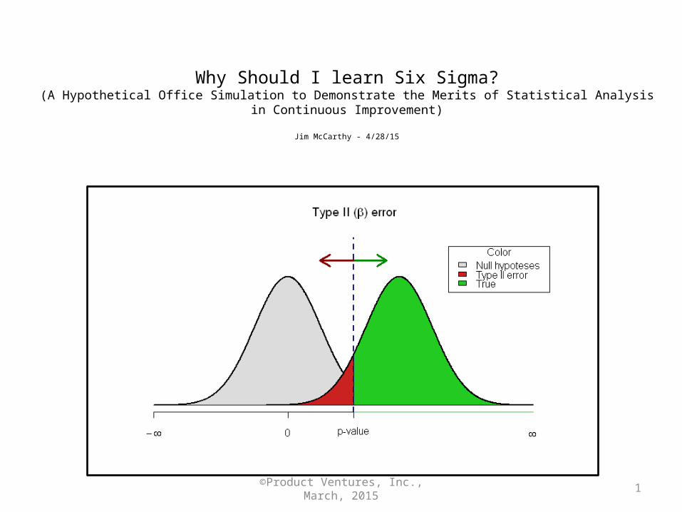
Why Should I learn Six Sigma?(A Hypothetical Office Simulation to Demonstrate the Merits of Statistical Analysis in Continuous Improvement)
Jim McCarthy - 4/28/15
©Product Ventures, Inc., March, 2015 2
Agenda1. CEO wants customer quoting issues resolved fast2. I am selected to get it done3. Initial known facts & data4. Conventional thinking & methods5. Capability Study6. Analysis of Variance (ANOVA) & Std. Dev. Test 7. Charter: Deliverables, Team, Gantt Chart, Scope,
Dates, Report-Out/s, Process Analyses, etc.8. Design of Experiments (DOE)9. Possible solutions

©Product Ventures, Inc., March, 2015 3
How It Started
CEO receives phone calls from customers:“You are not providing quotes in a timely manner!”
Customers threaten to go to a competitor
Global Customer Base
(All Time Zones)
©Product Ventures, Inc., March, 2015 4
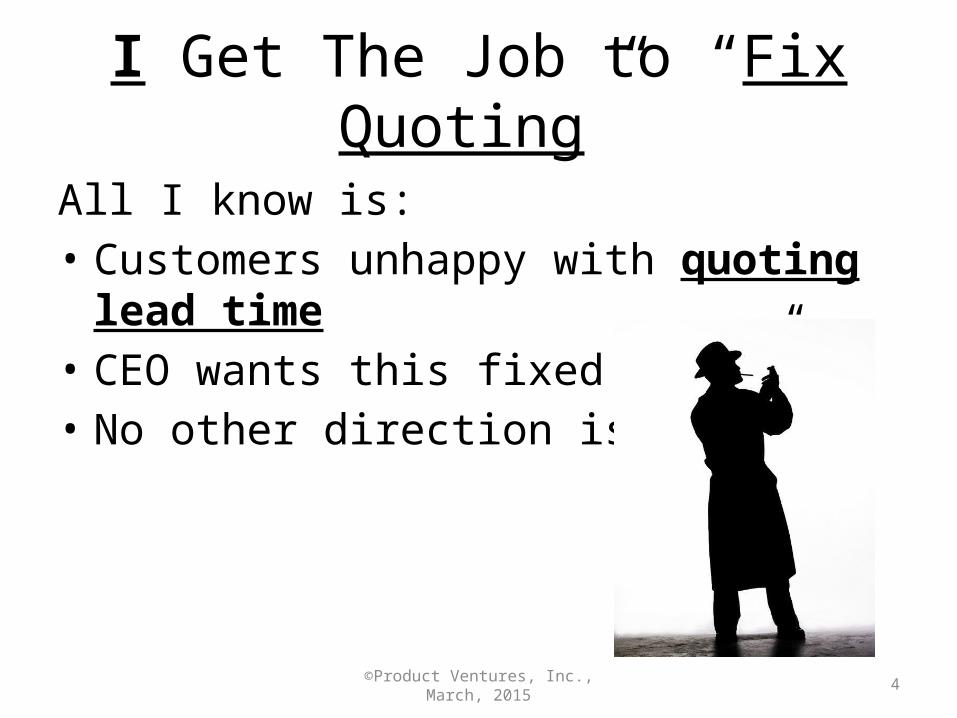
I Get The Job to “Fix Quoting”
All I know is: • Customers unhappy with quoting lead time• CEO wants this fixed “Fast”• No other direction is given
©Product Ventures, Inc., March, 2015 5
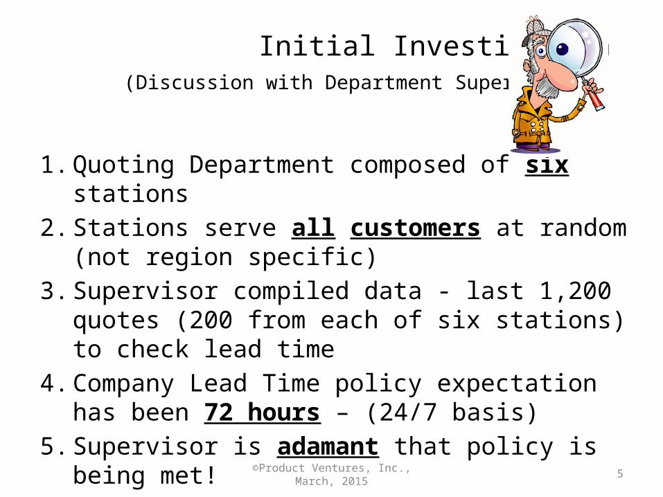
Initial Investigation (Discussion with Department Supervisor)
1. Quoting Department composed of six stations2. Stations serve all customers at random (not
region specific)3. Supervisor compiled data - last 1,200 quotes
(200 from each of six stations) to check lead time4. Company Lead Time policy expectation has been
72 hours – (24/7 basis) 5. Supervisor is adamant that policy is being met!
©Product Ventures, Inc., March, 2015 6
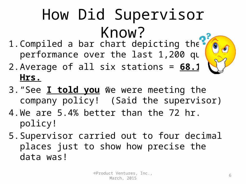
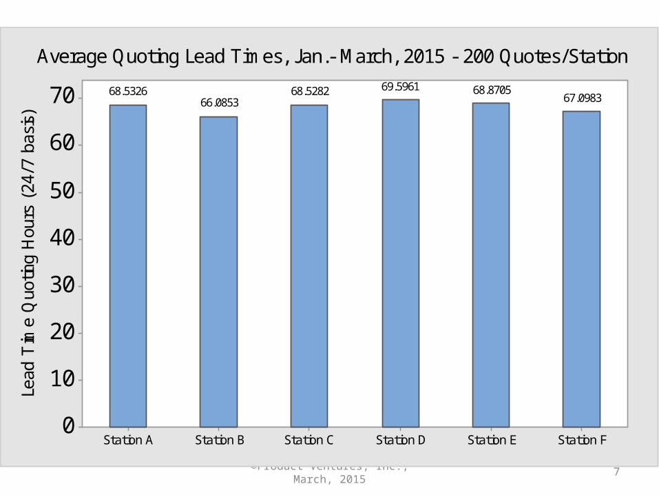
How Did Supervisor Know?1. Compiled a bar chart depicting the
performance over the last 1,200 quotes2. Average of all six stations = 68.1185 Hrs.3. “See I told you we were meeting the company
policy!” (Said the supervisor)4. We are 5.4% better than the 72 hr. policy!5. Supervisor carried out to four decimal places
just to show how precise the data was!
©Product Ventures, Inc., March, 2015 7
Station FStation EStation DStation CStation BStation A
70
60
50
40
30
20
10
0
Lead
Tim
e Q
uotin
g H
ours
(24
/7 b
asis)
68.532666.0853
68.5282 69.5961 68.870567.0983
Average Quoting Lead Times, Jan.- March, 2015 - 200 Quotes/Station
©Product Ventures, Inc., March, 2015 8
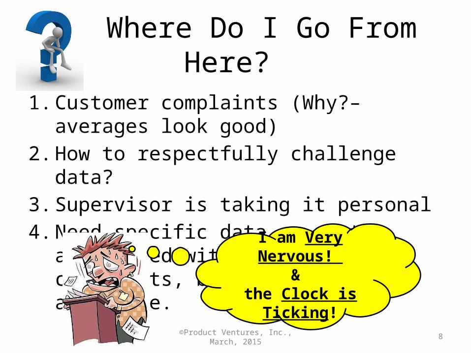
Where Do I Go From Here?
1. Customer complaints (Why?–averages look good)2. How to respectfully challenge data?3. Supervisor is taking it personal 4. Need specific data on quotes associated with
customer complaints, but data is not available.
I am Very Nervous! &
the Clock is Ticking!
©Product Ventures, Inc., March, 2015 9
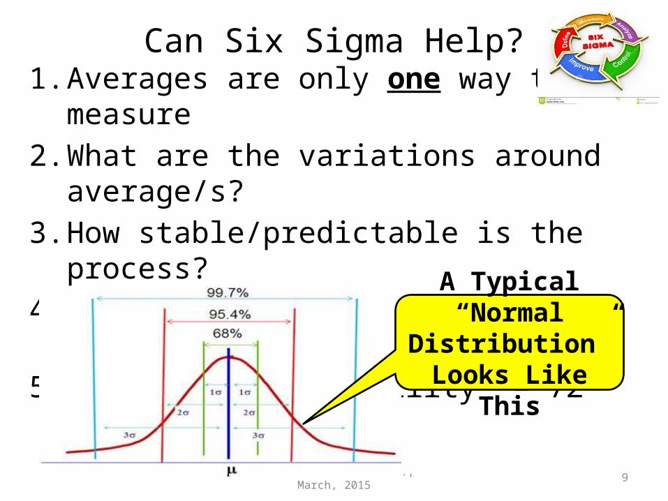
Can Six Sigma Help?1. Averages are only one way to measure2. What are the variations around average/s?3. How stable/predictable is the process?4. Are all quoting stations statistically similar?5. Does system “Capability” = 72 hours or less?
A Typical “Normal Distribution”
Looks Like This
©Product Ventures, Inc., March, 2015 10
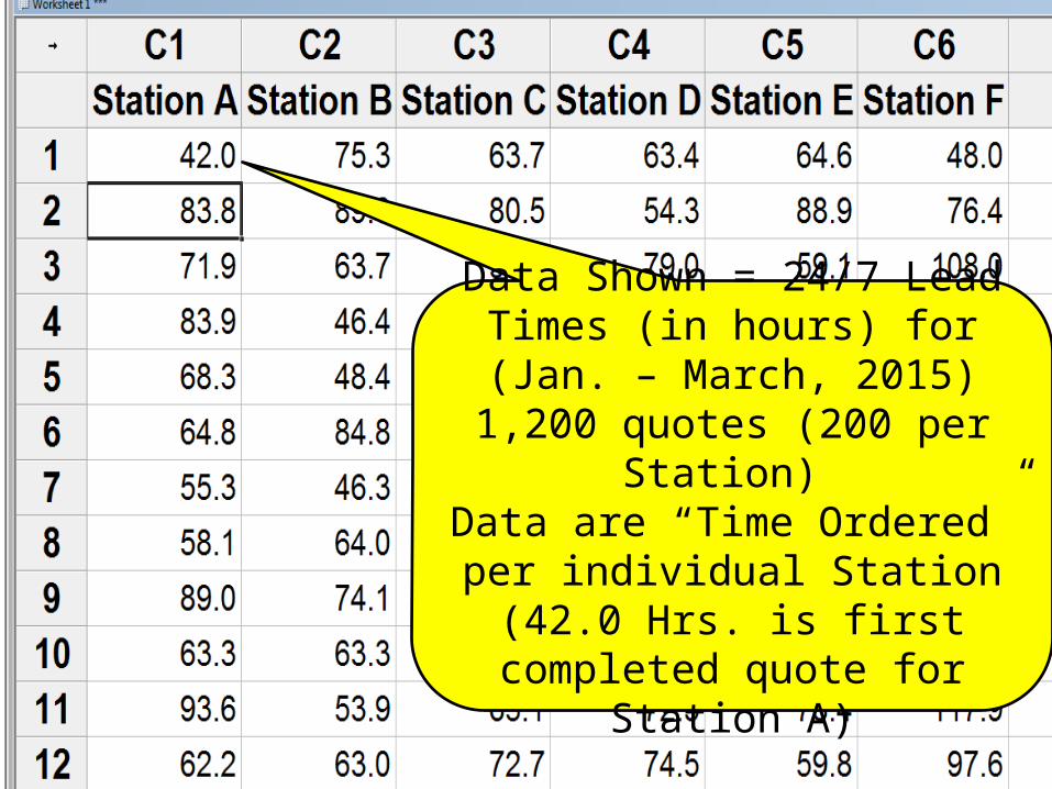
Data Shown = 24/7 Lead Times (in hours) for (Jan. – March, 2015)1,200 quotes (200 per Station) Data are “Time Ordered” per
individual Station (42.0 Hrs. is first completed quote for Station A)
©Product Ventures, Inc., March, 2015 11
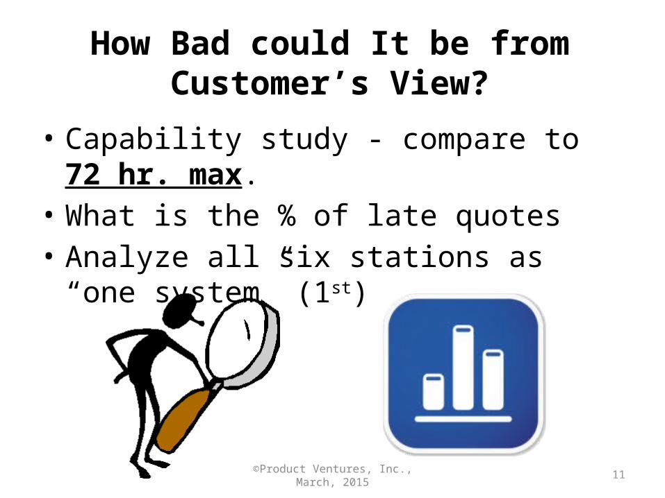
How Bad could It be from Customer’s View?
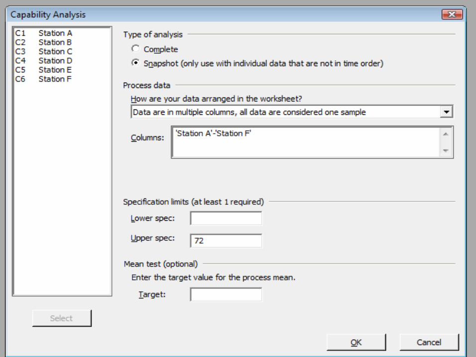
• Capability study - compare to 72 hr. max. • What is the % of late quotes• Analyze all six stations as “one system” (1st)
©Product Ventures, Inc., March, 2015 12
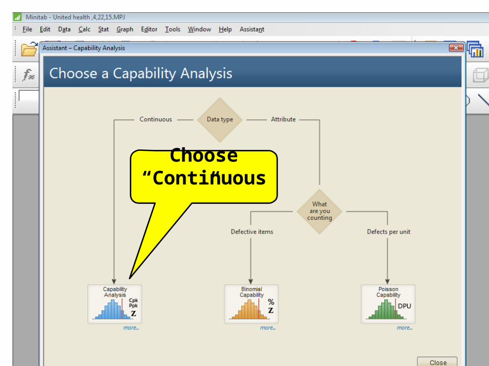
Choose “Continuous”
©Product Ventures, Inc., March, 2015 13
©Product Ventures, Inc., March, 2015 14
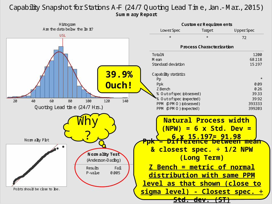
Normality Test
Results FailP-value 0.005
(Anderson-Darling)
Customer RequirementsLower Spec Target Upper Spec
* * 72
% Out of spec (expected) 39.92 PPM (DPMO) (observed) 393333 PPM (DPMO) (expected) 399203
Total N 1200Mean 68.118Standard deviation 15.197
Capability statistics Pp * Ppk 0.09 Z.Bench 0.26 % Out of spec (observed) 39.33
Process Characterization
14012010080604020
Quoting Lead time (24/7 Hrs.)
USL
measures represent long-term performance, may not apply.time. Therefore, the usual interpretation, that the capabilitysources of variation that may appear over a longer period ofHowever, the data collection method used may not capture allThe capability measures use the overall standard deviation.
HistogramAre the data below the limit?
Normality Plot
Points should be close to line.
Comments
Capability Snapshot for Stations A-F (24/7 Quoting Lead Time, Jan.- Mar., 2015)Summary Report
Natural Process width (NPW) = 6 x Std. Dev = 6 x 15.197= 91.98
39.9% Ouch!
Ppk = Difference between mean & closest spec. ÷ 1/2 NPW (Long Term)
Z Bench = metric of normal distribution with same PPM level as that shown (close to
sigma level) - Closest spec. ÷ Std. dev. (ST)
Why?
©Product Ventures, Inc., March, 2015 15
10
5
01
51
02
52
03
53
02 04 06 08 001 021 04
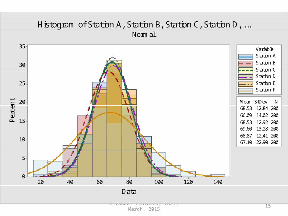
68.53 12.84 20066.09 14.02 20068.53 12.92 20069.60 13.28 20068.87 12.41 20067.10 22.90 200
Mean StDev N
D
tnecreP
ata
SelbairaV
F noitatSE noitatSD noitatSC noitatSB noitatSA noitat
H lamroN
... ,D noitatS ,C noitatS ,B noitatS ,A noitatS fo margotsi
©Product Ventures, Inc., March, 2015 16
1501251007550250
99.9
99
95
90
80706050403020
10
5
1
0.1
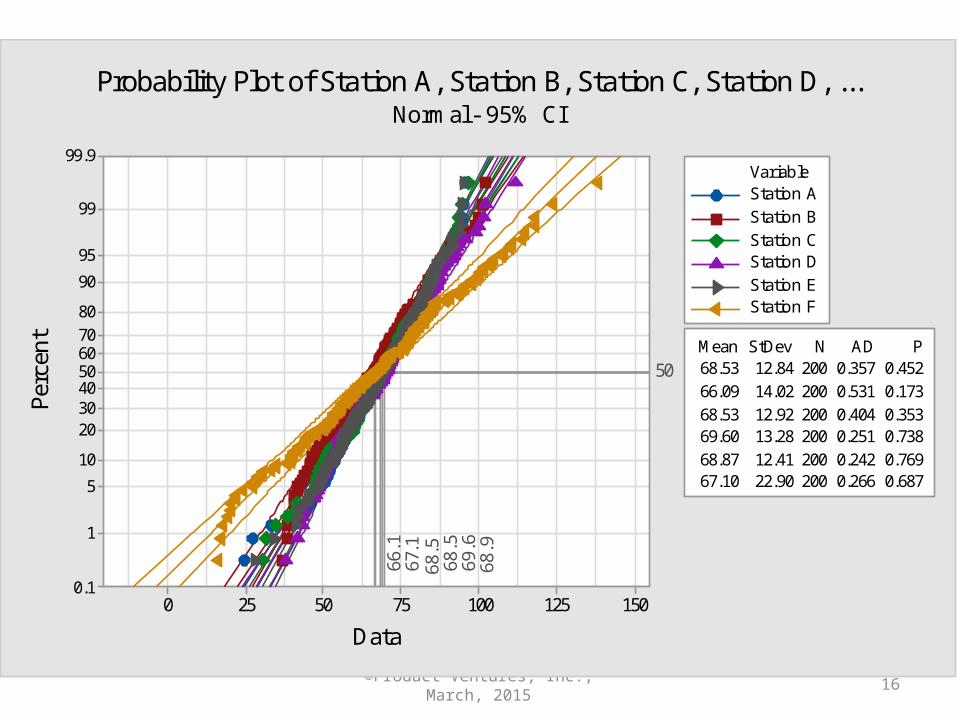
68.53 12.84 200 0.357 0.45266.09 14.02 200 0.531 0.17368.53 12.92 200 0.404 0.35369.60 13.28 200 0.251 0.73868.87 12.41 200 0.242 0.76967.10 22.90 200 0.266 0.687
Mean StDev N AD P
Data
Perc
ent
68.5
66.1
68.5
69.6
68.9
67.1
50
Station AStation BStation CStation DStation EStation F
Variable
Probability Plot of Station A, Station B, Station C, Station D, ...Normal - 95% CI
©Product Ventures, Inc., March, 2015 17
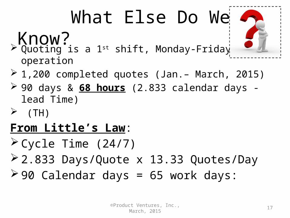
What Else Do We Know? Quoting is a 1st shift, Monday-Friday operation 1,200 completed quotes (Jan.– March, 2015) 90 days & 68 hours (2.833 calendar days - lead Time) (TH)
From Little’s Law: Cycle Time (24/7) 2.833 Days/Quote x 13.33 Quotes/Day 90 Calendar days = 65 work days:

©Product Ventures, Inc., March, 2015 18
Need to Be “Data Driven”!1. What is present incoming rate from customer?2. Visual daily metrics & “stand-up” meetings (10
minutes) for: Cycle Time, Throughput, & WIP3. Can’t improve (or manage) what we don’t measure!
©Product Ventures, Inc., March, 2015 19
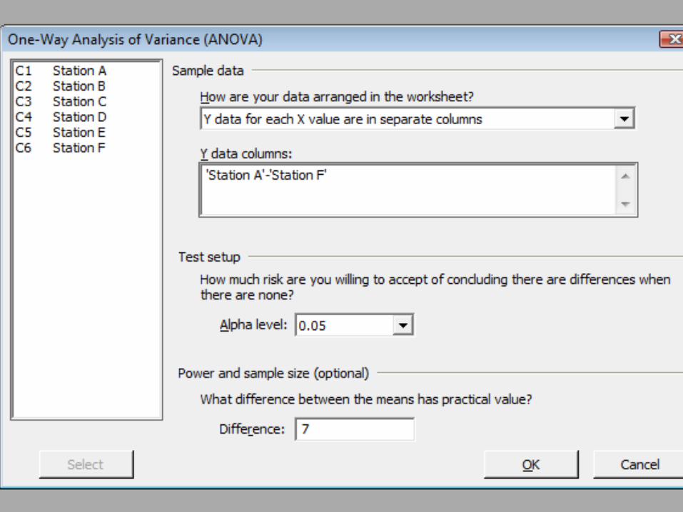
Let’s Dig DeeperAnalysis of Variance (ANOVA)
• 6 Sigma tool (comparison-multiple data sets)• ANOVA tries to determine if all data sets are from the same
population• Looks at both the mean (average) & variation of all data sets• Develops a ratio of the “between” data groups to “within”
each data group. • Calculates an “F” ratio & compares it to a critical value to
determine if the null hypothesis (data is statistically the same) can be rejected
• 1st – ANOVA assumes “Normal” data – need to check
©Product Ventures, Inc., March, 2015 20
ANOVA
• Between-Groups Variance (BGV)• Within Groups Variance (WGV)
• If the “F” ratio is larger than “F critical” then we reject the null hypothesis because we cannot be sure that all data sets are from the same population.
• ANOVA requires significant calculations and is best done using software.
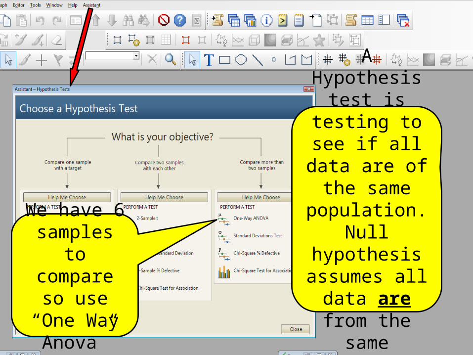
©Product Ventures, Inc., March, 2015 21
We have 6 samples to compare so
use “One Way Anova”
A Hypothesis test is testing to
see if all data are of the same
population.Null hypothesis assumes all data
are from the same population
©Product Ventures, Inc., March, 2015 22
©Product Ventures, Inc., March, 2015 23
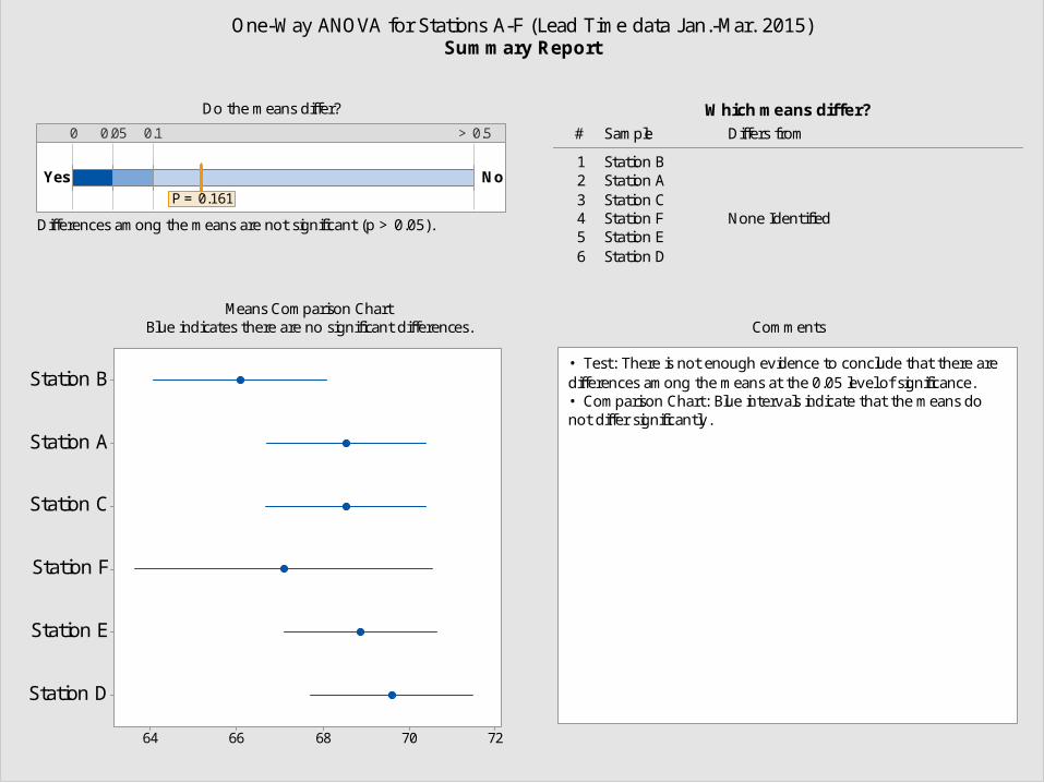
Which means differ?
1 Station B2 Station A3 Station C4 Station F None Identified5 Station E6 Station D
# Sample Differs from
Differences among the means are not significant (p > 0.05).
Yes No
0 0.05 0.1 > 0.5
P = 0.161
Station D
Station E
Station F
Station C
Station A
Station B
7270686664
not differ significantly.• Comparison Chart: Blue intervals indicate that the means dodifferences among the means at the 0.05 level of significance.• Test: There is not enough evidence to conclude that there are
Do the means differ?
Means Comparison ChartBlue indicates there are no significant differences. Comments
One-Way ANOVA for Stations A-F (Lead Time data J an.-Mar. 2015)Summary Report
©Product Ventures, Inc., March, 2015 24
©Product Ventures, Inc., March, 2015 25
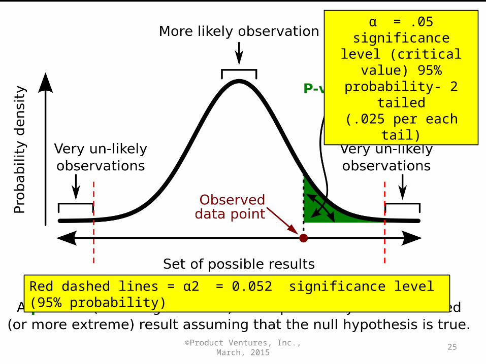
Red dashed lines = α2 = 0.052 significance level (95% probability)
α = .05 significance level (critical value) 95% probability- 2 tailed(.025 per each tail)
©Product Ventures, Inc., March, 2015 26
100
50
0
100
50
0
100
50
0
Station A Station B
Station C Station D
Station E Station F
14012010080604020
Station A
Station B
Station C
Station D
Station E
Station F
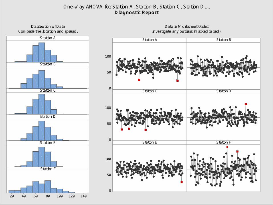
Data in Worksheet OrderInvestigate any outliers (marked in red).
Distribution of DataCompare the location and spread.
One-Way ANOVA for Station A, Station B, Station C, Station D,...Diagnostic Report
©Product Ventures, Inc., March, 2015 27
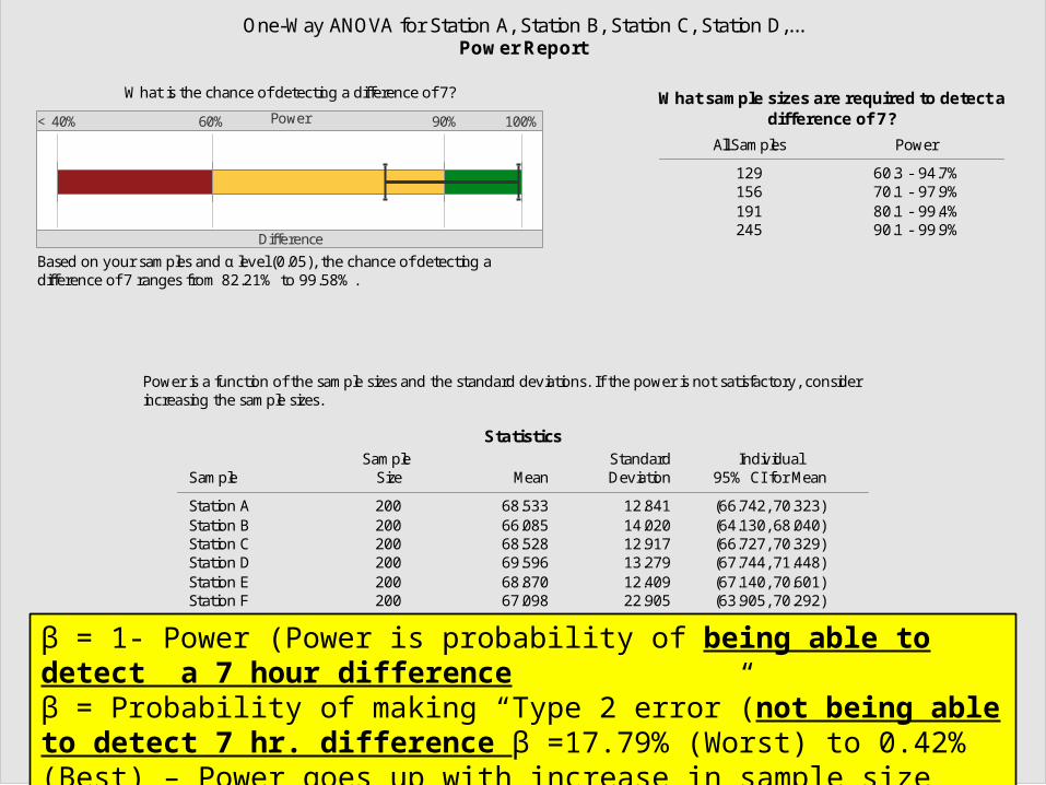
difference of 7?What sample sizes are required to detect a
129 60.3 - 94.7%156 70.1 - 97.9%191 80.1 - 99.4%245 90.1 - 99.9%
All Samples Power
Statistics
Station A 200 68.533 12.841 (66.742, 70.323)Station B 200 66.085 14.020 (64.130, 68.040)Station C 200 68.528 12.917 (66.727, 70.329)Station D 200 69.596 13.279 (67.744, 71.448)Station E 200 68.870 12.409 (67.140, 70.601)Station F 200 67.098 22.905 (63.905, 70.292)
Sample SizeSample
Mean DeviationStandard
95% CI for MeanIndividual
difference of 7 ranges from 82.21% to 99.58%.Based on your samples and α level (0.05), the chance of detecting a
Difference
Power< 40% 60% 90% 100%
What is the chance of detecting a difference of 7?
increasing the sample sizes.Power is a function of the sample sizes and the standard deviations. If the power is not satisfactory, consider
One-Way ANOVA for Station A, Station B, Station C, Station D,...Power Report
β = 1- Power (Power is probability of being able to detect a 7 hour differenceβ = Probability of making “Type 2 error”(not being able to detect 7 hr. difference β =17.79% (Worst) to 0.42% (Best) – Power goes up with increase in sample size
©Product Ventures, Inc., March, 2015 28
Station F
Station E
Station D
Station C
Station B
Station A
28262422201816141210
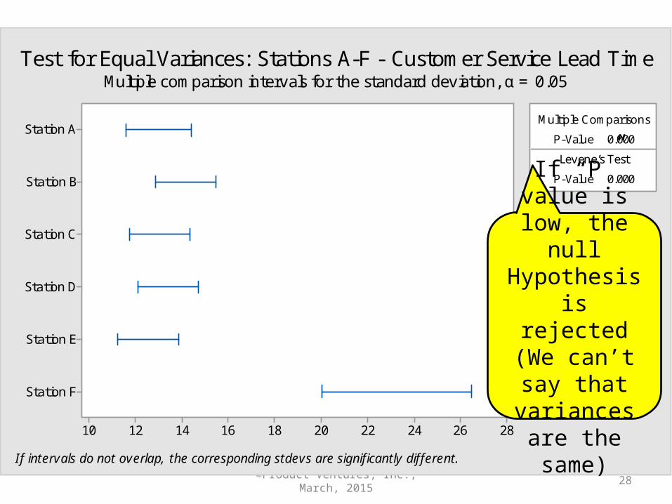
P-Value 0.000
P-Value 0.000
Multiple Comparisons
Levene’s Test
Test for Equal Variances: Stations A-F - Customer Service Lead TimeMultiple comparison intervals for the standard deviation, α = 0.05
If intervals do not overlap, the corresponding stdevs are significantly different.
If “P” value is low, the null Hypothesis is
rejected(We can’t say that variances are the same)
©Product Ventures, Inc., March, 2015 29
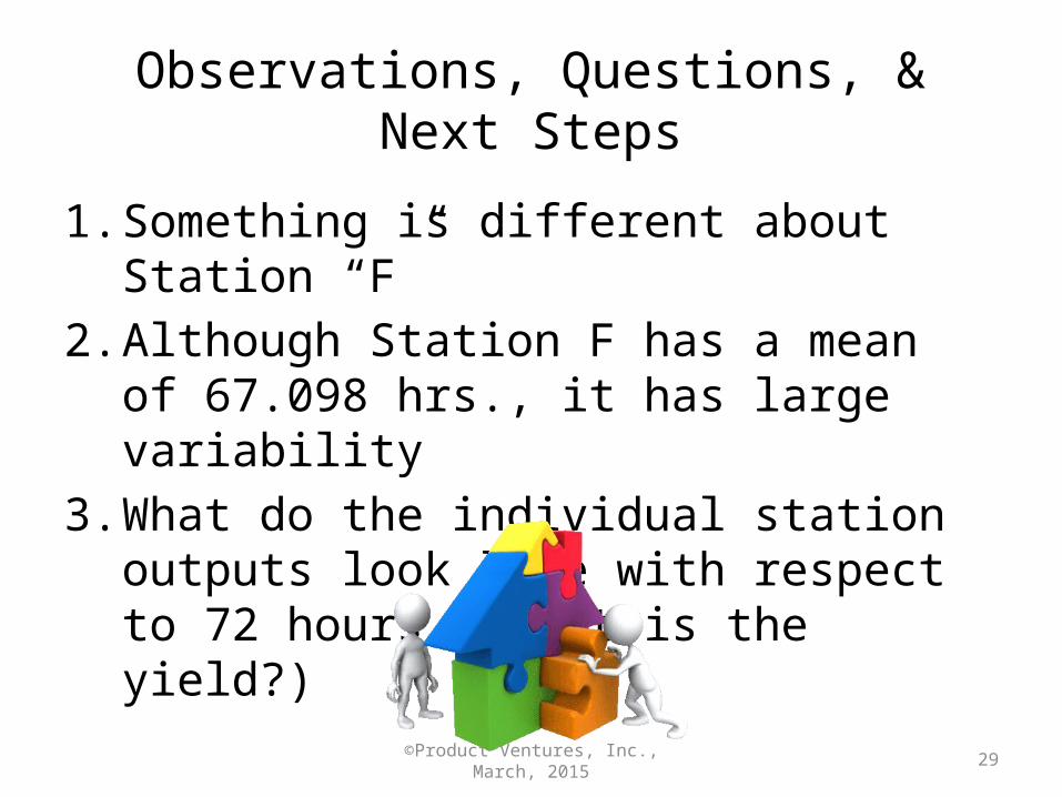
Observations, Questions, & Next Steps
1. Something is different about Station “F”2. Although Station F has a mean of 67.098 hrs.,
it has large variability3. What do the individual station outputs look
like with respect to 72 hours ( What is the yield?)
©Product Ventures, Inc., March, 2015 30
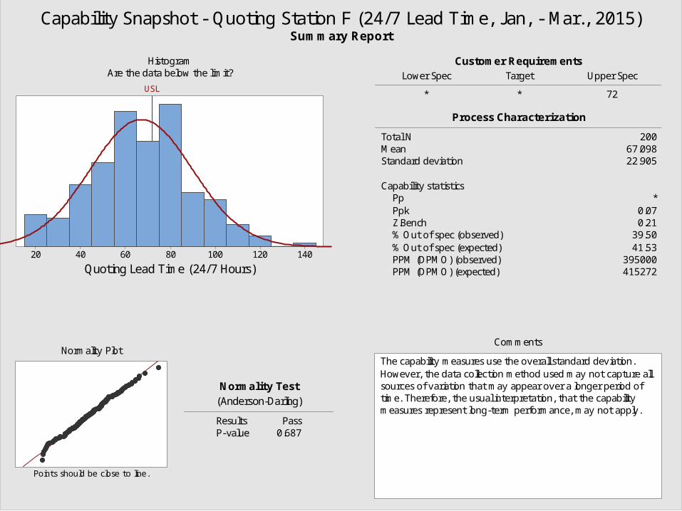
Normality Test
Results PassP-value 0.687
(Anderson-Darling)
Customer RequirementsLower Spec Target Upper Spec
* * 72
% Out of spec (expected) 41.53 PPM (DPMO) (observed) 395000 PPM (DPMO) (expected) 415272
Total N 200Mean 67.098Standard deviation 22.905
Capability statistics Pp * Ppk 0.07 Z.Bench 0.21 % Out of spec (observed) 39.50
Process Characterization
14012010080604020
Quoting Lead Time (24/7 Hours)
USL
measures represent long-term performance, may not apply.time. Therefore, the usual interpretation, that the capabilitysources of variation that may appear over a longer period ofHowever, the data collection method used may not capture allThe capability measures use the overall standard deviation.
HistogramAre the data below the limit?
Normality Plot
Points should be close to line.
Comments
Capability Snapshot - Quoting Station F (24/7 Lead Time, Jan, - Mar., 2015)Summary Report
©Product Ventures, Inc., March, 2015 31
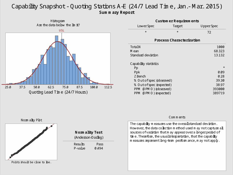
Normality Test
Results PassP-value 0.494
(Anderson-Darling)
Customer RequirementsLower Spec Target Upper Spec
* * 72
% Out of spec (expected) 38.97 PPM (DPMO) (observed) 393000 PPM (DPMO) (expected) 389719
Total N 1000Mean 68.323Standard deviation 13.132
Capability statistics Pp * Ppk 0.09 Z.Bench 0.28 % Out of spec (observed) 39.30
Process Characterization
112.5100.087.575.062.550.037.525.0
Quoting Lead Time (24/7 Hours)
USL
measures represent long-term performance, may not apply.time. Therefore, the usual interpretation, that the capabilitysources of variation that may appear over a longer period ofHowever, the data collection method used may not capture allThe capability measures use the overall standard deviation.
HistogramAre the data below the limit?
Normality Plot
Points should be close to line.
Comments
Capability Snapshot - Quoting Stations A-E (24/7 Lead Time, Jan.- Mar. 2015)Summary Report
©Product Ventures, Inc., March, 2015 32
What Next?1. Station “F” has high variability & is not capable (41.53% failure rate
for 72 hr. Spec.)2. “A-F” have a 39.92% (collective) failure rate (not capable)3. “A-E” have 38.97 (collective) failure rate (not capable)4. This requires a systemic change to reduce common cause
variability & reduce “mean” across all stations.5. Write a charter, form a team, get understanding & agreement from
management , & write project plan 6. Spend some time investigating Station “F” variance in order to
better understand process. (DOE)7. Do “Data Tagging” & value stream map (I.D. waste)8. I.D. working hours, shifts, RFQ input rate, departments, etc.9. Design & review daily metrics charts: WIP, Throughput, 24/7 Cycle
Time, & Quality Issues
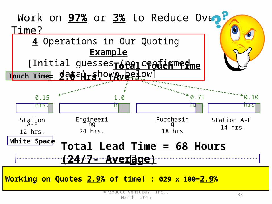
©Product Ventures, Inc., March, 2015 33
Touch Time
White Space
Working on Quotes 2.9% of time! : 029 x 100=2.9%
0.15 hrs. 1.0 hrs. 0.75 hrs. 0.10 hrs.
Station A-F12 hrs.
Engineering24 hrs.
Purchasing18 hrs
Station A-F 14 hrs.
Total Lead Time = 68 Hours (24/7- Average)
Work on 97% or 3% to Reduce Overall Time?
Total Touch Time = 2.0 Hrs. (Ave.)
4 Operations in Our Quoting Example[Initial guesses (no confirmed data) shown below]
©Product Ventures, Inc., March, 2015 34
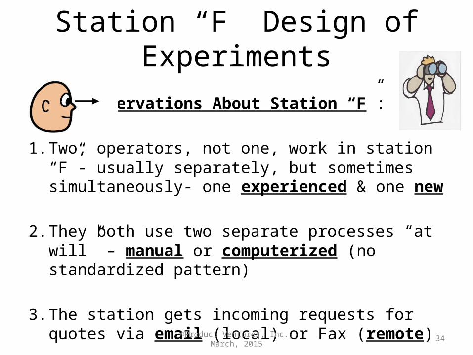
Station “F” Design of Experiments
Observations About Station “F”:
1. Two, operators, not one, work in station “F”- usually separately, but sometimes simultaneously- one experienced & one new
2. They both use two separate processes “at will” – manual or computerized (no standardized pattern)
3. The station gets incoming requests for quotes via email (local) or Fax (remote)
©Product Ventures, Inc., March, 2015 35
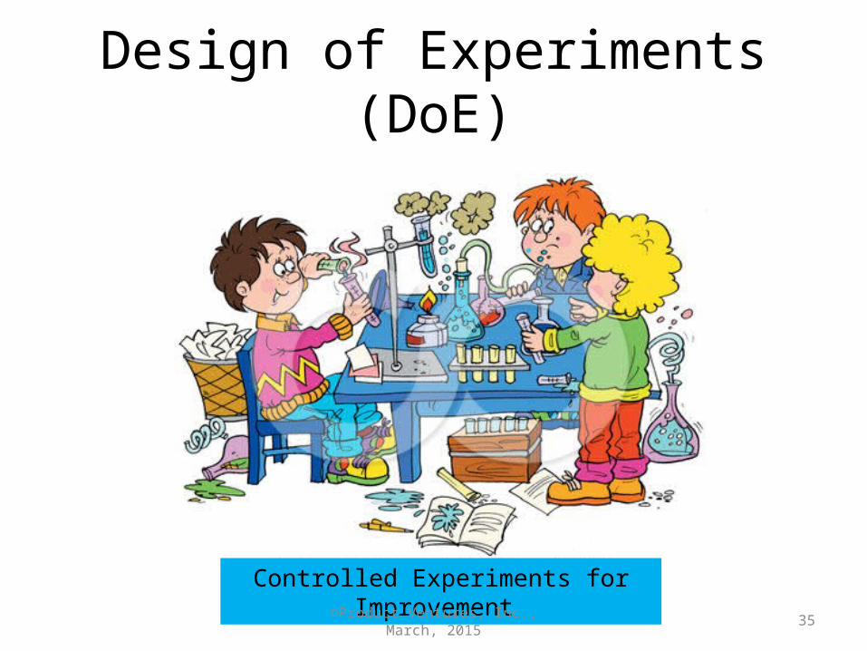
Design of Experiments (DoE)
Controlled Experiments for Improvement
©Product Ventures, Inc., March, 2015 36
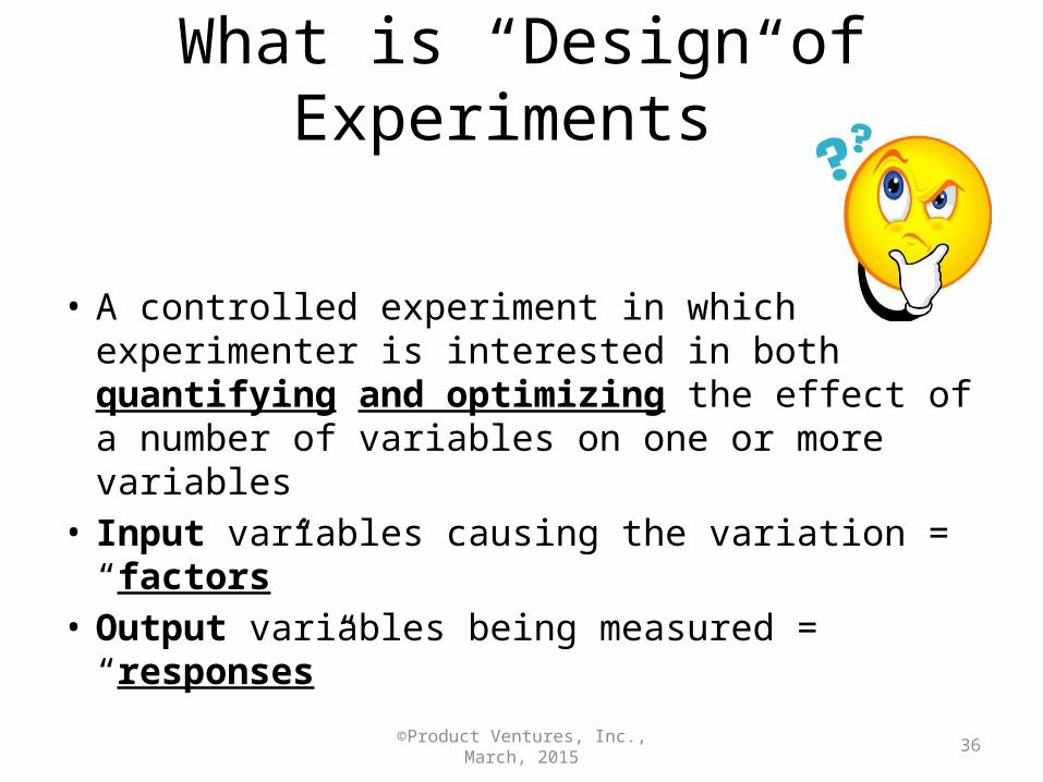
What is “Design of Experiments”
• A controlled experiment in which the experimenter is interested in both quantifying and optimizing the effect of a number of variables on one or more variables
• Input variables causing the variation = “factors”• Output variables being measured = “responses”
©Product Ventures, Inc., March, 2015 37
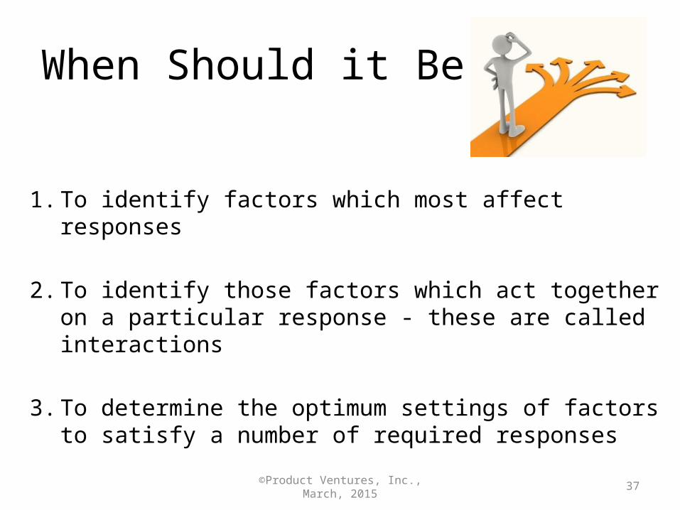
When Should it Be Used?
1. To identify factors which most affect responses
2. To identify those factors which act together on a particular response - these are called interactions
3. To determine the optimum settings of factors to satisfy a number of required responses
©Product Ventures, Inc., March, 2015 38
DOE Basics
• Follows the 6 sigma transfer function:
Which means that “Y” (output or response) is equal to a function of the “X” input/s (factors)
©Product Ventures, Inc., March, 2015 39
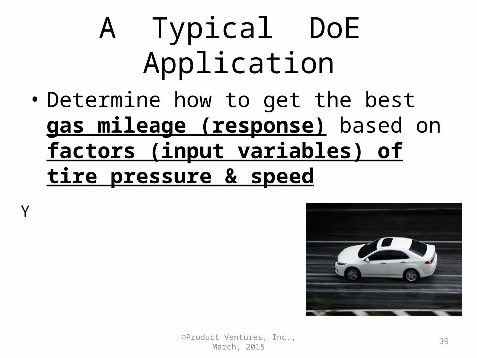
A Typical DoE Application
• Determine how to get the best gas mileage (response) based on factors (input variables) of tire pressure & speed
Y
©Product Ventures, Inc., March, 2015 40
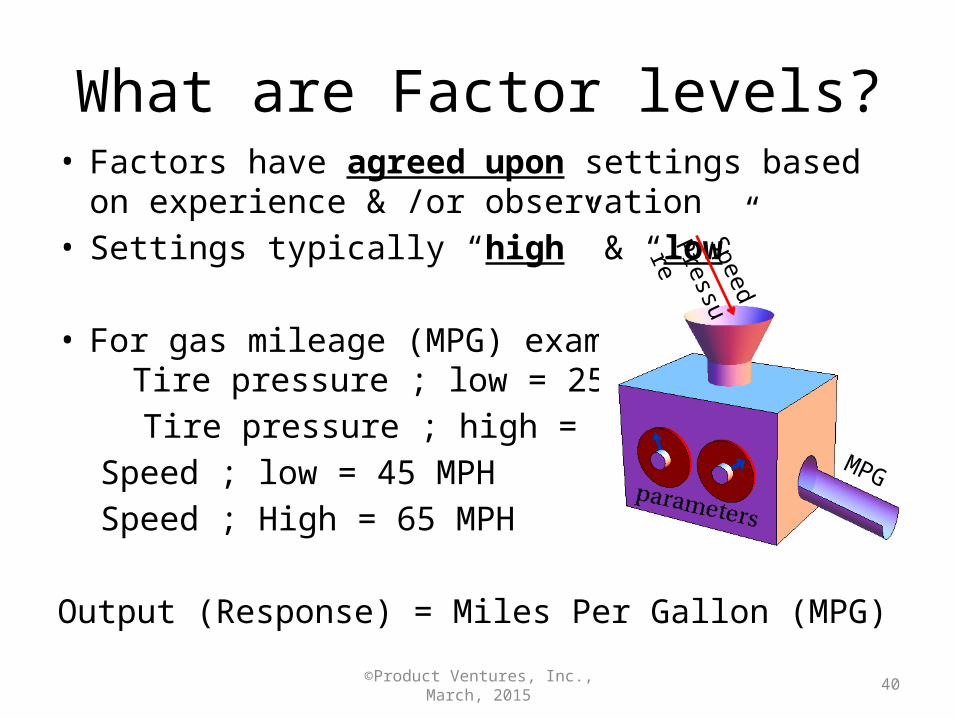
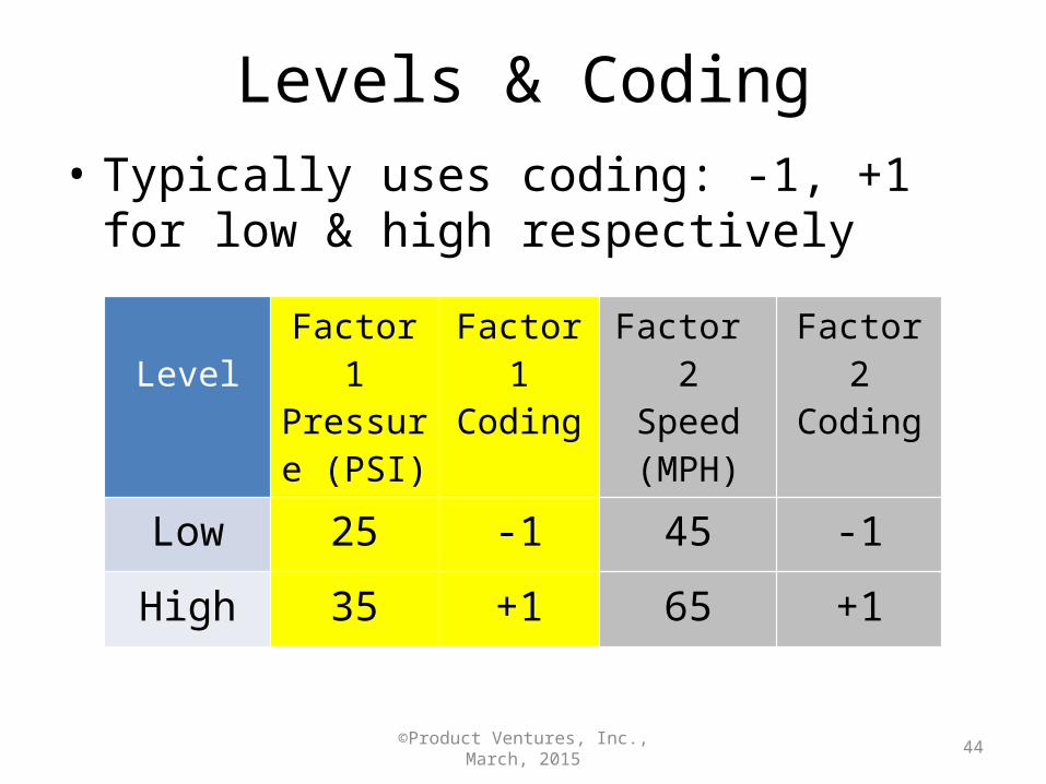
What are Factor levels?• Factors have agreed upon settings based on experience &
/or observation• Settings typically “high” & “low”
• For gas mileage (MPG) example:Tire pressure ; low = 25 Psi
Tire pressure ; high = 35 PsiSpeed ; low = 45 MPHSpeed ; High = 65 MPH
Output (Response) = Miles Per Gallon (MPG)
Speed
Pressure
MPG
©Product Ventures, Inc., March, 2015 41
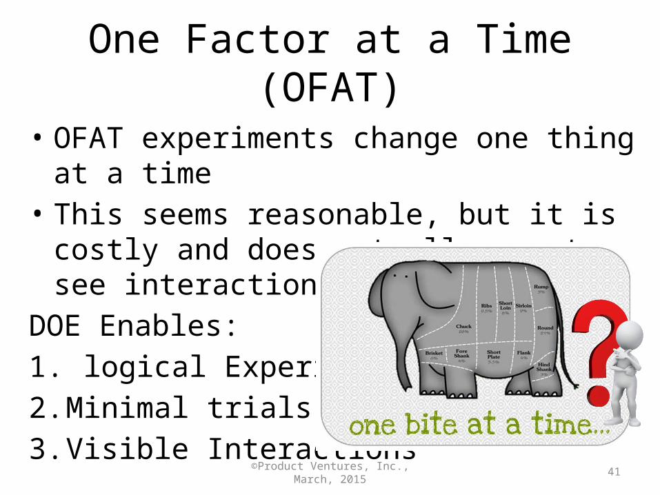
One Factor at a Time (OFAT)
• OFAT experiments change one thing at a time• This seems reasonable, but it is costly and does
not allow us to see interactions between inputsDOE Enables:1. logical Experiments2. Minimal trials3. Visible Interactions
©Product Ventures, Inc., March, 2015 42
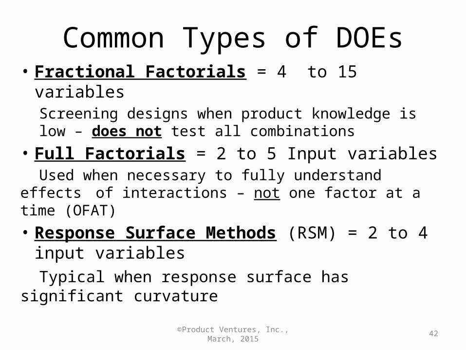
Common Types of DOEs• Fractional Factorials = 4 to 15 variables
Screening designs when product knowledge is low – does not test all combinations
• Full Factorials = 2 to 5 Input variablesUsed when necessary to fully understand effects
of interactions – not one factor at a time (OFAT)• Response Surface Methods (RSM) = 2 to 4
input variablesTypical when response surface has significant
curvature
©Product Ventures, Inc., March, 2015 43
DOE Notation
• General notation used to designate a full factorial design is shown as:
• Where k is the number of input variables or factors
• 2 = the number of “levels” that will be used for each factor
©Product Ventures, Inc., March, 2015 44
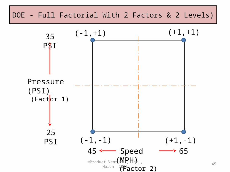
Levels & Coding• Typically uses coding: -1, +1 for low & high
respectively
LevelFactor 1 Pressure
(PSI)
Factor 1Coding
Factor 2Speed(MPH)
Factor 2Coding
Low 25 -1 45 -1
High 35 +1 65 +1
©Product Ventures, Inc., March, 2015 45
DOE - Full Factorial With 2 Factors & 2 Levels)
Pressure (PSI)(Factor 1)
25 PSI
35 PSI
Speed (MPH)(Factor 2)
45 65
(-1,+1) (+1,+1)
(-1,-1) (+1,-1)
©Product Ventures, Inc., March, 2015 46
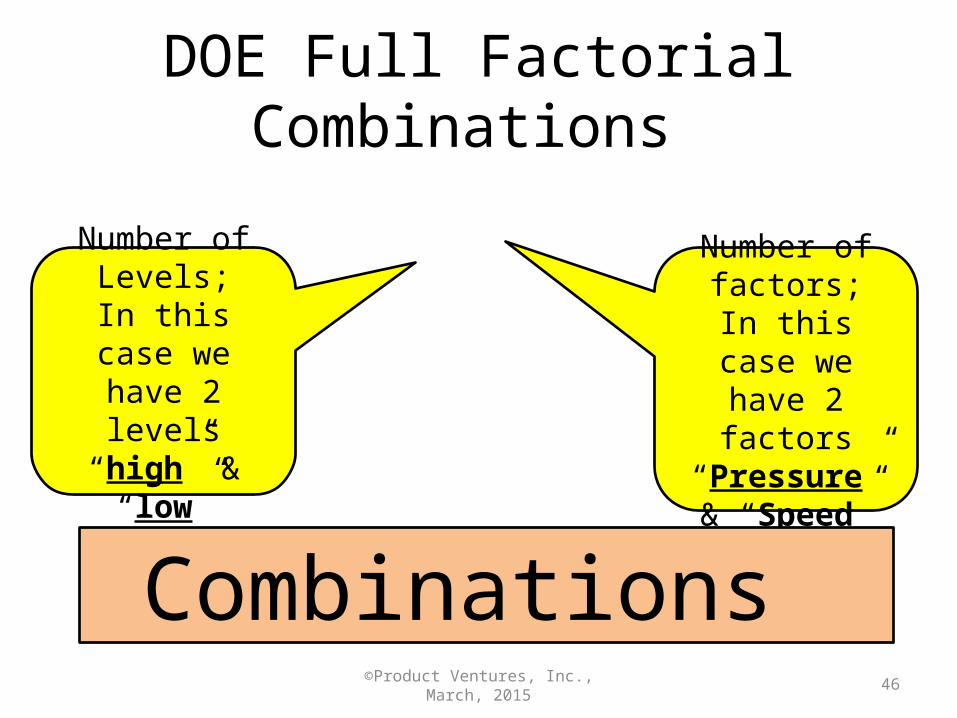
DOE Full Factorial Combinations
Number of factors;
In this case we have 2 factors “Pressure” &
“Speed”
Number of Levels;
In this case we have 2 levels
“high” & “low”
Combinations
©Product Ventures, Inc., March, 2015
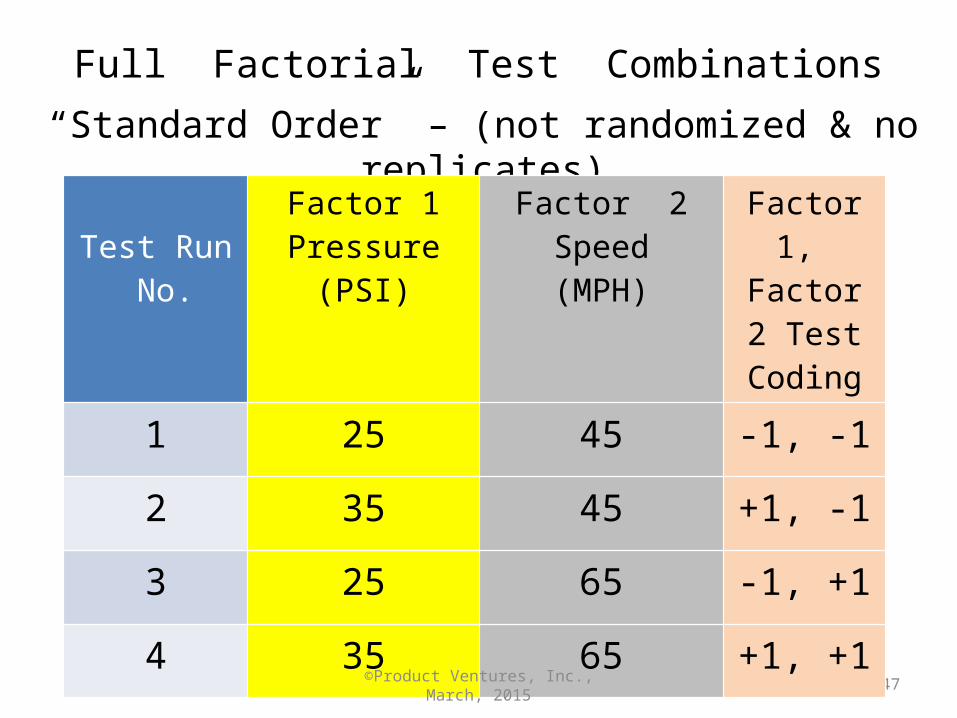
Full Factorial Test Combinations“Standard Order” – (not randomized & no replicates)
47
Test Run No.
Factor 1 Pressure (PSI)
Factor 2Speed(MPH)
Factor 1, Factor 2
Test Coding
1 25 45 -1, -1
2 35 45 +1, -1
3 25 65 -1, +1
4 35 65 +1, +1
©Product Ventures, Inc., March, 2015 48
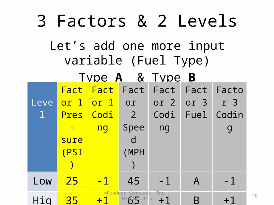
3 Factors & 2 LevelsLet’s add one more input variable (Fuel Type)
Type A & Type B
LevelFactor
1 Pres-sure (PSI)
Factor 1
Coding
Factor 2
Speed(MPH)
Factor 2
Coding
Factor 3
Fuel
Factor 3
Coding
Low 25 -1 45 -1 A -1
High 35 +1 65 +1 B +1
©Product Ventures, Inc., March, 2015 49
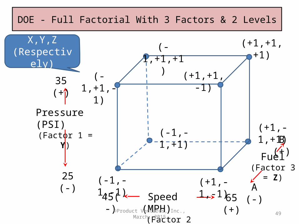
DOE - Full Factorial With 3 Factors & 2 Levels
Pressure (PSI)(Factor 1 = Y)
25 (-)
35 (+)
Speed (MPH)(Factor 2 = X)
45(-) 65 (+)
(-1,+1,-1)
(+1,+1,+1)
(-1,-1,-1) (+1,-1,-1)
Fuel (Factor 3 = Z)
A (-)
B (+)(+1,-1,+1)(-1,-1,+1)
(+1,+1,-1)
(-1,+1,+1)X,Y,Z (Respectively)
©Product Ventures, Inc., March, 2015 50
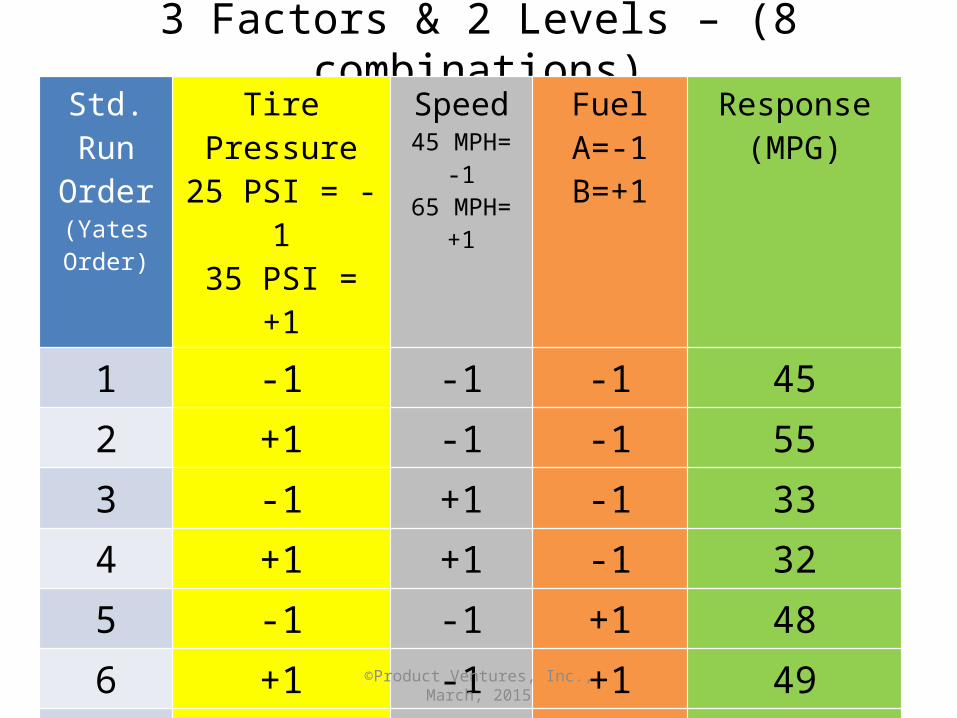
3 Factors & 2 Levels – (8 combinations)Std. Run Order
(Yates Order)
Tire Pressure25 PSI = -135 PSI = +1
Speed45 MPH= -165 MPH= +1
FuelA=-1B=+1
Response(MPG)
1 -1 -1 -1 45
2 +1 -1 -1 553 -1 +1 -1 334 +1 +1 -1 325 -1 -1 +1 486 +1 -1 +1 497 -1 +1 +1 258 +1 +1 +1 33
©Product Ventures, Inc., March, 2015 51
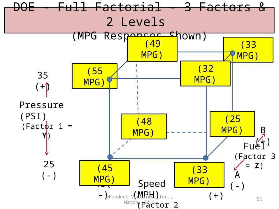
DOE - Full Factorial - 3 Factors & 2 Levels (MPG Responses Shown)
Pressure (PSI)(Factor 1 = Y)
25 (-)
35 (+)
Speed (MPH)(Factor 2 = X)
45(-) 65 (+)
(55 MPG)
(33 MPG)
(45 MPG) (33 MPG)
Fuel (Factor 3 = Z)
A (-)
B (+)(25 MPG)(48 MPG)
(32 MPG)
(49 MPG)
©Product Ventures, Inc., March, 2015 52
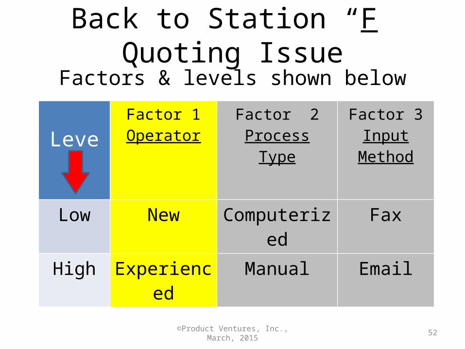
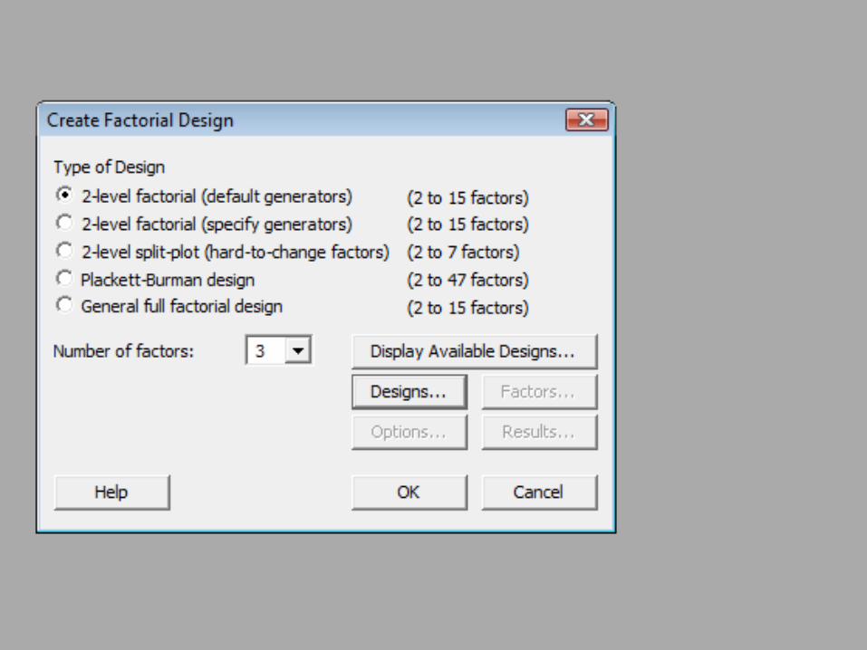
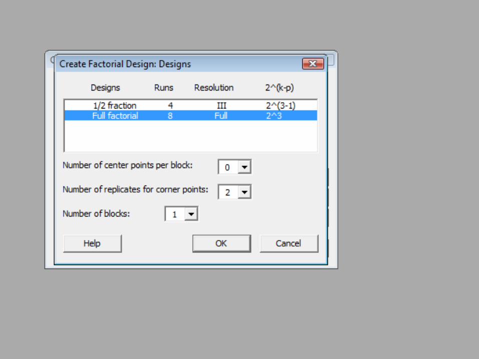
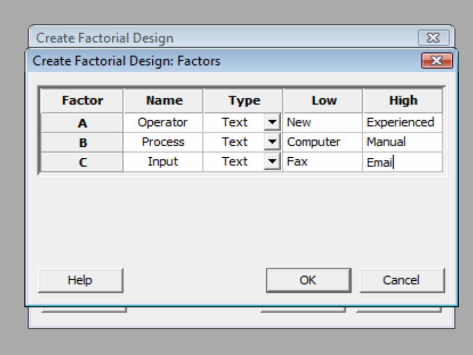
Back to Station “F” Quoting IssueFactors & levels shown below
LevelFactor 1 Operator
Factor 2Process
Type
Factor 3Input
Method
Low New Computerized Fax
High Experienced Manual Email
©Product Ventures, Inc., March, 2015 53
©Product Ventures, Inc., March, 2015 54
©Product Ventures, Inc., March, 2015 55
©Product Ventures, Inc., March, 2015 56
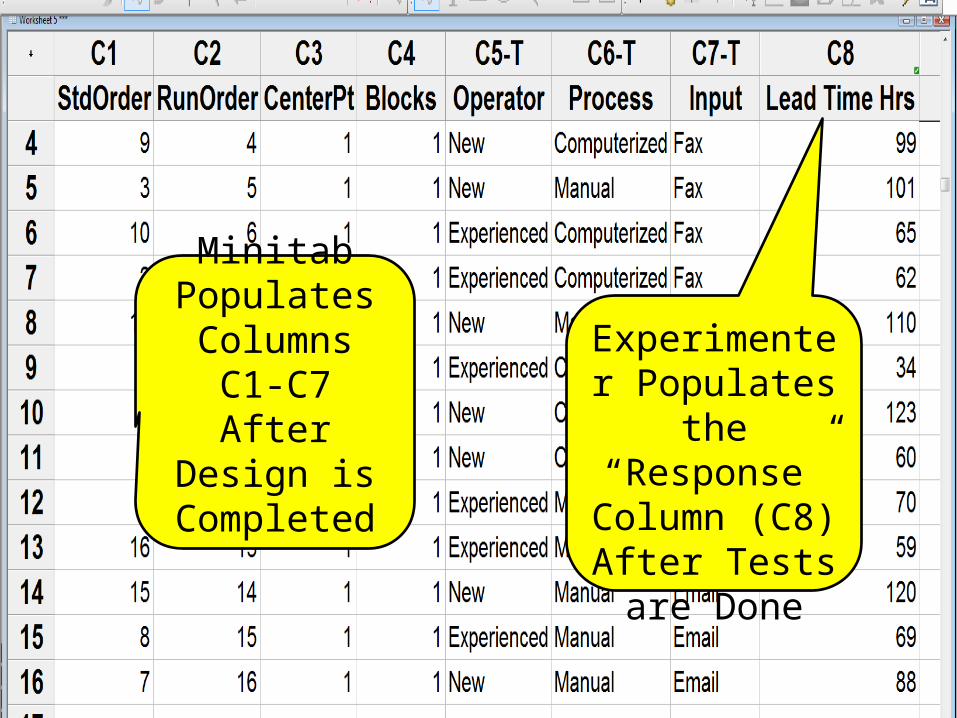
Minitab Populates
Columns C1-C7After Design is
Completed
Experimenter Populates the “Response” Column (C8)
After Tests are Done
©Product Ventures, Inc., March, 2015 57
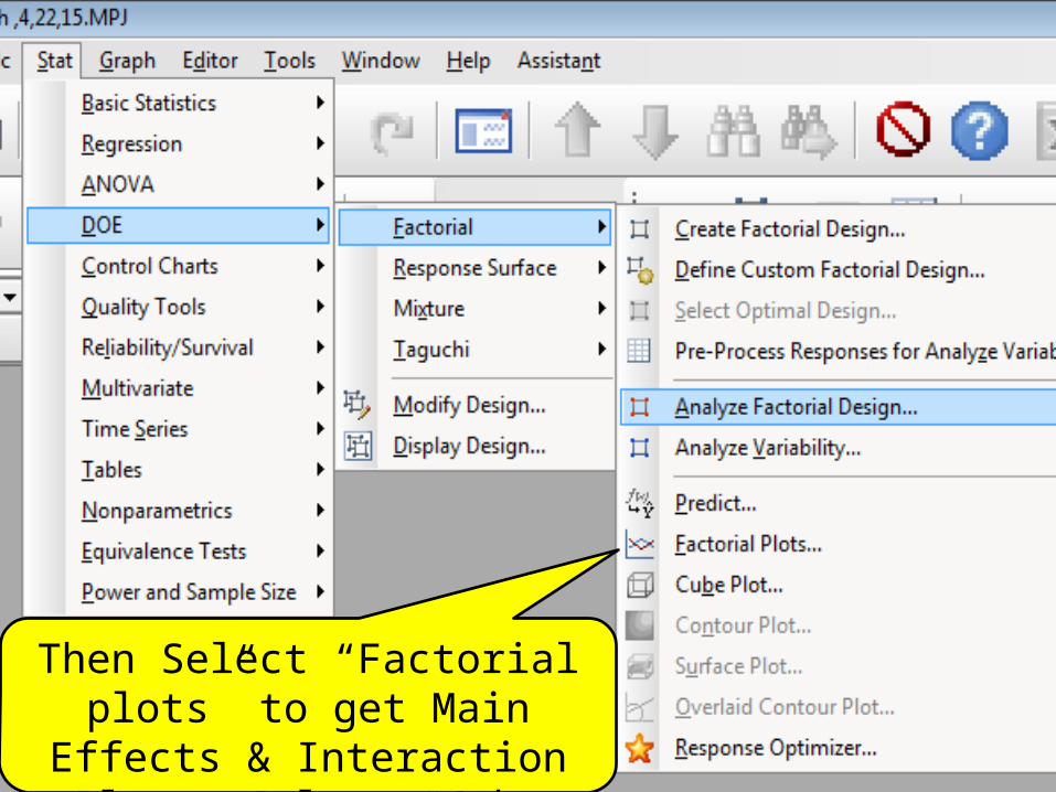
Then Select “Factorial plots” to get Main Effects & Interaction Plots. Select “Cube Plot” to Get Same.
©Product Ventures, Inc., March, 2015 58
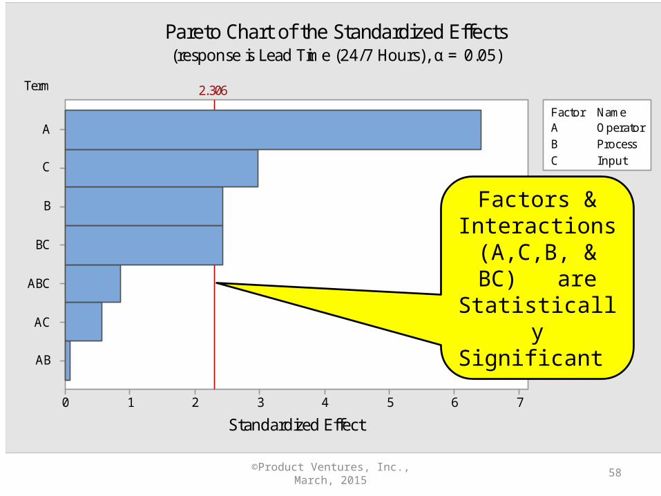
Term
AB
AC
ABC
BC
B
C
A
76543210
A OperatorB ProcessC Input
Factor Name
Standardized Effect
2.306
Pareto Chart of the Standardized Effects(response is Lead Time (24/7 Hours), α = 0.05)
Factors & Interactions
(A,C,B, & BC) are Statistically Significant
©Product Ventures, Inc., March, 2015 59
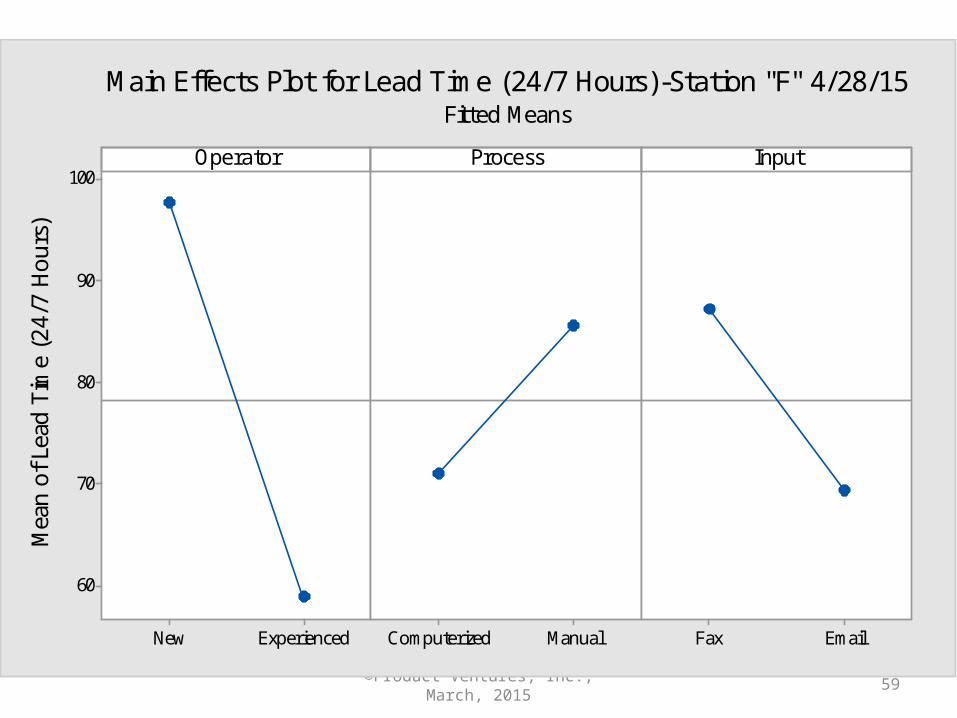
ExperiencedNew
100
90
80
70
60
ManualComputerized EmailFax
Operator
Mea
n of
Lea
d Ti
me
(24/
7 H
ours
)
Process Input
Main Effects Plot for Lead Time (24/7 Hours)-Station "F" 4/28/15Fitted Means
©Product Ventures, Inc., March, 2015 60
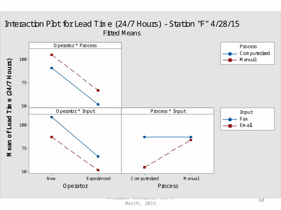
100
75
50
ExperiencedNew
100
75
50
ManualComputerized
Operator * Process
Operator * Input
Operator
Process * Input
Process
ComputerizedManual
Process
FaxEmail
Input
Mea
n o
f Le
ad T
ime
(24/
7 H
ours
)
Interaction Plot for Lead Time (24/7 Hours) - Station "F" 4/28/15Fitted Means
©Product Ventures, Inc., March, 2015 61
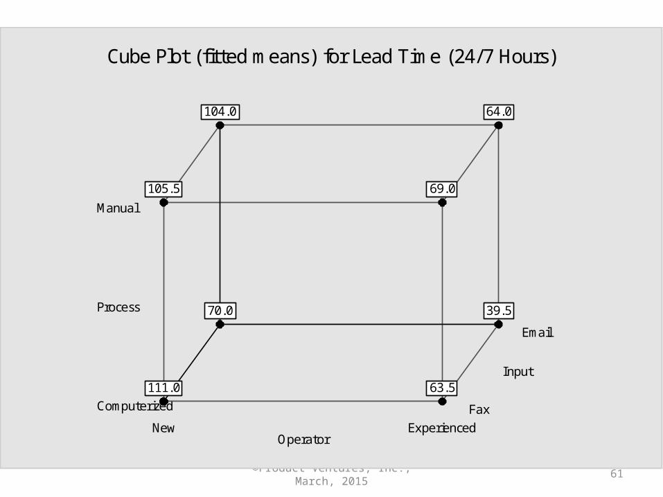
Fax
Manual
Computerized
ExperiencedNew
Input
Process
Operator
64.0
39.570.0
104.0
69.0
63.5111.0
105.5
Cube Plot (fitted means) for Lead Time (24/7 Hours)
©Product Ventures, Inc., March, 2015 62
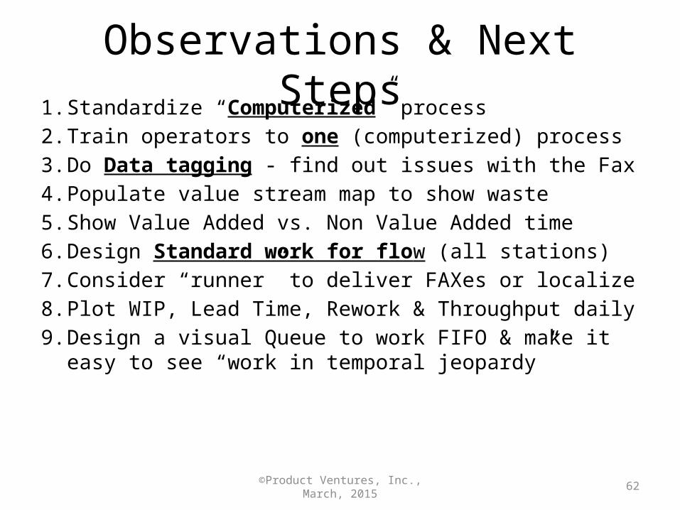
Observations & Next Steps1. Standardize “Computerized” process2. Train operators to one (computerized) process3. Do Data tagging - find out issues with the Fax4. Populate value stream map to show waste5. Show Value Added vs. Non Value Added time 6. Design Standard work for flow (all stations)7. Consider “runner” to deliver FAXes or localize8. Plot WIP, Lead Time, Rework & Throughput daily 9. Design a visual Queue to work FIFO & make it easy
to see “work in temporal jeopardy”
©Product Ventures, Inc., March, 2015 63
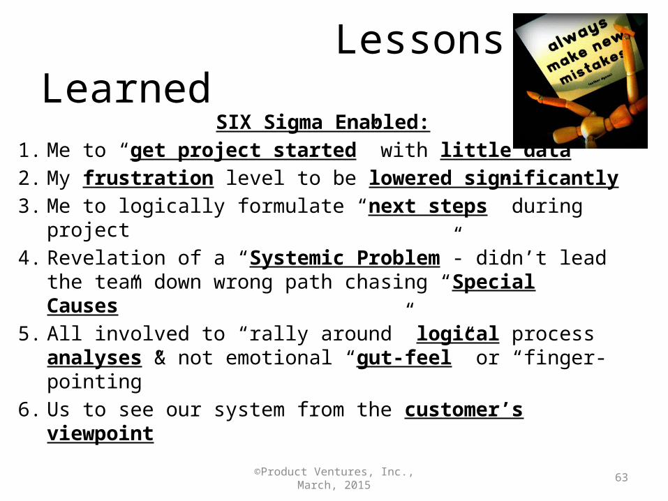
Lessons LearnedSIX Sigma Enabled:
1. Me to “get project started” with little data2. My frustration level to be lowered significantly3. Me to logically formulate “next steps” during project4. Revelation of a “Systemic Problem”- didn’t lead the
team down wrong path chasing “Special Causes” 5. All involved to “rally around” logical process analyses
& not emotional “gut-feel” or “finger-pointing”6. Us to see our system from the customer’s viewpoint