Wing kinematics measurement and aerodynamics of hovering droneflies.pdf

2014

INTRODUCTIONTo understand the aerodynamics, energetics and control of insect

flight, it is necessary to know the time history of the aerodynamic

forces and moments produced by the flapping wings. It is difficult,

even impossible, to directly measure the forces and moments on

the wings of a freely flying insect. Existing means of circumventing

this limitation are to measure experimentally or to compute

numerically the forces and moments on model insect wings (e.g.

Dickinson et al., 1999; Usherwood and Ellington, 2002a; Usherwood

and Ellington, 2002b; Sun and Tang, 2002a).

In order to use the experimental and computational methods to

obtain the aerodynamic forces and moments and to study insect

flight, measurements of wing kinematics and some morphological

parameters are required. Other researchers have measured wing

kinematics of many insects in free flight, using high-speed cine or

video; and also measured morphological data of these insects

(Ellington, 1984a; Ellington, 1984b; Dudley and Ellington, 1990;

Willmott and Ellington, 1997). But since these reported studies used

only one camera, the continuous time variation of wing orientation

(geometrical angle of attack, wing rotation rate, etc.) could not be

obtained. Recently, the time course of three-dimensional (3D) wing

motion of freely flying fruit flies was measured using three

orthogonally aligned, high-speed cameras (Fry et al., 2005).

Measurements of 3D wing motion of other insects are of great

interest, but some limitations to Fry et al.’s work meant that

morphological parameters such as weight and position of center of

mass could not be measured. If these data were also measured, one

could use them to test the experimental and computational models

(a reasonable test of the experimental and computational models is

that the measured or computed vertical force approximately balances

the insect weight and, in hovering flight, the horizontal force and

the pitching moment about the centre of mass of the insect are

approximately zero).

In the present study, we measure the time course of 3D wing

motion of hovering droneflies using three orthogonally alined high-

speed cameras and also measure the required morphological data,

and then employ the method of computational fluid dynamics (CFD)

to compute the aerodynamic forces and moments of the wings

flapping with the measured kinematics. The reasons we chose

droneflies are (1) droneflies might have different wing kinematics

from that of fruit flies used in Fry et al.’s study, (2) they are capable

of motionless hovering, and (3) they fly even in strongly lit

laboratory conditions. Comparison between computed results and

the conditions of vertical force being equal to weight, horizontal

force being equal to zero, and moment about the center of mass

being equal to zero, can provide a test of the computational model.

Analyzing the time courses of the wing motion and aerodynamic

forces and moments could provide insights into how the

aerodynamic forces and moments are produced and how the flight

balance is achieved. Using the computed results, the power

requirements can be readily estimated and the aerodynamic

efficiency of flight examined.

MATERIALS AND METHODSAnimals

We netted droneflies of the species Eristalis tenax Linnaeus in a

suburb of Beijing in September 2006. All experiments were

The Journal of Experimental Biology 211, 2014-2025Published by The Company of Biologists 2008doi:10.1242/jeb.016931

Wing kinematics measurement and aerodynamics of hovering droneflies

Yanpeng Liu* and Mao SunInstitute of Fluid Mechanics, Beijing University of Aeronautics and Astronautics, Beijing 100083, People’s Republic of China

*Author for correspondence (e-mail: [email protected])

Accepted 9 April 2008

SUMMARYThe time courses of wing and body kinematics of three freely hovering droneflies (Eristalis tenax) were measured using 3D high-speed video, and the morphological parameters of the wings and body of the insects were also measured. The measured wingkinematics was used in a Navier–Stokes solver to compute the aerodynamic forces and moments acting on the insects. The timecourses of the geometrical angle of attack and the deviation angle of the wing are considerably different from that of fruit fliesrecently measured using the same approach. The angle of attack is approximately constant in the mid portions of a half-stroke (adownstroke or upstroke) and varies rapidly during the stroke reversal. The deviation angle is relatively small and is higher at thebeginning and the end of a half-stroke and lower at the middle of the half-stroke, giving a shallow U-shaped wing-tip trajectory.For all three insects considered, the computed vertical force is approximately equal to the insect weight (the difference is lessthan 6% of the weight) and the computed horizontal force and pitching moment about the center of mass of the insect areapproximately zero. The computed results satisfying the equilibrium flight conditions, especially the moment balance condition,validate the computation model. The lift principle is mainly used to produce the weight-supporting vertical force, unlike the fruitflies who use both lift and drag principles to generate the vertical force; the vertical force is mainly due to the delayed stallmechanism. The magnitude of the inertia power is larger than that of the aerodynamic power, and the largest possible effect ofelastic storage amounts to a reduction of flight power by around 40%, much larger than in the case of the fruit fly.

Supplementary material available online at http://jeb.biologists.org/cgi/content/full/211/13/2014/DC1

Key words: dronefly, hovering, wing kinematics measurement, aerodynamics, Navier–Stokes simulation.

THE JOURNAL OF EXPERIMENTAL BIOLOGY

2015Aerodynamics of hovering droneflies

conducted in the same day of capture. Only the most vigorous

individuals were selected for filming.

3D high-speed filmWe filmed the hovering flight of the droneflies in an enclosed flight

chamber using three orthogonally aligned synchronized high-speed

cameras (MotionXtra HG-LE, 5000framess–1, shutter speed 50μs,

resolution 512�320 pixels). The flight chamber, a cube of

15�15�15cm3, was built from translucent glass. We backlit each

camera view using densely packed arrays of light emitting diodes

(LED) covered with diffusion paper. The reason we used LED arrays

as the light source was that they produced much less heat than cine

lights at the elevated light levels required for high-speed filming.

The filming was started only when the insect hovered in the cubic

zone of approximately 5�5�5cm3 at the central region of the

chamber, which represented the intersecting field of views of the

the three cameras.

Measurement of wing and body kinematicsUsing a flat calibration panel to calibrate the cameras, one can obtain

the transform matrices between the world coordinate system and

three image coordinate systems, which are called projection matrices.

Based on the basic principles of stereo vision, the projections of the

scene point in the world coordinate system onto any image

coordinate system can be calculated, provided that the point’s

coordinate in the world coordinate system and projection matrices

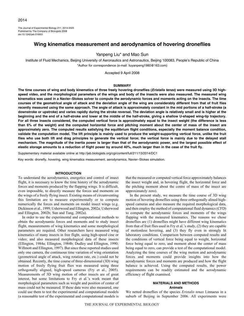
are known. The general structure of a trinocular stereo vision system

is shown in Fig.1.

Let (Xw Yw Zw) be the world coordinate system; let (XC1 YC1

ZC1), (XC2 YC2 ZC2) and (XC3 YC3 ZC3) be the camera coordinate

systems of camera 1, 2 and 3, respectively; let (u1 v1), (u2 v2) and

(u3 v3) be the image coordinate systems of cameras 1, 2 and 3,

respectively. Let P be an arbitrary point, whose coordinates are

Xw, Yw and Zw in the world frame, XC1, YC1 and ZC1 in the frame

of camera 1, XC2, YC2 and ZC2 in the frame of camera 2, XC3, YC3

and ZC3 in the frame of camera 3. Let p1, p2 and p3 be the projective

points of P on the three cameras; p1’s coordinates in the image

frame of camera 1 are u1 and v1; p2’s coordinates in the image

frame of camera 2 are u2 and v2; p3’s coordinates in the image

frame of camera 3 are u3 and v3. The coordinate transformation

between the world coordinate system and the three image coordinate

systems are:

where M1, M2 and M3 are projection matrices of camera 1, camera

2 and camera 3, respectively. Let m1i,j, m2i,j and m3i,j (i, j=1,2,3)

denote the elements of M1, M2 and M3, respectively. Eliminating

ZC1, ZC2 and ZC3 from Eqn1 gives:

⎧

⎨

⎩

⎢

⎢. (4)

m311 Xw + m312Yw + m313 Zw + m314

− u3 Xw m331 − u3Yw m332 − u3Zw m333 = u3

m321 Xw + m322Yw + m323 Zw + m324

− v3 Xw m331 − v3Yw m332 − v3Zw m333 = v3

, (3)

⎧

⎨

⎩

⎢

⎢

m211 Xw + m212Yw + m213 Zw + m214

− u2 Xw m231 − u2Yw m232 − u2Zw m233 = u2

m221 Xw + m222Yw + m223 Zw + m224

− v2 Xw m231 − v2Yw m232 − v2Zw m233 = v2

, (1)

Zc1

u1

v1

1

⎡

⎣

⎢⎢⎢

⎤

⎦

⎥⎥⎥

= M1

Xw

Yw

Zw

1

⎡

⎣

⎢⎢⎢⎢⎢

⎤

⎦

⎥⎥⎥⎥⎥

,

Zc2

u2

v2

1

⎡

⎣

⎢⎢⎢

⎤

⎦

⎥⎥⎥

= M2

Xw

Yw

Zw

1

⎡

⎣

⎢⎢⎢⎢⎢

⎤

⎦

⎥⎥⎥⎥⎥

,

Zc3

u3

v3

1

⎡

⎣

⎢⎢⎢

⎤

⎦

⎥⎥⎥

= M3

Xw

Yw

Zw

1

⎡

⎣

⎢⎢⎢⎢⎢

⎤

⎦

⎥⎥⎥⎥⎥

, (2)

m111 Xw + m112Yw + m113 Zw + m114

− u1 Xw m131 − u1Yw m132 − u1Zw m133 = u1

m121 Xw + m122Yw + m123 Zw + m124

− v1Xw m131 − v1Yw m132 − v1Zw m133 = v1

⎧

⎨

⎩

⎢

⎢

C1X

C1YC1Z

1f

1v

1u

1p

P

X

WY

WO

WZ

2u

2v

2f

3p

C2ZC2X

C2Y

3u3v

2p3f

C3Z

C3YC3X

W

Fig. 1. Model of trinocular stereo vision system. (XW YW ZW), theworld coordinate system; (XC1 YC1 ZC1), (XC2 YC2 ZC2) and (XC3

YC3 ZC3), the camera coordinate systems of cameras 1, 2 and 3,respectively; (u1 v1), (u2 v2) and (u3 v3), image coordinate systemsof camera 1, 2 and 3, respectively. P, an arbitrary point; p1, p2 andp3, the projective points and f1, f2 and f3, the focal length ofcameras 1, 2 and 3, respectively.


2016

The coordinates of point P’s projection onto all three image

coordinate systems can be determined via Eqn2–4.

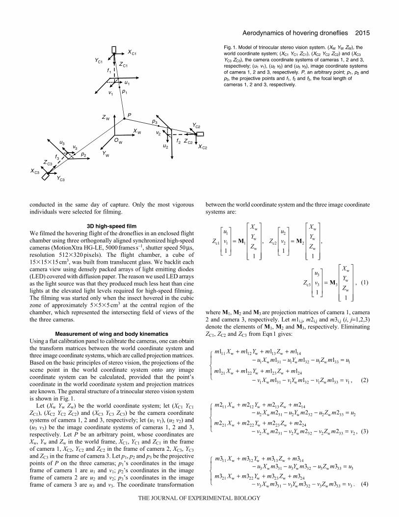
We take a line segment, whose length is equal to the body length

of the insect, to represent the body of the insect, and used the outline

of the wing obtained from scanned picture of the wing (see Fig.2A)

to represent the wing. The line segment of the body and the outline

of a wing are designated as the models of the body and the wing,

respectively. They can be represented as a set of points. Using the

method described above, we can easily computed the projection of

the point set on all the three image coordinate systems.

We developed a toolbox for Matlab (The MathWorks, Inc.,

Natick, MA, USA) to extract the position and attitude of the body

and of the wings from images captured by all three cameras. We

put the models of the body and the wings into the world coordinate

system, then changed the positions and attitudes of those models

until the best overlap between a model’s projection and displayed

frame was achieved in all three views. At this point, the positions

and attitudes of those models would be taken as the positions and

attitudes of the body and wings of the insect. Generally, several

Y. Liu and M. Sun

readjustments of each model’s position and attitude were required

to obtain a satisfactory overlap.

Measurement of morphological parametersThe present method of measuring the morphological parameters

follows, for the most part, the detailed description of the method

given by Ellington (Ellington, 1984a).

The insect was killed with ethyl acetate vapor after filming. The

total mass m was measured to an accuracy of ±0.01mg. The wings

were then cut from the body and the mass of the wingless body

measured. The wing mass mwg was determined from the difference

between the total mass and the mass of wingless body.

Immediately after cutting the wings from the body, the shape of

one of them was scanned using a scanner (HP scanjet 4370;

resolution 3600�3600 d.p.i.). A sample of the scanned picture of

a wing is shown in Fig.2A. Using the scanned picture, wing length

R (the distance between the wing base and the wing tip) (see

Ellington, 1984a) and local wing chord length were measured to an

accuracy better than ±0.5%. Parameters including wing area, mean

Fig. 2. (A) Wing model. (B) Example of framesrecorded by the three cameras. See text for details.

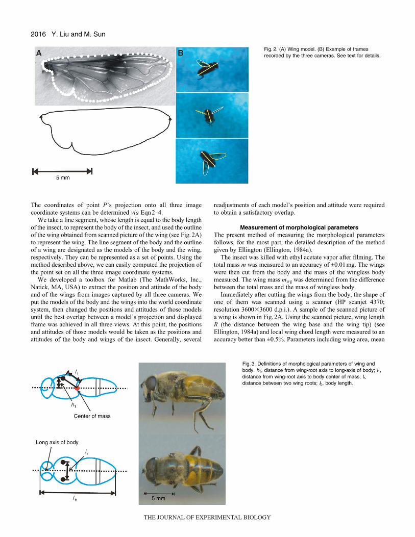
Fig. 3. Definitions of morphological parameters of wing andbody. h1, distance from wing-root axis to long-axis of body; l1,distance from wing-root axis to body center of mass; lr,distance between two wing roots; lb, body length.



chord length, radius of second moment of wing area, etc., were

computed using the measured wing shape.

The wingless body (with legs removed) was scanned from two

perpendicular directions (the dorsoventral and lateral views;

Fig. 3). Following Ellington (Ellington, 1984a), the cross section

of the body was taken as ellipse and a uniform density was assumed

for the body. With these assumptions and the measured body shape,

the center of mass of body could be determined. Body length (lb)

and distance between the wing roots (lr) were measured from the

dorsal views; distance between the wing-base axis and the center

of mass (l1) and distance between the wing-base axis and the long

axis of the body (h1) were measured from the lateral view (the

pitch moment of inertia about the center of mass could also be

determined).

Computation of aerodynamic forces and moments and powerrequirements

The aerodynamic forces and moments were computed using the CFD

method. On the basis of studies on wing–wing interactions

(Lehmann et al., 2005; Sun and Yu, 2006), aerodynamic interactions

between the left and right wings could be neglected. During

hovering flight, the body did not move, and it was assumed that the

aerodynamic interaction between the body and the wings was

negligible. Therefore in the present CFD model, the body was

neglected and only the flows around one wing were computed (the

aerodynamic force and moment produced by the other wing were

derived from the results of the computed wing). The wing planform

of the insect was obtained from the present measured data. The wing

section was assumed to be a flat plate with rounded leading and

trailing edges, the thickness of which was 3% of the mean chord

length of the wing.

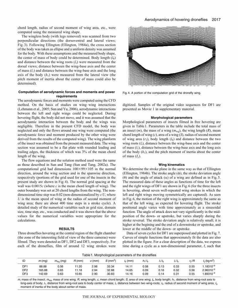
The flow equations and the solution method used were the same

as those described in Sun and Tang (Sun and Tang, 2002a). The

computational grid had dimensions 100�99�105 in the normal

direction, around the wing section and in the spanwise direction,

respectively (portions of the grid used for one of the insects in the

present study are shown in Fig.4). The normal grid spacing at the

wall was 0.0015c (where c is the mean chord length of wing). The

outer boundary was set at 20 chord lengths from the wing. The non-

dimensional time step was 0.02 (non-dimensionalized by c/U, where

U is the mean speed of wing at the radius of second moment of

wing area; there are about 400 time steps in a stroke cycle). A

detailed study of the numerical variables such as grid size, domain

size, time step, etc., was conducted and it was shown that the above

values for the numerical variables were appropriate for the

calculations.

RESULTSThree droneflies hovering at the central region of the flight chamber

(the zone of the interesting field of view of the three cameras) were

filmed. They were denoted as DF1, DF2 and DF3, respectively. For

each of the droneflies, film of around 12 wing strokes were

digitized. Samples of the original video sequences for DF1 are

presented as Movie 1 in supplementary material.

Morphological parametersMorphological parameters of insects filmed in free hovering are

given in Table1. Parameters in the table include the total mass of

an insect (m), the mass of a wing (mwg), the wing length (R), mean

chord length of wing (c), area of a wing (S), radius of second moment

of wing area (r2), body length (lb) and distance between the two

wing roots (lr), distance between the wing-base axis and the center

of mass (l1), distance between the wing-base axis and the long axis

of the body (h1), and the pitch moment of inertia about the center

of mass (Iy).

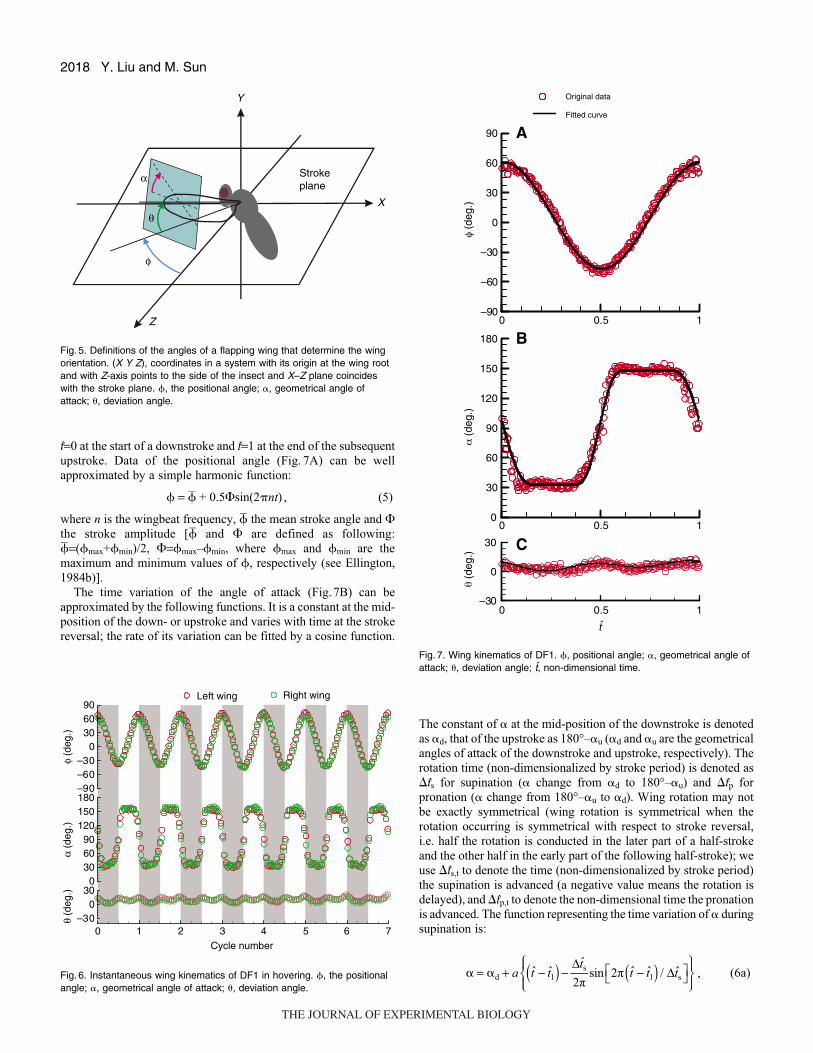
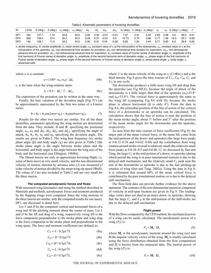
Wing kinematicsWe determine the stroke plane in the same way as that of Ellington

(Ellington, 1984b). The stroke angle (�), the stroke deviation angle

(�) and the angle of attack (�) of a wing are defined as in Fig.5.

The measured data of these angles as functions of time for the left

and the right wings of DF1 are shown in Fig.6 (for the three insects

in hovering, about seven well-repeated wing strokes in which the

left and right wings moving symmetrically are captured). As seen

in Fig.6, the motion of the right wing is approximately the same as

that of the left wing, as expected for hovering flight. The stroke

positional angle varies with time approximately as a sinusoidal

function. The angle of attack does not vary significantly in the mid-

position of the down- or upstroke, but varies sharply during the

stroke reversal. The stroke deviation angle is relatively small; it is

higher at the begining and the end of a downstroke or upstroke, and

lower at the middle of the down- or upstroke.

Data of seven cycles for DF1 are superposed and plotted in Fig.7.

Curves of simple functions that approximately fit the data are also

plotted in the figure. For a clear description of the data, we express

time during a cycle as a non-dimensional parameter, t, such that

Fig. 4. A portion of the computation grid of the dronefly wing.

Table1. Morphological parameters of the droneflies

ID m (mg) mwg (mg) R (mm) c (mm) S (mm2) lb (mm) h1/lb l1/lb lr /lb r2 /R Iy (kg m2)

DF1 88.88 0.56 11.20 2.98 33.34 14.11 0.08 0.13 0.33 0.55 1.18310–9

DF2 165.88 0.65 11.18 2.94 32.88 14.65 0.09 0.16 0.32 0.56 2.96310–9

DF3 142.69 0.63 10.65 2.90 30.83 14.16 0.09 0.14 0.31 0.55 1.89310–9

m, mass of the insect; mwg, mass of one wing; R, wing length; c, mean chord length; S, area of one wing; lb, body length; h1, distance from wing-root axis tolong-axis of body; l1, distance from wing-root axis to body center of mass; lr, distance between two wing-roots; r2, radius of second moment of wing area; Iy,moment of inertia of the body about center of mass.


2018

t=0 at the start of a downstroke and t=1 at the end of the subsequent

upstroke. Data of the positional angle (Fig. 7A) can be well

approximated by a simple harmonic function:

� = � + 0.5�sin(2�nt) , (5)

where n is the wingbeat frequency, � the mean stroke angle and �the stroke amplitude [� and � are defined as following:

�=(�max+�min)/2, �=�max–�min, where �max and �min are the

maximum and minimum values of �, respectively (see Ellington,

1984b)].

The time variation of the angle of attack (Fig.7B) can be

approximated by the following functions. It is a constant at the mid-

position of the down- or upstroke and varies with time at the stroke

reversal; the rate of its variation can be fitted by a cosine function.

Y. Liu and M. Sun

The constant of � at the mid-position of the downstroke is denoted

as �d, that of the upstroke as 180°–�u (�d and �u are the geometrical

angles of attack of the downstroke and upstroke, respectively). The

rotation time (non-dimensionalized by stroke period) is denoted as

�ts for supination (� change from �d to 180°–�u) and �tp for

pronation (� change from 180°–�u to �d). Wing rotation may not

be exactly symmetrical (wing rotation is symmetrical when the

rotation occurring is symmetrical with respect to stroke reversal,

i.e. half the rotation is conducted in the later part of a half-stroke

and the other half in the early part of the following half-stroke); we

use �ts,t to denote the time (non-dimensionalized by stroke period)

the supination is advanced (a negative value means the rotation is

delayed), and �tp,t to denote the non-dimensional time the pronation

is advanced. The function representing the time variation of � during

supination is:

, (6a)

= d + a t̂ − t̂1( ) −Δt̂s

2πsin 2π t̂ − t̂1( ) / Δt̂s⎡⎣ ⎤⎦

⎧⎨⎪

⎩⎪

⎫⎬⎪

⎭⎪� �

Strokeplane

X

Y

Z

φ

α

θ

Fig. 5. Definitions of the angles of a flapping wing that determine the wingorientation. (X Y Z), coordinates in a system with its origin at the wing rootand with Z-axis points to the side of the insect and X–Z plane coincideswith the stroke plane. �, the positional angle; �, geometrical angle ofattack; �, deviation angle.

–90–60–30

0306090

0306090

120150180

0 1 2 3 4 5 6 7–30

030

Left wing Right wing

Cycle number

φ (d

eg.)

α (d

eg.)

θ (d

eg.)

Fig. 6. Instantaneous wing kinematics of DF1 in hovering. �, the positionalangle; �, geometrical angle of attack; �, deviation angle.

0 0.5

t

1

0 0.5 1

Original data

Fitted curve

0 0.5 1–90

–60

–30

0

30

60

90 A

φ (d

eg.)

α (

deg.

)θ

(deg

.)

0

30

60

90

120

150

180 B

C

–30

0

30

Fig. 7. Wing kinematics of DF1. �, positional angle; �, geometrical angle ofattack; �, deviation angle; t, non-dimensional time.



where a is a constant:

a = (180°–�u–�d) / �ts . (6b)

t1 is the time when the wing-rotation starts:

t1 = 0.5 – �ts / 2 – �ts,t . (6c)

The expression of the pronation can be written in the same way.

Finally, the time variation of the deviation angle (Fig.7C) can

be approximately represented by the first two terms of a Fourier

series:

� = �0 + �1sin(2�nt+1) + �2sin(4�nt+2) . (7)

Results for the other two insects are similar. For all the three

droneflies, parameters specifying the wing motion are determined

from the data. They include: � and �, specifying the positional

angle; �u, �d and �ts, �tp, �ts,t and �tp,t, specifying the angle of

attack; �0, �1, �2, 1 and 2, specifying the deviation angle. The

results are given in Table2. The wing beat frequency (n), stroke

plane angle () and body angle (�) are also given in Table2 [the

stroke plane angle is the angle between stroke plane and the

horizontal, and body angle is the angle between the long axis of the

body and the horizontal (see Ellington, 1984b)].

The filmed insects are only in approximate hovering flight; i.e.

some of them move at very small velocity, and the non-dimensional

velocity of motion, denoted by advance ratio (J) was measured (Jis the velocity of motion divided by the mean wing-tip speed 2�nR).

The values of J are also included in Table2 and are very small for

the three insects.

The computed aerodynamic forces and flowsWith measured wing kinematics and using the method described in

Materials and methods, aerodynamic forces and moments produced

by the flapping wings were computed. Since the wing motions of

the three insects are similar, only the computed results for one insect,

DF1, are discussed in detail here.

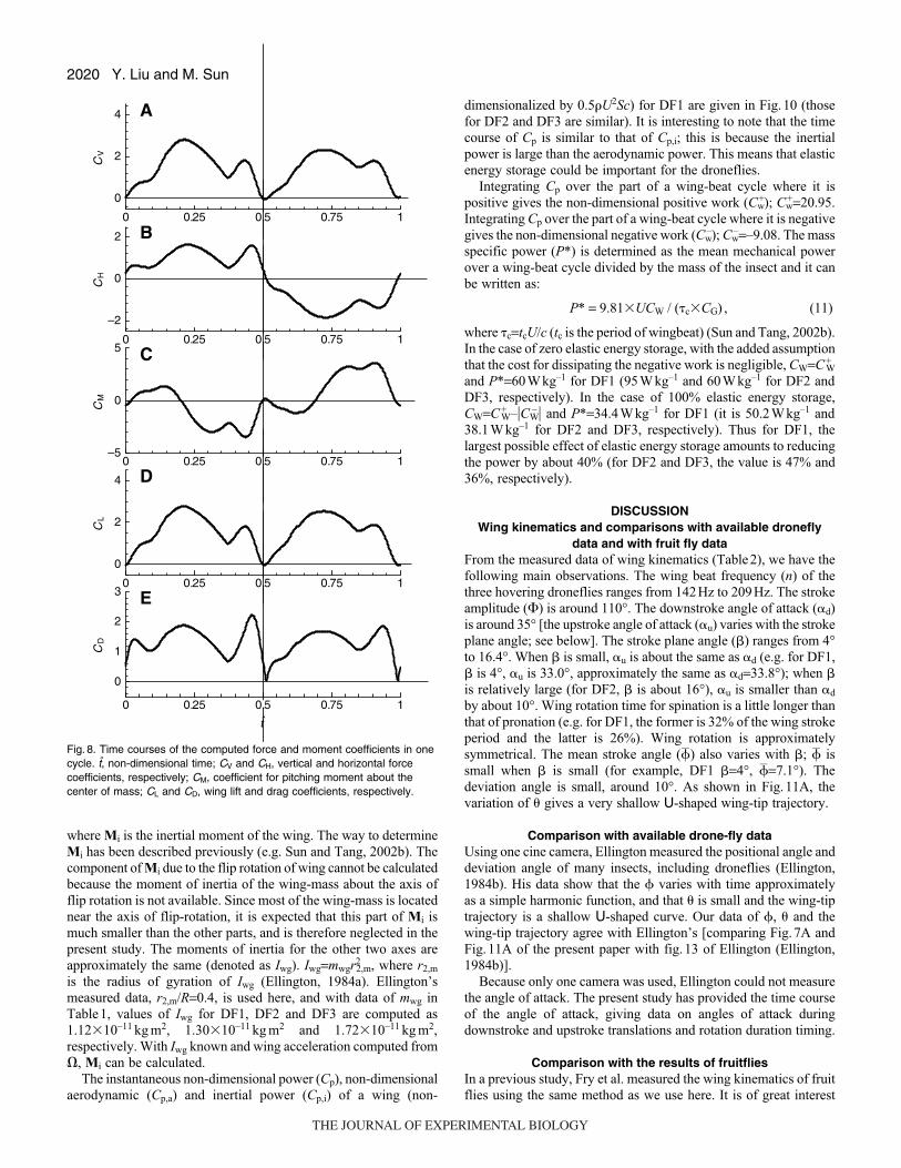
Let V and H be the computed vertical and horizontal forces of a

wing and M the pitching moment about the center of mass. Let Land D be the lift and drag of a wing, respectively (wing lift is the

force component perpendicular to the stroke plane and wing drag

is the force component in the stroke plane and perpendicular to the

wing span). The force and moment coefficients are defined as:

CV = V / 0.5�U2S (8a)

CH = H / 0.5�U2S (8b)

CM = M / 0.5�U2Sc (8c)

CL = L / 0.5�U2S (8d)

CD = D / 0.5�U2S , (8e)

where U is the mean velocity of the wing at r2 (U=�nr2) and � the

fluid density. Fig.8 gives the time courses of CV, CH, CM, CL and

CD in one cycle.

The downstroke produces a little more wing lift and drag than

the upstroke (see Fig. 8D,E), because the angle of attack of the

downstroke is a little larger than that of the upstroke (�d=33.8°

and �u=33.0°). The vertical force is approximately the same as

the wing lift (comparing Fig. 8A with D), because the stroke

plane is almost horizontal ( is only 4°). From the data in

Fig. 8A, the azimuthal position of the line of action of the vertical

force of a downstroke or an upstroke can be calculated. The

calculation shows that the line of action is near the position of

the mean stroke angle, about 3° before and 5° after the position

of the mean stroke angle for the downstroke and the upstroke,

respectively.

As seen from the time courses of force coefficients (Fig.8), the

major part of the mean vertical force, or the mean lift, come from

the mid-portions of the down- and upstrokes (the large force peaks

at t=0.12–0.38 and t=0.62–0.88) and the contribution from wing

rotation around stroke reversal is relatively small (the relatively small

force peaks at t=0.38–0.5 and t=0.88–1). As discussed by Sun and

Tang, the large CL in the mid-portion of a down- or upstroke (during

which period the wing is in pure translational motion) is due to the

delayed stall mechanism, and the relatively small CL peak near the

end of the downstroke or upstroke is due to the fast pitching-up

rotation of wing (Sun and Tang, 2002a). Using the data in Fig.8,

it is estimated that around 60% of the mean vertical force is

contributed by the pure translational motion, or is due to the delayed

stall mechanism.

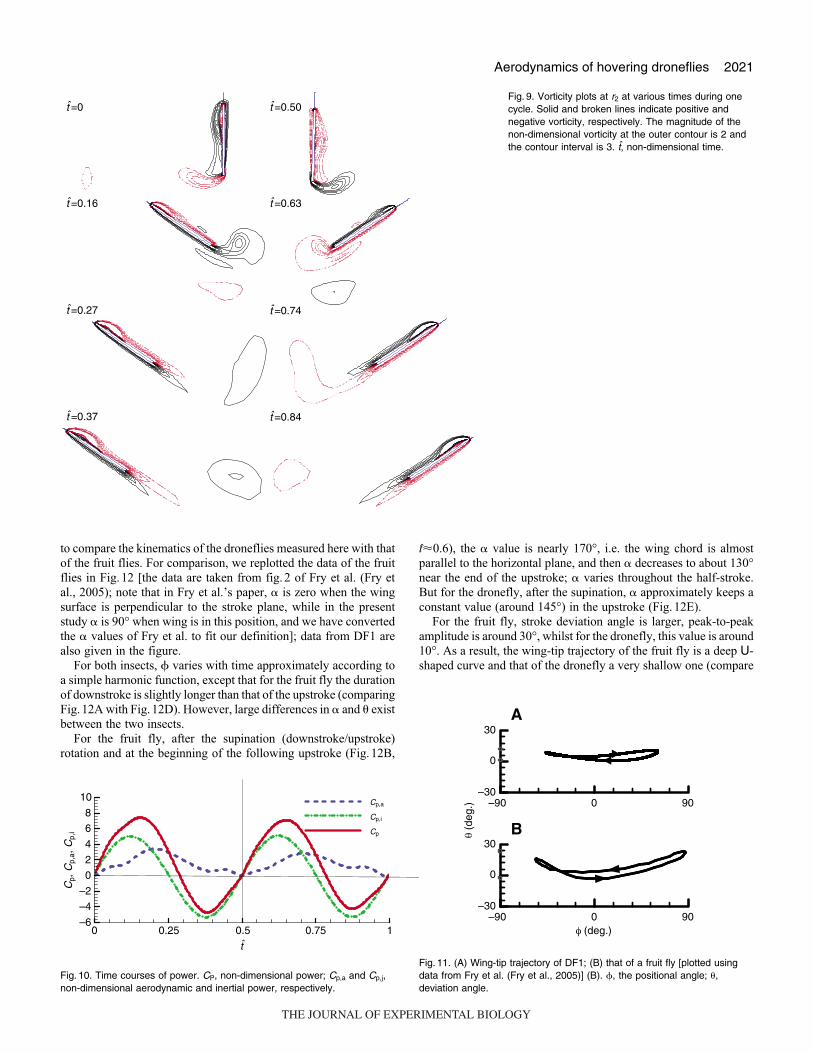
The flow-field data can provide further evidence for the above

statement. The contours of the non-dimensional spanwise component

of vorticity at mid-span location are given in Fig.9. The leading-

edge vortex does not shed in an entire down- or upstroke, showing

that the large CL and CD in the mid-portion of the half-stroke are

due to the delayed stall mechanism.

Flight powerWith the flows computed by the CFD method, the mechanical power

of a wing can be easily calculated. The aerodynamic power of a

wing (Pa) is:

Pa =Ma. , (9)

where Ma is the aerodynamic moment around the wing root and

the angular velocity vector of the wing. Ma is readily calculated

using the force distribution obtained from the flow computation

and is known from the measured data. The inertial power of

the wing (Pi) is:

Pi =Mi. , (10)

Table2. Kinematic parameters of hovering droneflies

ID n (Hz) � (deg.) � (deg.) �d (deg.) �u (deg.) �tp �ts �tp,t �ts,t �0 (deg.) �1 (deg.) �2 (deg.) 1 2 (deg.) � (deg.) J

DF1 164 107.1 7.12 33.8 33.0 0.26 0.32 –0.01 –0.01 7.07 2.31 3.44 2.83 2.08 4.0 38.0 0.01DF2 209 109.5 13.4 35.5 24.2 0.29 0.31 –0.01 0.0 10.73 2.75 3.96 2.77 1.56 16.4 29.7 0.00DF3 142 109.1 11.9 34.2 34.2 0.30 0.31 0.03 –0.02 6.82 1.55 3.44 0.71 0.83 6.2 39.8 0.02

n, stroke frequency; �, stroke amplitude; �, mean stroke angle; �d, constant value of � at the mid-position of the downstroke; �u, constant value of � at themid-position of the upstroke; �tp, non-dimensional time duration for pronation; �ts, non-dimensional time duration for supination; �tp,t, non-dimensionaladvance time for pronation; �ts,t, non-dimensional advance time for supination; �0, constant value of Fourier series of deviation angle; �1, amplitude of thefirst harmonic of Fourier series of deviation angle; �2, amplitude of the second harmonic term of deviation angle; 1, phase angle of the first harmonic ofFourier series of deviation angle; 2, phase angle of the second harmonic of Fourier series of deviation angle; , stroke plane angle; �, body angle; J,advanced ratio.


2020

where Mi is the inertial moment of the wing. The way to determine

Mi has been described previously (e.g. Sun and Tang, 2002b). The

component of Mi due to the flip rotation of wing cannot be calculated

because the moment of inertia of the wing-mass about the axis of

flip rotation is not available. Since most of the wing-mass is located

near the axis of flip-rotation, it is expected that this part of Mi is

much smaller than the other parts, and is therefore neglected in the

present study. The moments of inertia for the other two axes are

approximately the same (denoted as Iwg). Iwg=mwgr22,m, where r2,m

is the radius of gyration of Iwg (Ellington, 1984a). Ellington’s

measured data, r2,m/R=0.4, is used here, and with data of mwg in

Table1, values of Iwg for DF1, DF2 and DF3 are computed as

1.12�10–11 kg m2, 1.30�10–11 kg m2 and 1.72�10–11 kg m2,

respectively. With Iwg known and wing acceleration computed from

, Mi can be calculated.

The instantaneous non-dimensional power (Cp), non-dimensional

aerodynamic (Cp,a) and inertial power (Cp,i) of a wing (non-

Y. Liu and M. Sun

dimensionalized by 0.5�U2Sc) for DF1 are given in Fig.10 (those

for DF2 and DF3 are similar). It is interesting to note that the time

course of Cp is similar to that of Cp,i; this is because the inertial

power is large than the aerodynamic power. This means that elastic

energy storage could be important for the droneflies.

Integrating Cp over the part of a wing-beat cycle where it is

positive gives the non-dimensional positive work (Cw+); Cw

+=20.95.

Integrating Cp over the part of a wing-beat cycle where it is negative

gives the non-dimensional negative work (Cw–); Cw

–=–9.08. The mass

specific power (P*) is determined as the mean mechanical power

over a wing-beat cycle divided by the mass of the insect and it can

be written as:

P* = 9.81�UCW / (�c�CG) , (11)

where �c=tcU/c (tc is the period of wingbeat) (Sun and Tang, 2002b).

In the case of zero elastic energy storage, with the added assumption

that the cost for dissipating the negative work is negligible, CW=C+W

and P*=60Wkg–1 for DF1 (95Wkg–1 and 60Wkg–1 for DF2 and

DF3, respectively). In the case of 100% elastic energy storage,

CW=C+W–�CW

– � and P*=34.4Wkg–1 for DF1 (it is 50.2Wkg–1 and

38.1Wkg–1 for DF2 and DF3, respectively). Thus for DF1, the

largest possible effect of elastic energy storage amounts to reducing

the power by about 40% (for DF2 and DF3, the value is 47% and

36%, respectively).

DISCUSSIONWing kinematics and comparisons with available dronefly

data and with fruit fly dataFrom the measured data of wing kinematics (Table2), we have the

following main observations. The wing beat frequency (n) of the

three hovering droneflies ranges from 142Hz to 209Hz. The stroke

amplitude (�) is around 110°. The downstroke angle of attack (�d)

is around 35° [the upstroke angle of attack (�u) varies with the stroke

plane angle; see below]. The stroke plane angle () ranges from 4°

to 16.4°. When is small, �u is about the same as �d (e.g. for DF1,

is 4°, �u is 33.0°, approximately the same as �d=33.8°); when is relatively large (for DF2, is about 16°), �u is smaller than �d

by about 10°. Wing rotation time for spination is a little longer than

that of pronation (e.g. for DF1, the former is 32% of the wing stroke

period and the latter is 26%). Wing rotation is approximately

symmetrical. The mean stroke angle (�) also varies with ; � is

small when is small (for example, DF1 =4°, �=7.1°). The

deviation angle is small, around 10°. As shown in Fig.11A, the

variation of � gives a very shallow U-shaped wing-tip trajectory.

Comparison with available drone-fly dataUsing one cine camera, Ellington measured the positional angle and

deviation angle of many insects, including droneflies (Ellington,

1984b). His data show that the � varies with time approximately

as a simple harmonic function, and that � is small and the wing-tip

trajectory is a shallow U-shaped curve. Our data of �, � and the

wing-tip trajectory agree with Ellington’s [comparing Fig.7A and

Fig.11A of the present paper with fig. 13 of Ellington (Ellington,

1984b)].

Because only one camera was used, Ellington could not measure

the angle of attack. The present study has provided the time course

of the angle of attack, giving data on angles of attack during

downstroke and upstroke translations and rotation duration timing.

Comparison with the results of fruitfliesIn a previous study, Fry et al. measured the wing kinematics of fruit

flies using the same method as we use here. It is of great interest

t

CV

0 0.25 0.5 0.75 1

0

2

4 AC

H

0 0.25 0.5 0.75 1

–2

0

2 B

CM

0 0.25 0.5 0.75 1–5

0

5 C

CL

0 0.25 0.5 0.75 1

0

2

4 D

CD

0 0.25 0.5 0.75 1

0

1

2

3 E

Fig. 8. Time courses of the computed force and moment coefficients in onecycle. t, non-dimensional time; CV and CH, vertical and horizontal forcecoefficients, respectively; CM, coefficient for pitching moment about thecenter of mass; CL and CD, wing lift and drag coefficients, respectively.



to compare the kinematics of the droneflies measured here with that

of the fruit flies. For comparison, we replotted the data of the fruit

flies in Fig.12 [the data are taken from fig.2 of Fry et al. (Fry et

al., 2005); note that in Fry et al.’s paper, � is zero when the wing

surface is perpendicular to the stroke plane, while in the present

study � is 90° when wing is in this position, and we have converted

the � values of Fry et al. to fit our definition]; data from DF1 are

also given in the figure.

For both insects, � varies with time approximately according to

a simple harmonic function, except that for the fruit fly the duration

of downstroke is slightly longer than that of the upstroke (comparing

Fig.12A with Fig.12D). However, large differences in � and � exist

between the two insects.

For the fruit fly, after the supination (downstroke/upstroke)

rotation and at the beginning of the following upstroke (Fig.12B,

t�0.6), the � value is nearly 170°, i.e. the wing chord is almost

parallel to the horizontal plane, and then � decreases to about 130°

near the end of the upstroke; � varies throughout the half-stroke.

But for the dronefly, after the supination, � approximately keeps a

constant value (around 145°) in the upstroke (Fig.12E).

For the fruit fly, stroke deviation angle is larger, peak-to-peak

amplitude is around 30°, whilst for the dronefly, this value is around

10°. As a result, the wing-tip trajectory of the fruit fly is a deep U-

shaped curve and that of the dronefly a very shallow one (compare

=0t =0.50t

=0.63t

=0.74t

=0.84t

=0.16t

=0.27t

=0.37t

Fig. 9. Vorticity plots at r2 at various times during onecycle. Solid and broken lines indicate positive andnegative vorticity, respectively. The magnitude of thenon-dimensional vorticity at the outer contour is 2 andthe contour interval is 3. t, non-dimensional time.

Fig. 10. Time courses of power. CP, non-dimensional power; Cp,a and Cp,j,non-dimensional aerodynamic and inertial power, respectively.

0 0.25 0.5 0.75 1–6

–4

–2

0

2

4

6

8

10 Cp,a

Cp,

Cp,

a, C

p,i

Cp,i

Cp

t

Fig. 11. (A) Wing-tip trajectory of DF1; (B) that of a fruit fly [plotted usingdata from Fry et al. (Fry et al., 2005)] (B). �, the positional angle; �,deviation angle.

θ (d

eg.)

30

0

–30–90 0 90

φ (deg.)

B

–90 0 90

30

0

–30

A


2022

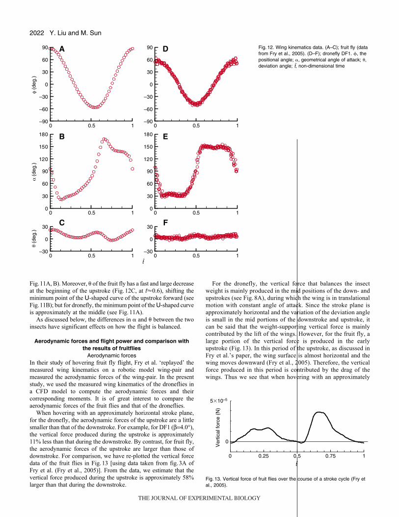
Fig.11A, B). Moreover, � of the fruit fly has a fast and large decrease

at the beginning of the upstroke (Fig.12C, at t�0.6), shifting the

minimum point of the U-shaped curve of the upstroke forward (see

Fig.11B); but for dronefly, the minimum point of the U-shaped curve

is approximately at the middle (see Fig.11A).

As discussed below, the differences in � and � between the two

insects have significant effects on how the flight is balanced.

Aerodynamic forces and flight power and comparison withthe results of fruitflies

Aerodynamic forcesIn their study of hovering fruit fly flight, Fry et al. ‘replayed’ the

measured wing kinematics on a robotic model wing-pair and

measured the aerodynamic forces of the wing-pair. In the present

study, we used the measured wing kinematics of the droneflies in

a CFD model to compute the aerodynamic forces and their

corresponding moments. It is of great interest to compare the

aerodynamic forces of the fruit flies and that of the droneflies.

When hovering with an approximately horizontal stroke plane,

for the dronefly, the aerodynamic forces of the upstroke are a little

smaller than that of the downstroke. For example, for DF1 (β=4.0°),

the vertical force produced during the upstroke is approximately

11% less than that during the downstroke. By contrast, for fruit fly,

the aerodynamic forces of the upstroke are larger than those of

downstroke. For comparison, we have re-plotted the vertical force

data of the fruit flies in Fig.13 [using data taken from fig.3A of

Fry et al. (Fry et al., 2005)]. From the data, we estimate that the

vertical force produced during the upstroke is approximately 58%

larger than that during the downstroke.

Y. Liu and M. Sun

For the dronefly, the vertical force that balances the insect

weight is mainly produced in the mid positions of the down- and

upstrokes (see Fig. 8A), during which the wing is in translational

motion with constant angle of attack. Since the stroke plane is

approximately horizontal and the variation of the deviation angle

is small in the mid portions of the downstroke and upstroke, it

can be said that the weight-supporting vertical force is mainly

contributed by the lift of the wings. However, for the fruit fly, a

large portion of the vertical force is produced in the early

upstroke (Fig. 13). In this period of the upstroke, as discussed in

Fry et al.’s paper, the wing surface is almost horizontal and the

wing moves downward (Fry et al., 2005). Therefore, the vertical

force produced in this period is contributed by the drag of the

wings. Thus we see that when hovering with an approximately

0 0.5 1–90

–60

–30

0

30

60

90

φ (d

eg.)

α (

deg.

)θ

(deg

.)

0 0.5 10

30

60

90

120

150

180

0 0.5 1–30

0

30

0 0.5 1–90

–60

–30

0

30

60

90

0 0.5 10

30

60

90

120

150

180

0 0.5 1–30

0

30

t

A

B

C

D

E

F

Fig. 12. Wing kinematics data. (A–C); fruit fly (datafrom Fry et al., 2005). (D–F); dronefly DF1. �, thepositional angle; �, geometrical angle of attack; �,deviation angle; t, non-dimensional time

Fig. 13. Vertical force of fruit flies over the course of a stroke cycle (Fry etal., 2005).

t

Ver

tical

forc

e (N

)

0 0.25 0.5 0.75 1

0

5�10–5



horizontal stroke plane, the dronefly mainly uses the lift principle

for the weight-supporting force, whilst the fruit fly uses both lift

and drag principles.

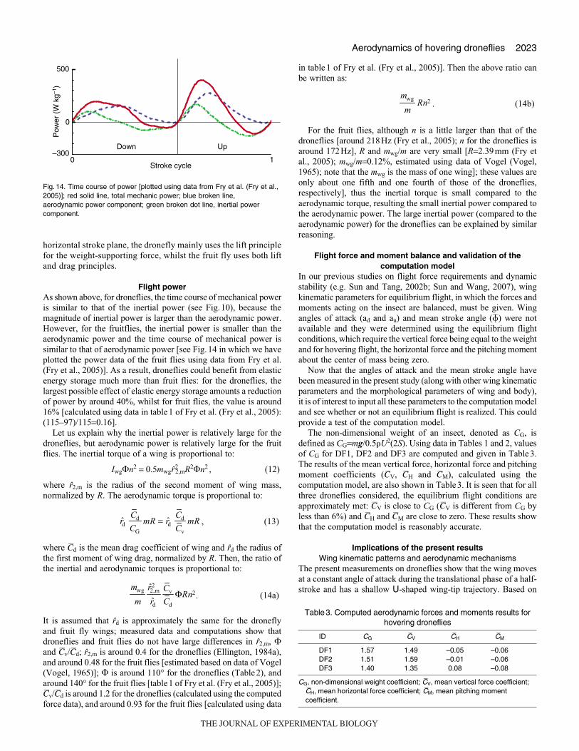
Flight powerAs shown above, for droneflies, the time course of mechanical power

is similar to that of the inertial power (see Fig.10), because the

magnitude of inertial power is larger than the aerodynamic power.

However, for the fruitflies, the inertial power is smaller than the

aerodynamic power and the time course of mechanical power is

similar to that of aerodynamic power [see Fig.14 in which we have

plotted the power data of the fruit flies using data from Fry et al.

(Fry et al., 2005)]. As a result, droneflies could benefit from elastic

energy storage much more than fruit flies: for the droneflies, the

largest possible effect of elastic energy storage amounts a reduction

of power by around 40%, whilst for fruit flies, the value is around

16% [calculated using data in table1 of Fry et al. (Fry et al., 2005):

(115–97)/115=0.16].

Let us explain why the inertial power is relatively large for the

droneflies, but aerodynamic power is relatively large for the fruit

flies. The inertial torque of a wing is proportional to:

Iwg�n2 = 0.5mwgr22,mR2�n2 , (12)

where r2,m is the radius of the second moment of wing mass,

normalized by R. The aerodynamic torque is proportional to:

where Cd is the mean drag coefficient of wing and rd the radius of

the first moment of wing drag, normalized by R. Then, the ratio of

the inertial and aerodynamic torques is proportional to:

It is assumed that rd is approximately the same for the dronefly

and fruit fly wings; measured data and computations show that

droneflies and fruit flies do not have large differences in r2,m, �and Cv/Cd; r2,m is around 0.4 for the droneflies (Ellington, 1984a),

and around 0.48 for the fruit flies [estimated based on data of Vogel

(Vogel, 1965)]; � is around 110° for the droneflies (Table2), and

around 140° for the fruit flies [table1 of Fry et al. (Fry et al., 2005)];

Cv/Cd is around 1.2 for the droneflies (calculated using the computed

force data), and around 0.93 for the fruit flies [calculated using data

. (14a)

mwg

m

r̂2,m2

r̂d

Cv

Cd

ΦRn2

, (13) r̂d

Cd

CG

mR = r̂dCd

Cv

mR

in table1 of Fry et al. (Fry et al., 2005)]. Then the above ratio can

be written as:

For the fruit flies, although n is a little larger than that of the

droneflies [around 218Hz (Fry et al., 2005); n for the droneflies is

around 172Hz], R and mwg/m are very small [R=2.39mm (Fry et

al., 2005); mwg/m=0.12%, estimated using data of Vogel (Vogel,

1965); note that the mwg is the mass of one wing]; these values are

only about one fifth and one fourth of those of the droneflies,

respectively], thus the inertial torque is small compared to the

aerodynamic torque, resulting the small inertial power compared to

the aerodynamic power. The large inertial power (compared to the

aerodynamic power) for the droneflies can be explained by similar

reasoning.

Flight force and moment balance and validation of thecomputation model

In our previous studies on flight force requirements and dynamic

stability (e.g. Sun and Tang, 2002b; Sun and Wang, 2007), wing

kinematic parameters for equilibrium flight, in which the forces and

moments acting on the insect are balanced, must be given. Wing

angles of attack (ad and au) and mean stroke angle (�) were not

available and they were determined using the equilibrium flight

conditions, which require the vertical force being equal to the weight

and for hovering flight, the horizontal force and the pitching moment

about the center of mass being zero.

Now that the angles of attack and the mean stroke angle have

been measured in the present study (along with other wing kinematic

parameters and the morphological parameters of wing and body),

it is of interest to input all these parameters to the computation model

and see whether or not an equilibrium flight is realized. This could

provide a test of the computation model.

The non-dimensional weight of an insect, denoted as CG, is

defined as CG=mg/0.5�U2(2S). Using data in Tables 1 and 2, values

of CG for DF1, DF2 and DF3 are computed and given in Table3.

The results of the mean vertical force, horizontal force and pitching

moment coefficients (CV, CH and CM), calculated using the

computation model, are also shown in Table3. It is seen that for all

three droneflies considered, the equilibrium flight conditions are

approximately met: CV is close to CG (CV is different from CG by

less than 6%) and CH and CM are close to zero. These results show

that the computation model is reasonably accurate.

Implications of the present resultsWing kinematic patterns and aerodynamic mechanisms

The present measurements on droneflies show that the wing moves

at a constant angle of attack during the translational phase of a half-

stroke and has a shallow U-shaped wing-tip trajectory. Based on

. (14b)

mwg

mRn2

Pow

er (

W k

g–1)

0

500

0 1

Down Up–300

Stroke cycle

Fig. 14. Time course of power [plotted using data from Fry et al. (Fry et al.,2005)]; red solid line, total mechanic power; blue broken line,aerodynamic power component; green broken dot line, inertial powercomponent.

Table3. Computed aerodynamic forces and moments results forhovering droneflies

ID CG CV CH CM

DF1 1.57 1.49 –0.05 –0.06DF2 1.51 1.59 –0.01 –0.06DF3 1.40 1.35 0.08 –0.08

CG, non-dimensional weight coefficient; CV, mean vertical force coefficient;CH, mean horizontal force coefficient; CM, mean pitching momentcoefficient.


2024

the wing kinematic pattern, analysis using the CFD model shows

that the droneflies primarily use lift to produce weight-supporting

force during the translational phase (via the delayed stall

mechanism).

Fry et al.’s measurements on fruit flies (Fry et al., 2005) showed

a very different wing kinematic pattern: the wing had a large

downward plunge at the start of a half-stroke, resulting in a deep

U-shaped wing-tip trajectory. Based on this wing kinematics, their

experimental study using a robotic wing showed that the fruit flies

rely heavily on drag mechanism during stroke reversal in producing

vertical force.

These results demonstrate that insects having different wing

kinematic patterns may employ different aerodynamic mechanisms

for flight, and that in order to reveal the aerodynamic mechanisms

an insect uses, detailed wing kinematics measurements should be

conducted first. It is suggested that the studies on hovering of fruit

flies (Fry et al., 2005) and droneflies (present study) are extended

to other flight modes, such as forward flight and maneuver, and

later on, other representative insects should be studied.

CFD method, combined with detailed kinematics measurements: atool of great promise

An advantage of the CFD method in the study of insect flight

aerodynamics and dynamics is that when the computational code

is validated for an insect in a certain flight mode (for example,

hovering), it can be readily used for other flight modes and for other

insects. When changing from hovering to forward flight or other

flight modes, only the input boundary conditions, determined by

the wing motion, need to be changed, and this can be easily

accomplished. When the code is used for other insects, the wing

shape, hence the computational grid, and the Reynolds number in

the Navier–Stokes equations need to be changed (Wu and Sun,

2004); both can be accomplished without much difficulty.

A second advantage is that the CFD method can provide any

physical quantities that are needed for flow analysis. For example,

aerodynamic force distribution on the wing is available, thus total

aerodynamic force, moment about the center of mass of body (for

flight balance study), and moment about wing root (for power

calculation) can be readily obtained. Another example is that

streamline patterns and vortices in the flow can be easily

visualized.

The CFD model in the present study has been successfully

validated for hovering droneflies. As discussed above, it can be

readily used for study of other flight modes of droneflies and flight

of other insects, provided that detailed wing kinematic patterns are

measured. Combined with the method of 3D high-speed

videography, the CFD method could be a tool of great promise in

the future study of insect flight aerodynamics and dynamics.

LIST OF ABBREVIATIONS AND SYMBOLSc mean chord length

CD wing drag coefficient

CG weight coefficient

CH horizontal force coefficient

CH mean horizontal force coefficient

CL wing lift coefficient

CM pitching moment coefficient

CM mean pitching moment coefficient

CP non-dimensional power

CV vertical force coefficient

CV mean vertical force coefficient

Cw non-dimensional work per cycle

Cw+ non-dimensional positive work per cycle

Cw– non-dimensional negative work per cycle

Y. Liu and M. Sun

CFD computational fluid dynamics

D drag of a wing

g the gravitational acceleration

h1 distance from wing-root axis to long-axis of body

H horizontal force

Iwg moment of inertia of the wing about wing root

Iy moment of inertia of the body about center of mass

J advance ratio

lb body length

lr distance between two wing roots

l1 distance from wing-root axis to body center of mass

L lift of a wing

LED light emitting diode

m mass of an insect

mwg mass of one wing

Ma aerodynamic moment of wing around wing root

Mi inertial moment of wing around wing root

My pitching moment about center of mass

n stroke frequency

Pa aerodynamic power

Pi inertial power

P* body-mass-specific power

r2 radius of the second moment of wing area

r2,m radius of the second moment of wing mass

rd radius of the first moment of wing drag

R wing length

S area of one wing

t time

tc period of wing beat

t non-dimensional time (t=0 and 1 at the start and end of a

cycle, respectively)

U reference velocity (mean flapping velocity at r2)

V vertical force of a wing

� angle of attack

�d constant value of � at the mid-position of the downstroke

�u constant value of � at the mid-position of the upstroke

stroke plane angle

�tp non-dimensional time duration for pronation

�tp,t non-dimensional advance time for pronation

�ts non-dimensional time duration for supination

�ts,t non-dimensional advance time for spination

1 phase angle of the first harmonic of Fourier series of deviation

angle

2 phase angle of the second harmonic of Fourier series of

deviation angle

� deviation angle

�0 constant value of Fourier series of deviation angle

�1 amplitude of the first harmonic of Fourier series of deviation

angle

�2 amplitude of the second harmonic term of deviation angle

� density of fluid

� kinematic viscosity of fluid

� positional angle

� mean positional angle

� stroke amplitude

� body angle

�0 free body angle

wing rotation velocity vector

This research was supported by the National Natural Science Foundation ofChina (10732030).

REFERENCESDickinson, M. H., Lehmann, F. O. and Sane, S. P. (1999). Wing rotation and the

aerodynamic basis of insect flight. Nature 284,1954-1960.Dudley, R. and Ellington, C. P. (1990). Mechanics of forward flight in bumblebees. I.

Kinematics and morphology. J. Exp. Biol. 148, 19-52.Ellington, C. P. (1984a). The aerodynamics of hovering insect flight. II. Morphological

parameters. Philos. Trans. R. Soc. Lond. B Biol. Sci. 305, 1-15.Ellington, C. P. (1984b). The aerodynamics of hovering insect flight. III. Kinematics.

Philos. Trans. R. Soc. Lond. B Biol. Sci. 305, 17-40.Fry, S. N., Sayaman, R. and Dickinson, M. H. (2005). The aerodynamics of hovering

flight in Drosophila. J. Exp. Biol. 208, 2303-2318.



Lehmann, F. O., Sane, S. P. and Dickinson, M. H. (2005). The aerodynamiceffects of wing–wing interaction in flapping insect wings. J. Exp. Biol. 208, 3075-3092.

Sun, M. and Tang, J. (2002a). Unsteady aerodynamic force generation by a modelfruit fly wing in flapping motion. J. Exp. Biol. 205, 55-70.

Sun, M. and Tang, J. (2002b). Lift and power requirements of hovering flight inDrosophila virilis. J. Exp. Biol. 205, 2413-2427.

Sun, M. and Wang, J. K. (2007). Flight stabilization control of a hovering modelinsect. J. Exp. Biol. 210, 2714-2722.

Sun, M. and Yu, X. (2006). Aerodynamic force generation in hovering flight in a tinyinsect. AIAA J. 44, 1532-1540.

Usherwood, J. R. and Ellington, C. P. (2002a). The aerodynamics of revolving wings.I. Model hawkmoth wings. J. Exp. Biol. 205, 1547-1564.

Usherwood, J. R. and Ellington, C. P. (2002b). The aerodynamics of revolving wings.II. Propeller force coefficients from mayfly to quail. J. Exp. Biol. 205, 1565-1574.

Vogel, S. (1965). Flight in Drosophila I. Flight performance of tethered flies. J. Exp.Biol. 44, 567-578.

Willmott, A. P. and Ellington, C. P. (1997). The mechanics of flight in the hawkmothManduca sexta. I. Kinematics of hovering and forward flight. J. Exp. Biol. 384, 2705-2722.

Wu, J. H. and Sun, M. (2004). Unsteady aerodynamic forces of a flapping wing. J.Exp. Biol. 207, 1137-1150.


Documents

Wing kinematics measurement and aerodynamics of hovering droneflies.pdf