Wishful Thinking∗

Andrew Caplin†and John Leahy‡

October 2018Preliminary and Incomplete

Abstract

We model agents who get utility from their beliefs and therefore interpret informa-

tion optimistically. They exhibit several biases observed in psychoglical studies such as

optimism, confirmation bias, polarization, and the endowment effect. In some formu-

latins, they exhibit these biases even though they are subjectively Bayesian. We show

that wishful thing can lead to reduced saving, make possible information-based trade,

and generate asset bubbles.

“For a man always believes more readily that which he prefers”Francis Bacon (1620)

1 Introduction

Expectation formation is central to many economic questions. Workers must form expec-

tations regarding retirement. Investors must form expectations of risk and return. Price

setters must form expectations of competitor’s prices. While expectations are central, we

do not fully understand how expectations are formed. The typical approach is to assume

that expectations are model consistent. Agents understand the world in which they live and

∗We thank Anmol Bhandari, Wouter den Haan, Behzad Diba, Jordi Gali, Nicola Pavoni, Kaitlin Raimi,Matthew Shapiro, Allen Sinai, Linda Tesar, and Jaume Ventura for helpful discussions.†Center for Experimental Social Science and Department of Economics, New York University. Email:

andrew.caplin@nyu.edu‡Department of Economics and Gerald R Ford School of Public Policy, University of Michigan and NBER.

Email: jvleahy@umich.edu

1

form expectations rationally. There is a lot of psychological evidence, however, that agents

are poor information aggregators. They are often over-confident. They tend to interpret

information in accordance with their priors. Beliefs seem to be sensitive to rewards. It is

therefore of interest to develop models of belief formation that go beyond the assumption of

rational expectations.

In this paper, we proceed in the spirit of Becker and model beliefs as a choice. Agents

choose beliefs that raise their subjective utility subject to a cost. This desire to “see the world

through rose colored glasses”naturally leads to several apparent deviations from rationality

such as optimism, procrastination, confirmation bias, and polarization. We illustrate the

economic implications in a series of simple examples and models. We show how wishful

thinking may reduce saving and create bubbles. We show how wishful thinkers may engage

in information based trade.

Any model of belief choice must specify the costs and the benefits of distorting beliefs. In

the standard economic model, there is no benefit to believing anything other than the truth.

Agents get utility from outcomes, and probabilities serve only to weight these outcomes.

Getting the probabilities wrong muddles one’s view of the payoffs to an action and leads to

mistakes. In the standard model, there are strong incentives to have accurate beliefs, since

accurate beliefs lead to accurate decisions.

To model the benefits of belief choice we follow Jevons (1905), Loewenstein (1987) and

Caplin and Leahy (2001) and assume that some portion of utility depends on the anticipation

of future outcomes. Anxiety, fear, hopefulness and suspense are all ways in which beliefs

about the future affect wellbeing today. The American Psychiatric Association defines anx-

iety as “apprehension, tension, or uneasiness that stems from the anticipation of danger.”

The dependence of current wellbeing on beliefs about the future creates an incentive to be-

lieve that “good”outcomes are more likely than “bad”outcomes. Wishful thinking involves

choosing to believe that the truth is what one would like the truth to be.

Without constraints a theory of belief choice would lack content. One could believe

anything one liked. Our model of the constraints rests on the idea that there are often lots of

possible beliefs that are consistent with experience. We limit our agents to “plausible”beliefs,

by which we mean beliefs that are not obviously contradicted by the available evidence. We

follow Hansen and Sargent (2008) and impose a cost to beliefs that are too far away from

the truth, where we associate the truth with the beliefs that an objective observer would

hold. This cost is related to the Kullback-Leibler divergence from the agent’s subjective

beliefs to the objective probability distribution. The Kullback-Leibler divergence measures

2

the likelihood that the subjective beliefs would be rejected in favor of the objective ones.

The more unlikely the truth, the more costly the beliefs.

The outcome is a model of belief choice. Optimal beliefs tend to twist the probabilities

in the direction of events with high utility. The upper bound on probabilities limits wishful

thinking about very likely events. Events can only be so likely. While unlikely events with

high payoffs receive more weight, wishful thinking is not magical thinking. Low probability

events remain low probability, and zero probability events remain zero probability. Wishful

thinking is strongest when payoff differences are large and outcomes are uncertain. Such

situations might plausibly include choices that are made infrequently so that the agent lacks

experience with them such as saving for retirement. They might also include situations in

which the options are diffi cult to value such as the valuation of real estate where every house

is in some sense a unique asset and few houses trade at any given time. They might include

any situation in which there are multiple theories on the table and very little evidence to

distinguish between them as is often the case with asset bubbles.1

We present two formulations of the cost function which differ as to how beliefs are chosen.

In the first formulation, we allow agents to directly choose their posterior beliefs. The first

formulation is simpler, and allows us to directly incorporate many of the tools developed by

Hansen and Sargent (2008) to study robust control. The first formulation leads to optimism

and over-confidence as agents overstate the probability of having chosen the correct answer.

Wishful thinkers, in this formulation, tend to value uncertainty as it opens up the possibility

of wishful thinking. They tend to prefer the late resolution of uncertainty. This can lead

them to delay actions when the future is uncertain, which can explain procrastination. It

also can lead them to take actions that are themselves uncertain, which can help explain

bubbles.

In the second formulation, we allow agents to choose how they interpret signals which

then enter into their posterior beliefs. This formulation is mathematically more complicated,

but gives rise to a richer set of apparent deviations from rationality. In addition to optimism

and procrastination, agents appear to twist information in the direction of their priors, a

phenomenon known as confirmation bias. After observing the same information, two agents

with divergent priors may also come to hold these divergent beliefs more strongly, a phe-

nomenon known as polarization. This second formulation has the additional distinction that

these apparent deviations from rationality all occur in a model in which agents are subjec-

tive Bayesians. In this formulation, they accurately combine subjective signals with priors to

1Reinhart and Rogoff title their study of credit booms "This Time is Different", emphasizing that thereare mulitple interpretations of the evidence and a tendency to gravitate towards the optimistic ones.

3

form subjective posteriors, so that their subjective reality is rational. Their problem is that

is that their subjective interpretation of the signals differs from the objective counterpart.

While subjectively Bayesian, they will appear non-Bayesian to an objective observer. We

label the first formulation the cumulative model since the cost is on the sum of all accumu-

lated information, and we label the second formulation the flow model since the cost is on

the flow of new information.

We present three economic implications of wishful thinking. First, we extend the cumu-

lative model to a dynamic setting and present a simple model of consumption and saving

in the presence of idiosyncratic income risk in the style of Huggett (1993). The economy is

populated by both wishful thinkers and objective agents. We show that the wishful thinkers

tend to place relatively high weight on high utility states which also tend to be the low

marginal utility states. This leads them to consume more and save less, and therefore end

up with less accumulated wealth. Second, we show that our setting is outside of the class

of models considered by Milgrom and Stokey (1982). We present an example in which a

wishful thinker and an objective agent actively trade based on private information. In the

example, agents do not hold their beliefs dogmatically. They learn from the other agent’s

desire to trade. Nevertheless they agree to disagree. The wishful thinker knows the beliefs

of the objective agent but chooses to believe differently. Third, we present a model of asset

bubbles. We consider the introduction of a new and uncertain technology and show that the

wishful thinkers will bid its price above its fundamental value, where fundamental value is

determined by the valuation of the objective agents. We map our description of a bubble to

the narrative in Kindelberger (1978).

Our premise is that people shade their beliefs in ways that make their choices look better.

There is evidence that supports this assertion. In a classic study of cognitive dissonance,

Knox and Inkster (1968) interviewed bettors at a race track and found that bettors placed

higher odds on their preferred horse when interviewed after placing their bets than bettors

did when interviewed while in line waiting to place their bets. Knox and Inkster attribute this

phenomenon to a desire to reduce post-decision dissonance, that is a desire to match one’s

world view with ones decisions. Mijovic-Prelec and Prelec (2010) perform a similar analysis

in a controlled experimental setting. They had subjects make incentivized predictions before

and after being given stakes in the outcomes, and found that there was a tendency for subjects

to reverse their predictions when the state that they had predicted to be less likely turned

out to be the high payoff state. Bastardi, Uhlmann, and Ross (2011) conduct a standard

test of confirmation bias, but instead of focusing on the relationship between a subject’s

prior beliefs and their interpretation of evidence, they instead focus on the subject’s prior

4

decisions. They consider a population of parents who profess to believe that home care is

superior to day-care for their children. Some, however, have chosen home care, whereas

others, because they have jobs, have been forced to choose day-care. They present this

population with two fictional studies, one of which claims home care is superior and one

which claims day-care is superior. Confirmation bias would predict that all parents would

rate the former study as superior since all parents share the same prior beliefs. Instead, the

parents who had placed their children in day-care rated the study supporting day-care as

superior, whereas the parents who cared for their children at home did the opposite. Some

of the parents who had placed their children in day-care changed their beliefs and professed

day-care was no worse than home care. The authors conclude that the parents choose to

believe what they want to believe.

Section 2 discusses related literature. Section 3 presents the cumulative model. Section 4

presents the flow model. Section 5 discusses the economic applications. Section 6 discusses a

number of issues, including alternative modeling choices and the relationship to the literature

on robust control. Section 7 concludes.

2 Related Literature

We contribute to three literatures. The first is the literature on belief choice which is surveyed

by Benabou and Tirole (2016). They divide the literature into two classes depending on the

motivation for distorting one’s beliefs. In one class, beliefs enter directly into utility. In the

other beliefs are instrumental in motivating desirable actions or achieving desirable goals.

For example, beliefs may aid in overcoming self-control problems, signaling one’s type, or

fostering commitment. Our paper fits into the first class. Akerlof and Dickens (1982) is

a prominent early contribution to this literature. They present the example of an agent

considering a job in a hazardous industry. Upon accepting the job the agent may choose to

understate the probability of an accident in their industry. This is desirable since it reduces

fear, and fear reduces utility in their model. The cost of distorting beliefs is that mistaken

beliefs may lead to suboptimal decision s in subsequent periods. For example, the agent may

choose to forgo safety equipment if they believe that the risk of an accident is low. Akerlof

and Dickens constrain the subjective probability of an accident to be less than the objective

probability. The linearity of the model leads to bang-bang solutions depending whether the

cost or the benefit is greater. They assume that the agent evaluates these options with the

true probabilities when considering belief choice. Brunnermeier and Parker (2005) is another

closely related paper. They assume that an agent can choose their prior at the beginning of

5

their life, and then given this prior behaves as a Bayesian in all subsequent periods. They

model belief choice as balancing the gain to anticipating a more positive future and against

the cost of suboptimal decisions. Like Akerlof and Dickens the agent evaluates belief choice

using the true probability distribution, and then proceeds with the chosen beliefs. We discuss

the relationship between our model and Brunnermeier and Parker’s in detail in Section 6

below.

A second literature is the literature on anticipatory utility. Jevons (1905), Loewenstein

(1987) and Caplin and Leahy (2001, 2004) all suppose that current happiness depends in

some way on beliefs regarding future outcomes. Jevons believed that agents acted only to

maximize current happiness. Intertemporal optimization, in this view, maximized the sum

of the happiness from actions today and the current happiness arising from the anticipation

of future actions. Loewenstein builds a model to explain why an agent might wish to bring

forward an unpleasant experience to shorten the period of dread, or to postpone a pleasant

experience in order to savor the anticipation. Caplin and Leahy model emotional responses

to future risks such as anxiety, suspense, hope, and fear. Brunnermeier and Parker build on

the utility function in Caplin and Leahy.

Our paper also contributes to the recent explosion of work that deviates from rational

expectations. A partial and incomplete selection includes the following. Hansen and Sar-

gent (2008) consider robust expectations that incorporate a fear of model mis-specification.

Fuster, Laibson, and Mendel (2010) propose what they call “natural expectations”which

involve a weighted average of rational expectations and the prediction of a simple linear

forecasting model. Gabaix (2014) considers a “sparsity-based”model in which agents place

greater weight on variables that are of greater importance. Burnside, Eichenbaum and Re-

belo (2016) develop a model in which the distribution of expectations in the economy are

influenced by social dynamics. Bordalo, Gennaioli, and Schleifer (2018) consider what they

call “diagnostic expectations”. These are based on what psychologists call the representative

heuristic and involve an overweighting of outcomes that are becoming more likely. Another

related paper is Mullainathan and Schlifer (2005) who model how a preference for biased

information affects the supply of information that produced by the news media.

3 A Simple Model of Belief Choice

We begin with the cumulative information model in which the agent chooses their posterior

beliefs and discuss the flow model in the next section. The essential elements of both theories

6

are: (1) a decision whose outcome is unknown; (2) objective probabilities of the outcome;

(3) utility from beliefs regarding the outcome; and (4) a cost to choosing beliefs that differ

from the objective probabilities. We discuss these elements in turn.

There are two periods. In the first period, an agent chooses an action a from a finite

set of potential choices A. In the second period, nature selects a state ω from a finite set

of potential states of the world Ω. There is an objective probability distribution over the

second-period states γ ∈int∆(Ω), which we associate with the beliefs of an objective observer.

We follow Jevons (1905) and assume that the agent maximizes their current subjective

expected utility. Current subjective expected utility incorporates both utility from current

experience and utility from the anticipation of future outcomes. For simplicity we abstract

from the former and focus solely on the anticipation of the future. We break down the utility

from the anticipation into two components. The first is the payoff that the agent anticipates

receiving in state ω should they choose action a, which we denote u(a, ω). The second is the

agents’subjective probability that state ω will occur, which we denote γ(ω). We assume the

agent understands their preferences so that they have an accurate assessment of u(a, ω).2 γ,

however, will generally differ from γ and may depend on the action choice a. The agent’s

subjective expected utility from the action a is:3 ,4∑ω∈Ω

γ(ω)u(a, ω) (1)

Maximizing (1) generates an incentive to choose beliefs. We discipline this choice with a

cost. Rather than model the specific technology by which beliefs are distorted, for example

by selective memory, selective attention, or self-signalling, we hypothesize that the costs of

belief distortion are increasing in the size of the distortion.5 We follow Hansen and Sargent

(2008) and relate the cost of choosing γ(ω) to the Kullback-Leibler divergence from γ(ω) to

2Nothing is lost in assuming that the agent cannot manipulate their beliefs regarding u(a, ω). We caninterpret ω broadly as including the quality of the match between the agent and the action a. An increasein the probability of a good match is equivalent to an increase in u(a, ω).

3The advantage of Jevon’s formulation is that the objective probabilities do not enter this calculation.The agent does not directly care about their future self and therefore does not consider the potential costsof mistaken beliefs as they do in the models of Akerlof and Dickens (1982) and Brunnermeier and Parker(2005). An interesting way forward is incorporate a concern for future mistakes into the model.

4The agent receives utility from the action a both through prior anticipation and eventual experience.In Jevons’view, only the former influences choice. In dynamic models with multiple periods choice is timeconsistent if anticipatory utility mirrors experienced utility and the agent discounts the anticipation of futureutility exponentially. Optimal policy invloves additional complications. See Caplin and Leahy (2006).

5See Benebou and Tirole (2016) for a discussion of theories of selective memory, selective attention andself-signalling.

7

γ(ω). The cost is1

θ

∑ω∈Ω

γ(ω) lnγ(ω)

γ(ω)(2)

This cost (2) is the expected likelihood ratio under the subjective measure γ. It measures

the ability of the agent to discriminate between γ and γ given that the agent believes that

the signal is γ. The idea is that it is easier to choose a subjective belief that is not wildly

contradicted by experience.

This cost function provides the link between the agent’s subjective reality γ and the

outside world γ. We will think of γ as reflecting the objective view of an unbiased expert.

Agents understand what the expert is saying, but are aware that experts are not all knowing

and are frequently wrong. Even in the best of cases, estimates of models come with standard

errors. The cost function states that beliefs become harder and harder to justify, the further

they are from expert opinion.

An alternative interpretation of the model is there exists a collection of experts with

differing views. Such would be the case with many fundamental macroeconomic questions

such as size of the fiscal multiplier, the slope of the Phillips curve, or the level of the natural

rate of unemployment. In these cases, there is no consensus on the true structural model and

experts come to vastly different conclusions. In this interpretation, γ represents mainstream

opinion. The agent chooses an expert and sees an increasing cost to choosing an expert that

deviates too far from the consensus. In this interpretation, γ need not reflect the “truth”or

“objective opinion. Instead γ might reflect the prevailing orthodoxy and the cost function

might reflect the cost of deviating from this orthodoxy.6

The parameter θ captures the ease with which the agent can manipulate their beliefs.

The larger is θ the greater the amount of evidence the agent would need before they reject

their chosen beliefs in favor of the objective ones. When θ is equal to infinity, any beliefs are

possible. When θ is equal to zero, any deviation from γ comes at an infinite cost.

Summarizing the above, the agent’s maximization problem becomes

V (γ) = maxγ∈int∆(Ω),a∈A

∑ω∈Ω

γ(ω)u(a, ω)− 1

θ

∑ω∈Ω

γ(ω) lnγ(ω)

γ(ω). (3)

The first term is the subjective expected utility of choice a. The second term is the cost of

the believing γ. Implicit in the maximization problem (3) is the assumption that the agent

6If we take this view then an interesting way forward is to endogenize the supply of experts along thelines of Mullainathan and Schlifer (2005) .

8

understands that their beliefs γ will depend on the choice a. We consider the implications

of assuming that the agent is naive in Section 6.

The maximization problem (3) is very similar to the robust control problem in Hansen

and Sargent (2008). There are two differences. First, Hansen and Sargent maximize over a

and conditional on a minimize over γ. Second, because Hansen and Sargent minimize over

γ, they add rather than subtract the cost (2). This is equivalent to replacing θ with −θ. Itis therefore not surprising that many of our conclusions will be exactly the opposite of those

of Hansen and Sargent.

3.1 Implications for belief choice

Given that the agent understands the interaction between belief choice and action choice,

it does not matter whether the agent chooses beliefs and then actions or actions and then

beliefs. We will therefore fix the action and focus, for the time being, on belief choice. Given

that the action a is fixed, we write u(ω) for u(a, ω). The first order condition for γ(ω) implies

γ(ω) =γ(ω) exp [θu(ω)]∑

ω′∈Ω γ(ω′) exp [θu(ω′)](4)

According to (4), the agent distorts their beliefs. They tend to increase the probability of

states with high utility and they reduce the probability of states with low utility.

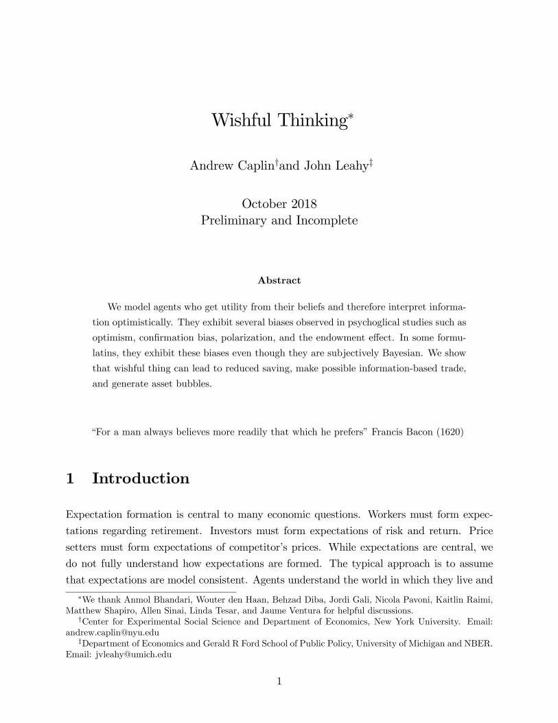
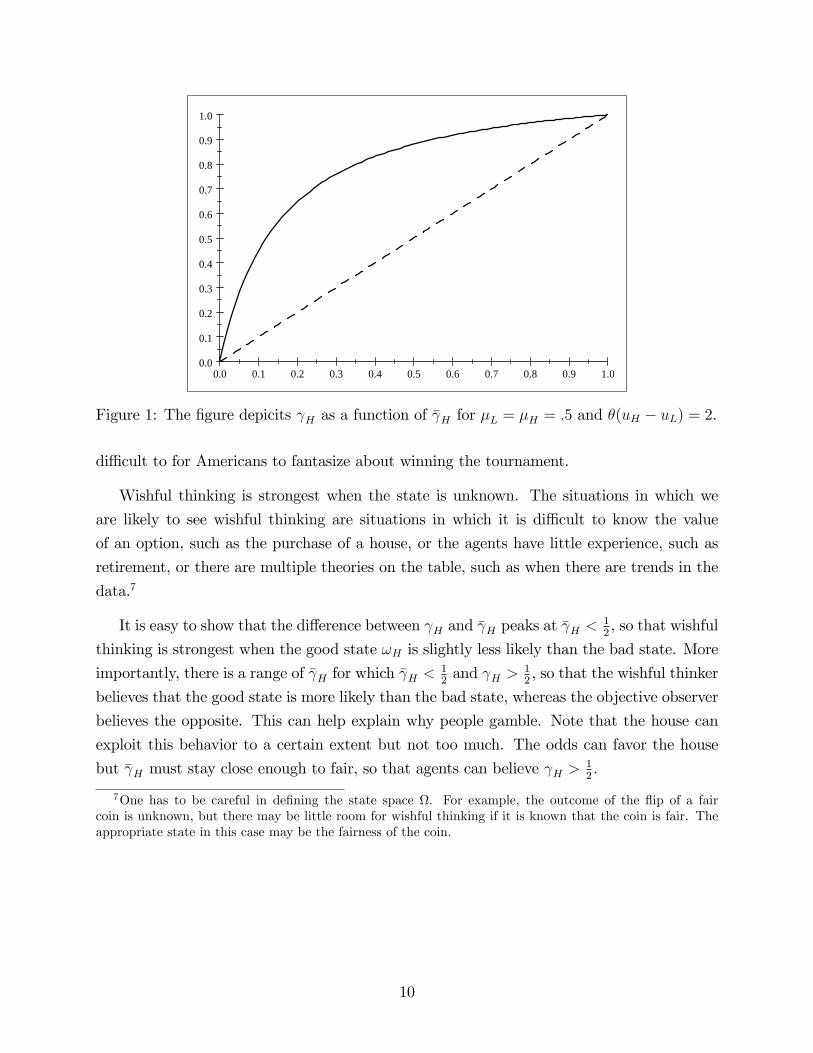
Figure 1 graphs γ(ω) as a function of γ(ω) for an example with two states: a high utility

state ωH in which utility is uH and a low utility state ωL with utility uL The objective

probability of the high utility state is on the horizontal axis. The solid line represents the

chosen probability as measured on the vertical axis. The dashed line is the 45 degree line.

The gap between the two lines represents the extent of wishful thinking,

γH − γH =γH γL (exp [θuH ]− exp [θuL])

γH exp [θuH ] + γL exp [θuL]

Since the ωH is the good state, exp [θuH ]−exp [θuL] > 0 and this gap is everywhere positive.

The constraint that probabilities are less than one, limits the amount of wishful thinking

when the good state is very likely. It is hard to be over-optimistic about a near certain event.

For example, Germans may be optimistic about their team’s chances to win the FIFA world

cup, but this does not necessarily reflect wishful thinking. Similarly, it is hard to be too

optimistic about very uncertain events. Wishful thinking is not magical thinking. If γH is

zero, then γH is zero too. Once the US team has been eliminated from the world cup, it is

9

0.0 0.1 0.2 0.3 0.4 0.5 0.6 0.7 0.8 0.9 1.00.0

0.1

0.2

0.3

0.4

0.5

0.6

0.7

0.8

0.9

1.0

Figure 1: The figure depicits γH as a function of γH for µL = µH = .5 and θ(uH − uL) = 2.

diffi cult to for Americans to fantasize about winning the tournament.

Wishful thinking is strongest when the state is unknown. The situations in which we

are likely to see wishful thinking are situations in which it is diffi cult to know the value

of an option, such as the purchase of a house, or the agents have little experience, such as

retirement, or there are multiple theories on the table, such as when there are trends in the

data.7

It is easy to show that the difference between γH and γH peaks at γH < 12, so that wishful

thinking is strongest when the good state ωH is slightly less likely than the bad state. More

importantly, there is a range of γH for which γH < 12and γH > 1

2, so that the wishful thinker

believes that the good state is more likely than the bad state, whereas the objective observer

believes the opposite. This can help explain why people gamble. Note that the house can

exploit this behavior to a certain extent but not too much. The odds can favor the house

but γH must stay close enough to fair, so that agents can believe γH > 12.

7One has to be careful in defining the state space Ω. For example, the outcome of the flip of a faircoin is unknown, but there may be little room for wishful thinking if it is known that the coin is fair. Theappropriate state in this case may be the fairness of the coin.

10

3.2 Action Choice

We can calculate the value of the action a under the optimal beliefs. Substituting (4) into

V (γ) for a given action choice a yields

V (γ) = maxa

1

θ

(ln∑ω

γ(ω)eθu(a,ω)

)(5)

This has the form of Epstein-Zin (1989) preferences, f−1(Ef(u(ω)) where f(x) = exp(x).

Given that exp(x) is convex, the agent has a preference for late resolution to uncertainty.

This is not surprising as it is uncertainty that allows the agent to engage in wishful thinking.8

3.3 Overconfidence

Debondt and Thaler (1995) write, “Perhaps the most robust finding in the psychology of

judgement is that people are overconfident.”Experimental tests of overconfidence take several

forms. In one type of experiment, an agent is asked to choose the correct answer from a

set of potential answers and then asked their subjective probability of getting the correct

answer. In this case, overconfidence takes the form of optimism and arises when the subject’s

subjective probability of being correct exceeds the observed frequency with which they in

fact answer correctly. Another set of experiments asks for a numerical answer to a question

and for a subjective confidence interval. In this case, overconfidence takes the form of excess

precision and arises when the correct answer fails to lie in the subjective confidence interval

as often as believed.

The spirit of these tests can be captured in a tracking problem in which the agent must

guess the state after receiving a signal. Suppose that there are N states labeled ω1 through

ωN equally spaced around a circle, so that the distance between ω1 and ω2 is equal to

the distance between ω1 and ωN . Nature picks the true state ω ∈ Ω, and the agent picks

a ∈ Ω. Let δ(a, ω) denote the minimum distance (about the circle) between the true state

and the choice and suppose that u depends only on δ: u(a, ω) = u(δ(a, ω)). This payoff

function captures both types of experiment. In the first case, there is a correct answer and

a collection of incorrect answers: u(δ) = 1 if δ = 0 and u(δ) = 0 otherwise. In the second

case, the loss is increasing in the δ. Suppose that the objective expert has a uniform prior

8While we have modeled an agent who distorts their beliefs, choice in this model turns out to be obser-vationally equivalent to the choice of an agent with distorted utility. The only way to test for the differencebetween these two settings would be to combine data on choice and beliefs.

11

over the states and receives a signal s ∈ Ω that has an objective density that is symmetric

about the true state and declining in the distance from the true state. The symmetry

of the prior and the signal imply that the experts beliefs are symmetric about the signal:

γ(ω|ω = s+ x) = γ(ω|ω = s− x) for all x.

Given the symmetry of the problem, the optimal choice is obvious: the agent simply

reports the signal: a = s. The question that we focus on is what the agent chooses to

believe. The first-order condition (4) becomes

γ(ω) =γ(ω) exp [θu(δ(s, ω))]∑ω′ γ(ω′) exp [θu(δ(s, ω))]

. (6)

Without loss of generality label the signal state ω0. Label the states to the right of ω0 (as

we move about the circle): ω1, ω2,..., and label the states to the left ω−1, ω−2,... If there

are an odd number of states keep the number of states with positive and negative indices

equal. If there are an even number of states, label the state furthest from ω0, ωN/2. With

this labeling, the absolute value of the index is equal to δ(s, ω). Now consider the ratio

γ(ωm)

γ(ωn)=γ(ωm) exp [θu(|m|)]γ(ωn) exp [θu(|n|))]

First, γ(ωn) = γ(ω−n) implies γ(ωn) = γ(ω−n), so that γ inherits the symmetry of γ.

Second, since u is maximized at δ = 0, γ(ω0)γ(ωn)

> γ(ω0)γ(ωn)

for all ωn 6= ω0. It follows immediately

that γ(ω0) > γ(ω0), so that the agent is over-optimistic that they have selected the correct

state. Finally, if we consider any subset of states relatively close to ω0, Ω = ωn s.t. |n| < N,γ(ωn)γ(ωm)

> γ(ωn)γ(ωm)

for any ωn ∈ Ω and ωm 6∈ Ω. Hence the agent will be overconfident that the

true state is in Ω. It follows that the agent will be over-confident in the sense that their

subjective confidence intervals will be too tight.

3.4 Procrastination and Self-Control

An example illustrates how the model generates procrastination. Consider the decision

problem in Figure 2. There are three periods represented by the nodes A, B, and C. In thefirst period (node A), the agent chooses whether to take an action or delay. The cost of theaction is 1. If the agent delays, then the agent is either free or busy in period 2 (node B).If the agent is free, they take the action in period 2 at a cost of 1/2. If they are busy, they

delay the action until period 3 (node C) and take the action at a cost of 2. The agent wishesto minimize costs.

12

[Insert Figure 2]

If we assume that it is equally likely that the agent is free or busy in period 2, then

an objective agent would calculate the expected cost of delay in period 1 to be 5/4. The

objective agent would then choose to act in period 1. What would a wishful thinker do?

Conditional on delay in period 1, the wishful thinker would want to increase the probability

of being free in period 2. If we take θ = 1, then a direct application of (4) implies that the

wishful thinker will anticipate an 82% chance of being free. Their subjective cost of delay

in period 1 would then be .77. The cost of taking the action is still 1. The wishful thinker

would then choose to delay. The agent overestimates their ability to complete the task in

period 2 and puts off taking the action.

The reason that the agent procrastinates is that delay is the uncertain option wishful

thinkers value uncertainty. In a model of firm entry such as Dixit (1989), in which the value

of delay is uncertain, wishful thinking will tend to reduce entry. In a model of firm entry

such as Hopenhayn (1982), in which the value of entry is uncertain, wishful thinking will

tend to increase entry.

A slight reformulation of the example fits the experimental evidence of DellaVigna and

Malmendier (2006). They find that agents who purchase monthly gym memberships would

save money if they instead paid for each visit separately. Moreover, they find that agents

who purchase monthly memberships, which automatically roll-over in their data set, tend

to cancel less often than agents who purchase annual memberships, which do not roll over.

Their preferred explanation is that agents both overestimate their ability to attend and

overestimate their ability to cancel their membership when desired. In our example, delay

would be analogous to the purchase of a monthly membership, and the second period action

would be analogous to attendance or cancellation. Note that in our explaination, agents

are time consistent. They correctly anticipate what they will do in each state of the world.

Their mistake is that they endogenously overestimate the probabilities of the states in which

they go to the gym and cancell their membership.

4 The flow model

In Section 4, we placed the information cost on the agent’s posterior. The agent could

manipulate their stock of information. An alternative approach is to place the cost on the

flow of new information. A feature of this approach is that the agent may be subjectively

13

Bayesian, yet exhibit non-Bayesian behavior to an outside observer.9 They can accurately

combine subjective signals with priors to form subjective posteriors, so that their subjective

reality is rational.

We alter the model of Section 3. Instead of assuming that there is an objective posterior

γ(ω), we assume that the agent has a prior µ(ω) ∈int∆Ω, and sees a signal s which is infor-

mative about the state in period 2. We assume that an objective observer would understand

that the probability of observing the signal s and state ω to be p(s, ω). We allow our wishful

thinker to manipulate p(s, ω). The idea is that upon observing s, the wishful thinker would

like to believe that the signal was more likely to be reflective of more desirable states. Since

given s, p(s, ω) is not a probability density, we first normalize by the probability of observing

s. Let p(ω) = p(s, ω)/(Σω′ p(s, ω′)) and allow the agent to choose p(ω) at a cost

1

θ

∑ω

p(ω) lnp(s)

p(ω)(7)

Given the interpretation of the signal, Bayes rule implies that the subjective posterior of

state ω is10

γ (ω) =p(ω)µ(ω)∑ω′ p(ω

′)µ(ω′)

and the agent’s maximization problem becomes

V (µ, s) = maxp∈∆(Ω),a∈A

∑ω

p(ω)µ(ω)∑ω′ p(ω

′)µ(ω′)u(a, ω)− 1

θ

∑ω

p(ω) lnp(ω)

p(ω). (8)

The state variables in this problem are the prior µ and the realization of the signal s.

4.1 Implications for belief choice

As before we fix the action a and write u(ω) for u(a, ω). The first order condition for p(ω)

implies

p(ω) =p(ω) exp

[θ ∂Eγu(ω)

∂p(ω)

]∑

ω′ p(ω′) exp

[θ ∂Eγu(ω)

∂p(ω′)

] (9)

9The agents in Section 3 are not objectively Bayesian. Their beliefs about an event may change inthe absense of any new information regarding that event. If their payoffs change. Nor are they subjectiveBayesians. New information alters the set of permissible beliefs leading agents to reinterpret past informationas well.10p(ω) is proportional to the agent’s beliefs regarding p(s, ω) and hence proportional to p(s|ω). This

constant of proportionality drops out of the expression for Bayes rule.

14

where Eγu(ω) is the expectation of u(ω) with respect to the subjective posterior γ, and ∂Eγu

∂p(ω)

is the partial derivative of this expectation with respect to p(ω). The derivation of (9) is in

the appendix.

According to (9), the agent distorts their interpretation of the signal. They tend to

increase the probability of states when increasing that probability increases expected utility

and they reduce the probability of states when reducing that probability increases expected

utility. The derivative can be written as

∂Eγu(ω)

∂p(ω)=

µ(ω)

Epµ(ω)[u(ω)− Eγu(ω)].

According to the term in brackets, the agent tends to raise the probability of states with

above average utility (according to the posterior γ). This is the essence of wishful thinking.

The agent believes to be true what they would like to be true. According to the ratio in

front of the term in brackets, the agent tends to distort beliefs more (in absolute value) if

the prior probability of the state is high. Given the cost of distorting beliefs, it does not

make sense to waste effort distorting unlikely events. ∂Eγu(ω)

∂p(ω)in (9) is multiplied by θ. The

larger is θ, the easier it is for the agent to manipulate their interpretation of the signal.

Note that since p affects γ, it enters both sides of (9). These first-order conditions

therefore implicitly define p. The next proposition shows that a solution always exists, so

(9) is not vacuous. All proofs are in the appendix.

Proposition 1 Given µ, p ∈int∆(Ω), there exists a p ∈int∆(Ω) that satisfies (9) for all

ω ∈ Ω.

It is possible that there are multiple solutions to (9). This can happen when ∂Eγu(ω)

∂p(ω)is

increasing in p(ω), so that an increase in p(ω) raises both the gain in subjective utility and

the cost of belief distortion. In such cases, the agent chooses the solution associated with

the highest V (µ, s). In most simulations, this solution has been associated with the most

optimistic beliefs.

Given that the flow model leads to equations that are less familiar than those of the

cumulative model, it is useful to consider two special cases which illustrate the how the

model works.

15

4.2 Example with uniform priors

Suppose that the prior is uniform µ(ω) = 1/N where N = |Ω|. In this case it is easy to showthat ∂Eγu(ω)

∂p(ω)= u(ω), so that the marginal increase in expected utility from increasing the

probability of state ω is simply utility in that state. The first-order condition (9) simplifies

dramatically

p(ω) =p(ω) exp [θu(ω)]∑ω′ p(ω

′) exp [θu(ω′)]. (10)

and the posterior γ (ω) = p(ω). In this case, the flow model and the cumulative model yield

the same answer. (10) pins down p(ω) uniquely. The optimal choice of p distorts the true

probability distribution p in the direction of the more desirable states.

4.3 Example with two states

Suppose that there are two states ωH and ωL with uH ≡ u(ωH) > u(ωL) ≡ uL so that ωH is

the good state and ωL is the bad state. Let pH and pL denote the optimal subjective beliefs

of the respective states and define pH , pL, µH and µL similarly. With these definitions (9)

can be written as,

pH =pH

pH + pLe− θµHµL(uH−uL)(pHµH+pLµL)

2

. (11)

In this case, pH still appears on both sides of the equation, but the assumption of two states

eliminates much of the interaction between states and allows us to state comparative static

results cleanly. We collect these in the next proposition which is proved in the appendix.

Proposition 2 With two states:

1. pH > pH

2. pH is strictly increasing in uH − uL.

3. pH is strictly increasing in θ.

4. pH is strictly increasing in pH .

5. pH is strictly increasing in µH if µH < 1−pH and decreasing in µH if µH > 1−pH .

Point (1) is the essence of wishful thinking: the subjective interpretation of the signal is

more optimistic than the objective interpretation, which implies that the subjective posterior

will also be more optimistic. Point (2) states that the extent of wishful thinking is increasing

16

in the relative payoffof the desirable state. Point (3) states that wishful thinking is decreasing

in cost parameter 1/θ. Point (4) reflects the effect of the objective probabilities on the

subjective probabilities. Finally, point (5) reflects the sensitivity of the posterior with respect

to the signal. The only surprising result is (5). To understand this result, note that ∂Eγu(ω)

∂p(ω)=

0 both when µH = 0 and when µH = 1, so pH = pH in each of the extreme cases. In between,

pH rises and then falls relative to pH as µH rises. It turns out that the inflection point is

equal to 1− pH .

Two states also allows us to sharpen our characterization of when (4) has a unique

solution.

Proposition 3 With two states:

1. If µH > µL, then there is only one solution to (11).

2. If θ(uH − uL) < 16 then there is only one solution to (11).

Point 1, µH > µL, is suffi cient for the right-side of (11) to be decreasing in pH . Point 2 is

suffi cient for the derivative of the right-side of (11) to be less than one. In general, multiple

solutions are more likely if θ or uH − uL are high and µH is low. All of these increase theresponse of Eγu(ω) to pH .

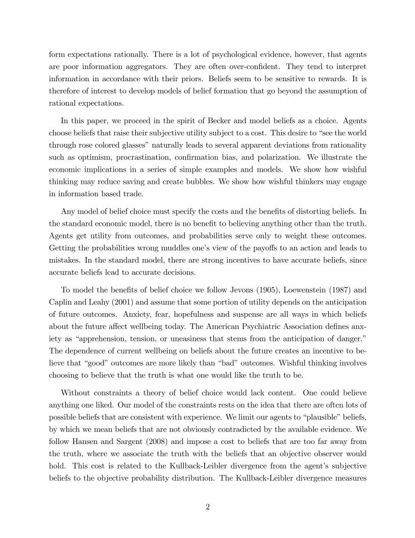
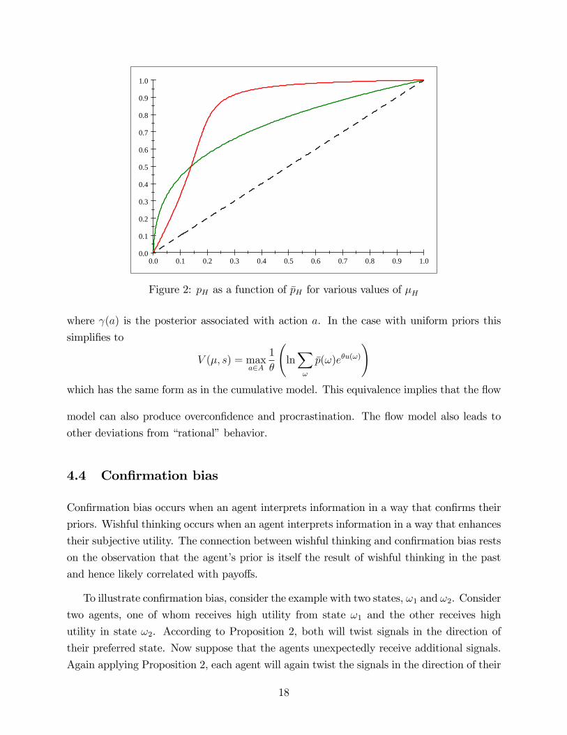
Figure 3 illustrates the effect of the prior on the chosen beliefs. The black line shows pHas a function of pH when the prior is uniform and the parameters are as in Figure 1. The

green line shows the effect of increasing µH to .75. As stated in Proposition 2, the increase

in µH increases pH for low values of pH and reduces pH for high values of pH . The red line

shows that reducing µH to .25 has the opposite effect.

4.3.1 Action Choice

We can calculate the value of the action a under the optimal beliefs (see the appendix).

Substituting (9) into V (µ, s) for a given action choice a yields,

V (µ, s) = maxa∈A

Eγ(a)u(a, ω) +1

θ

(ln∑ω

p(ω)eθ∂Eγ(a)u(ω)

∂p(ω)

)

17

0.0 0.1 0.2 0.3 0.4 0.5 0.6 0.7 0.8 0.9 1.00.0

0.1

0.2

0.3

0.4

0.5

0.6

0.7

0.8

0.9

1.0

Figure 2: pH as a function of pH for various values of µH

where γ(a) is the posterior associated with action a. In the case with uniform priors this

simplifies to

V (µ, s) = maxa∈A

1

θ

(ln∑ω

p(ω)eθu(ω)

)which has the same form as in the cumulative model. This equivalence implies that the flow

model can also produce overconfidence and procrastination. The flow model also leads to

other deviations from “rational”behavior.

4.4 Confirmation bias

Confirmation bias occurs when an agent interprets information in a way that confirms their

priors. Wishful thinking occurs when an agent interprets information in a way that enhances

their subjective utility. The connection between wishful thinking and confirmation bias rests

on the observation that the agent’s prior is itself the result of wishful thinking in the past

and hence likely correlated with payoffs.

To illustrate confirmation bias, consider the example with two states, ω1 and ω2. Consider

two agents, one of whom receives high utility from state ω1 and the other receives high

utility in state ω2. According to Proposition 2, both will twist signals in the direction of

their preferred state. Now suppose that the agents unexpectedly receive additional signals.

Again applying Proposition 2, each agent will again twist the signals in the direction of their

18

preferred state, which will also be the direction of their priors.

Most tests of confirmation bias take the priors as given and evaluate how an agent

interprets additional information. They do not consider the agent’s subjective utility. It is

therefore diffi cult to know whether the interpretation is being influenced by the prior beliefs

or whether both beliefs and the interpretation are being influenced by payoffs. A few studies

attempt to disentangle the effects of beliefs and payoffs. Mijovic-Prelec and Prelec (2010) had

subjects make incentivized predictions before and after being given stakes in the outcomes.

There was a tendency for subjects to reverse their predictions when the state that they had

predicted to be less likely turned out to be the high payoff state. Bastardi, Uhlmann, and

Ross (2011) consider a population of parents with similar priors: all profess to believe that

home care is superior to day care for their children. They differ, however, in their payoffs,

as some have chosen home care for their children, while others have chosen day-care. They

find that the interpretation of evidence aligns with the payoffs rather than the prior. The

parents who had placed their children in day care rated the study supporting day care as

superior, whereas the parents who cared for their children at home did the opposite. In both

of these studies, the interpretation of information appears to be more responsive to payoffs

than priors. This does not imply that priors do not matter, but only that wishful thinking

might be present as well.

4.5 Polarization

Polarization occurs when two agents with opposing beliefs see the same signal and each

becomes more convinced that their view is the correct one. Wishful thinkers can exhibit

polarization if they place different values on the states and the information that they receive

is suffi ciently ambiguous.

Consider a setting with two agents labeled i and j and two states labeled ω1 and ω2.

Suppose that agent i receives utility uH in state ω1 and uL in state ω2 and agent j receives

utility uH in state ω2 and uL in state ω1. In keeping with our discussion of confirmation

bias, suppose that each has received some information in the past that they have interpreted

optimistically, so that agent i has a prior that places weight µH > 12on state ω1, and agent

j places the same prior on state ω2. Each then sees the same signal s which has objective

probability p. Each interprets the signal according to (11). Agent i ends up with the posterior

γi(ω1) =µH p(ω1)

µH p(ω1) + (1− µH)p(ω2)e− θµHµL(uH−uL)(pHµH+pLµL)

2

19

and agent j ends up with the posterior

γj(ω1) =(1− µH)p(ω1)

(1− µH)p(ω1) + µH p(ω2)eθµHµL(uH−uL)(pHµH+pLµL)

2

Polarization occurs if γi(ω1) > µH and γj(ω1) < 1 − µH in which case both agents have

observed the same signal and each has become more confident in their assessment of the

state. Now γi(ω1) > µH ifp(ω2)

p(ω1)e− θµHµL(uH−uL)(pHµH+pLµL)

2 < 1.

Similarly γj(ω1) < 1− µH ifp(ω2)

p(ω1)eθµHµL(uH−uL)(pHµH+pLµL)

2 > 1.

Since exp[− θµHµL(uH−uL)

(pHµH+pLµL)2

]< 1 and exp

[θµHµL(uH−uL)(pHµH+pLµL)2

]> 1, it follows immediately that

polarization is possible, and that polarization is more likely (at least in this example) when

the objective odds p(ω2)p(ω1)

are close to even and when uH − uL is large. In other words,

polarization tends to occur with the signal is relatively uninformative and the desire to

believe is large.

4.6 Comparing the two formulations

The cumulative model and the flow model each have their advantages and disadvantages.

Both approaches can explain overconfidence and procrastination. In addition, the flow model

can explain confirmation bias and polarization. The cumulative model cannot. The reason

is that subjective posteriors are closely tied to objective posteriors in (4). News that raises

γ(ω) will tend to raise γ(ω) for all agents. The cumulative model leads to an algebraically

simpler solution which may prove useful in dynamic applications.

There are other differences in the two approaches. Agents in the flow model are subjective

Bayesians and appear non-Bayesian to an objective observer. On the other hand, agents in

the cumulative model maximize (3). They therefore appear to be objective Bayesians with

an Epstein-Zin utility function. If one attempts to elicit their subjective beliefs, however,

these subjective beliefs will appear non-Bayesian.

Beliefs are more stable in the flow model. They evolve with the flow of information.

Beliefs can potentially change dramatically in the cumulative model. If an agent chooses

action a, and the payoff to action a changes, then the agent will alter their beliefs even if

20

they have not received any new information.

5 Three asset pricing models

In this section we illustrate some of the equilibrium implications of the theory through three

asset pricing models. The first is a model with a risk free bond and idiosyncratic income risk

along the lines of Huggett (1993) extended to include agents that differ in their optimism.

All else equal the more optimistic agents tend to consume more and save less, and therefore

are less wealthy in steady state. The equilibrium interest rate is above that in an economy

without optimism. The second is a model of trade with private information. Again we assume

that agents differ in their optimism. We show that informed traders, whether optimistic or

not, can profit from their private information by trading with agents with different beliefs.

The third model is a model of bubbles in the spirit of Kindleberger. Occasionally optimists

get lucky; their wealth increases; and their influence on asset prices grows, raising asset

prices for a time above what is warranted by objective observers.

5.1 A Huggett economy

Time is discrete. There is a single asset, a risk free bond, with a gross return R. There are

a continuum of agents indexed by i ∈ [0, 1]. Agents indexed by i ∈ [0, η] are objective. They

maximize

E∞∑t=0

βtu(ct)

The remainder of agents are wishful thinkers.

Each period t, each agent i receives an endowment yit. yit takes one of S values y1, . . . yS ≡Y . The realizations of yit follow a Markov chain with transition probabilities pss′ = Pryit =

ys′|yit−1 = s.

The state of individual i in period t is (Ai, yi) where Ai is their in period t−1 saving and

yi is their current-period endowment income. We restrict Ai > φ where φ + y1/(1− β) ≥ 0

so that the agent can always pay off their debts if saving is negative.

We need to extend (3) to a dynamic setting. We construct the dynamic analog of the

cumulative model. We maintain the assumption that wishful thinkers are sophisticated

and that they understand the relationship between action choice and beliefs. Given their

21

initial state (A0, y0), we assume that they choose a sequence of state contingent plans A′(yt)

subjective beliefs γ(yt) where yt is the history of endowment realizations through period t.

Their maximization problem is:

V w(A0, y0) = maxγ(yt)t>0,y∈Y ,A(yt)t>0,y∈Y

∞∑t=0

βt∑y∈Y

γ(yt)u(RA(yt−1(yt)) + yt − A(yt))

−1− βθ

∞∑t=1

βt∑yt∈Y t

γ(yt) lnγ(yt)

γ(yt)

where A > φ and yt−1(yt) denotes the history through yt−1 embedded in the history yt. As

before the first term is subjective expected utility. The second term is the cost of distorting

beliefs. We allow the agent to manipulate beliefs at all horizons. We discount the distortion

of future beliefs at the same rate as future utility. The 1 − β in front compensates for thefact that distorting γ(ys) also tends to distort γ(yt) for all t > s.

If we assume subjective beliefs are consistent in the sense that the conditional expecta-

tions satisfy the laws of probability, γ(yt) = γ(ys(yt))γ(yt|ys(yt)) for all 0 < s < t, then we

can write the cost of distorting yt recursively. For ys = ys(yt),

γ(yt) lnγ(yt)

γ(yt)=

[γ(ys) ln

γ(ys)

γ(ys)+ γ(ys)γ(yt|ys) ln

γ(yt|ys)γ(yt|ys)

]The cost of distorting yt is the cost of distorting ys plus the cost of distorting yt conditional

on ys. This allows us to write the wishful thinker’s problem recursively (see the appendix

for the details):

V w(A, y) = maxA′>φ,γ(y′)y′∈Y

u(c) + β∑y1∈Y

γ(y′)V w(A′, y′)− β

θ

∑y1∈Y

γ(y′) lnγ(y′)

γ(y′)(12)

= maxA′>φ

u(c) +1

θlnE(A,y) expθV w(A′, y′)

where it is understood that c = RA+y−A′ and the second equality comes from substitutingthe optimal beliefs as in (5). Note that choice is dynamically consistent in this setting. Even

though, following Jevons, we think of the agent as choosing the entire future sequence of

beliefs and actions to maximize their current subjective utility, the agent solves a problem of

similar form in the future so that the subjective plans that the agents contemplates in one

period become actual plans when future states are realized.

An equilibrium is an interest rate R, two densities ho(A, y) and hw(A, y), and two func-

22

tions co(A, y) and cw(A, y) such that co(A, y) is the optimal policy of the objective agents

and cw(A, y) is the optimal policy of the wishful thinkers, the goods market clears∫ η

0

co(Ait−1, yit) +

∫ 1

η

cw(Ait−1, yit) =

∫ 1

0

yit

and ho(A, y) and hw(A, y) characterize the steady state distribution across states of the two

types of agent respectively.

We have the following proposition (the proof is in the appendix).

Propostion The following hold:

1. An equilibrium exists.

2. The consumption function cw(A, y) and the value function V w(A, y) for the wishful

thinkers are increasing in both their arguments.

3. Whenever A′ > φ, the Euler equation for the optimists is

u′(cw(A, y)) = βRE(A,y)

[expθV w(A′, y′)

E(A,y) [expθV w(A′, y′)]u′(cw(A′, y′))

].

where E(A,y) is the objective expectation conditional on y.

4. Given y, ho(A, y) first order stochastically dominates hw(A, y).

5. R is decreasing in η.

The first three results follow from standard dynamic programming arguments. Given

that high value states tend to be high consumption states and high consumption states

are low marginal utility states, the Euler equation implies that wishful thinkers tend to

place greater weight on low marginal utility states than do the objective agents. It follows

that E(A,y)u′(cw(A′,y′))u′(cw(A,y))

> E(A,y)u′(co(A′,y′))u′(co(A,y))

whenever A′ > φ, and that wishful thinkers consume

more, save less, and have lower wealth. The lower wealth explains point 4. The precautionary

savings motive of the objective agents tends to push down the real interest rate. Wishful

thinkers’ optimism tends to push the interest rate up. R is therefore increasing in the

proportion of wishful thinkers.

Figure 4 depicts the determination of the equilibrium. The interest rate R is on the

vertical axis. The two curves depict the average saving of each type of agent: Aw(R) for

23

wishful thinkers and Ao(R) for objective agents. These converge to φ as R falls to −∞and Ao(R) converges to ∞ as R reaches 1/β. Since the objective agents save more, Ao(R)

is always to the right of Aw(R). The equilibrium is at the point that total saving in the

economy is equal to zero, so that ηAo(R) + (1− η)Aw(R) = 0.

[Insert Figure 4]

5.2 Information-based trade

In our Huggett economy, agents have access to the same objective information yet hold

different beliefs. The fact that they “agree to disagree”indicates that our model might lie

outside of the class of considered by Milgrom and Stokey (1982). In fact, relative to Milgrom

and Stokey, our model relaxes the assumption that it is common knowledge that all agents

are rational expected utility maximizers.11

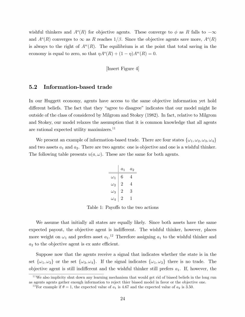
We present an example of information-based trade. There are four states ω1, ω2, ω3, ω4and two assets a1 and a2. There are two agents: one is objective and one is a wishful thinker.

The following table presents u(a, ω). These are the same for both agents.

a1 a2

ω1 6 4

ω2 2 4

ω3 2 3

ω4 2 1

Table 1: Payoffs to the two actions

We assume that initially all states are equally likely. Since both assets have the same

expected payout, the objective agent is indifferent. The wishful thinker, however, places

more weight on ω1 and prefers asset a1.12 Therefore assigning a1 to the wishful thinker and

a2 to the objective agent is ex ante effi cient.

Suppose now that the agents receive a signal that indicates whether the state is in the

set ω1, ω2 or the set ω3, ω4. If the signal indicates ω1, ω2 there is no trade. Theobjective agent is still indifferent and the wishful thinker still prefers a1. If, however, the

11We also implicity shut down any learning mechanism that would get rid of biased beliefs in the long runas agents agents gather enough information to reject thier biased model in favor or the objective one.12For example if θ = 1, the expected value of a1 is 4.67 and the expected value of a2 is 3.50.

24

signal indicates ω3, ω4. the objective agent remains indifferent, but the wishful thinkerplaces greater weigh on ω3 and prefers to trade a1 for a2. The objective agent obliges.

Note that the signal could be the private information of the wishful thinker without

affecting this outcome. The wishful thinker’s willingness to trade would reveal that their

information set is ω3, ω4, but the agents would agree to disagree on the relative probabilitiesof ω3 and ω4 and trade would still take place. Similarly we could raise the payoffto a1 in state

ω3 and the payoff to a2 in state ω2 by a small amount ε without altering the ex ante effi ciency

of the allocation, and then the signal could be the private information of the objective agent

and trade would take place in the case that the signal was ω3, ω4.

In this example, agents learn from trade and still retain different beliefs. This differen-

tiates our framework from other models of trade with heterogeneous beliefs in which agents

do not learn from trade such as Blume and Easley (1992), Geanakoplos (2003), Borovicka

(2018), or Caballero and Simsek (2018).

5.3 Bubbles

We saw in our Huggett economy that the presence of wishful thinkers can drive up the price

of an asset, in this case a risk free bond, relative to that of an economy populated only by

objective agents. Here we use this observation to flesh out a story of asset bubbles. In normal

times, assets will be priced mainly by the objective agents as we saw in our Huggett economy

that the wishful thinkers will tend to have less wealth. Every now and then, however, the

wishful thinkers may take over and an asset price may rise above fundamental value, where

fundamental value is taken to be the price in an economy dominated by objective agents.

Kindelberger (1978) describes the typical bubble as follows. The bubble begins with the

introduction of a new asset, typically reflecting a new technology such as railroads, canals,

or information technology. A period of good news then increases interest in the new asset.

In the second phase, interest evolves into euphoria, and prices rise above what would be

expected by an objective observer. This is the bubble phase. Typically the bubble does not

crash immediately. There is a period of hesitation at the top of the market. This is the third

phase. The final phase is the crash, as reality sets in and prices return to normal.

A model with wishful thinkers and objective agents can fit this general pattern. Consider

the introduction of a new technology. Suppose that initially it is not known weather the

technology is viable or not, and that conditional on being viable there is a chance that the

technology is transformative and a chance that the technology is merely mildly profitable.

25

Wishful thinkers will be drawn to the new technology both because it is unproven and hence

uncertain and because it promises high returns. Initially wishful thinkers will make up only a

small portion of the demand for the asset because they tend to be less wealthy than objective

agents. The initial success of the asset may cause their role to grow with time. This happens

for two reasons. First, since the wishful thinkers will hold a greater share of the new asset in

their portfolios, initial reports that the technology is viable will disproportionately benefit

them.13 Second, in the flow model each bit of good news will be interpreted in a positive

light, leading to greater and greater optimism. As the importance of the wishful thinkers

grows, price rises above fundamentals. As the price rises the importance of the wishful

thinkers continues to grow, as objective agents see the market as overvalued. At the top of

the market, when an objective observer would question the potential of the technology to

be transformative, wishful thinkers will tend to downplay bad news. This is the period of

hesitation. Wishful thinking, however, is not magical thinking. Eventually even optimists

must admit that the asset is only mildly successful.

6 Discussion

6.1 Sophistication vs naïveté

We have chosen to model sophisticated agents that are aware of how choices affect their

beliefs. When choosing an action in the decision problems (3) or (12), the agent foresees

that their beliefs will change and takes this into consideration. Another possibility is that

agents are naïve. They may not consider or may not be aware of how their choices affect

their beliefs.

Most of the phenomenon considered above would still be apparent if the agent were naïve.

Optimism, overconfidence and polarization only depended on the choice of beliefs, not on the

choice of actions. Naïveté, however, gives rise to additional phenomenon which we consider

below. Naïveté also gives rise to dynamic inconsistency, as the agent fails to anticipate how

a choice today will affect beliefs that affect choices tomorrow.

Consider a naïve agent in the cumulative model. The agent would not consider how

their choices affect their beliefs, but after making a choice, the agent would choose beliefs

consistent with that choice. This gives rise to the endowment effect, the idea that the mere

13This effect is also present in Caballero and Simsek (2018). The price of the risky asset rises with thewealth of their optimistic agents.

26

possession of an object increases its value (Kahneman, Knetsch, and Thaler, 1990). This

explanation of the endowment effect is similar to those in cognitive science which emphasize

biased search, memory and information processing (See Morewedge and Giblin (2015) for a

review). Since the agent in the flow model manipulates the flow of information and not the

stock of information, the flow model can only explain the endowment effect if the person

who receives the object also receives a signal that they can manipulate.

The “foot-in-the-door technique”involves getting a person to make a big decision by first

having them make a similar decision on a smaller scale (Freedman and Fraser, 1966). As an

example consider a world with two states ωH and ωL. Suppose ωH is more likely, µH > µL.

Consider a gamble in which the agent gets x if the state is ωH and −x otherwise. Supposethat utility, u(x), is increasing and concave. Then it is possible that the agent would choose

the gamble for small x and avoid the gamble for larger x. It is also possible that upon

choosing the gamble for small x, the agent’s posterior γH would rise enough that the agent

would now be willing to take the larger gamble.

6.2 Robustness or Wishful Thinking

Hansen and Sargent (2008) model agents as pessimistic. Their agents are concerned that

their model of the economy is inaccurate, and seek to make sure that their decisions are

robust to plausible alternatives. This leads to an optimization problem very similar to (3),

but the cost (2) enters with the opposite sign and the agent first minimizes with respect

to beliefs before maximizing with respect to actions. Not surprisingly, this leads to very

different behavior. The agent distorts beliefs toward the low payoff states instead of the high

payoff states, and behaves as if they have a preference for early resolution of uncertainty

rather than late resolution of uncertainty.

Which model is a better is a better model of human behavior is not an easy question

to answer. Each model is supported by its own body of psychological evidence and each

performs well on in certain domains and poorly in others. The psychological justification

for robustness is that it is consistent with ambiguity aversion and generates a preference

for late resolution of uncertainty, which many find plausible. The economic justification for

robustness is that a preference for robustness gives rise to risk sensitive preferences which

help to explain the behavior of asset prices, in particular the equity premium.

As discussed above, there is also psychological evidence that agents distort beliefs in

the direction of payoffs, and the psychological evidence in favor of optimism is at least

27

as strong as that in favor of ambiguity. While robustness appears to help explain asset

pricing behavior, there are many economic situations where are better explained by wishful

thinking. Entrepreneurs, for example, appear optimistic. To quote Daniel Kahneman, “A lot

of progress in the world is driven by the delusional optimism of some people.”Cooper, Woo,

and Dunkelburg (1988) find that two thirds of entrepreneurs believe that their firm will fare

better than similar firms run by others. Hamilton (2000) finds that the median earnings of

entrepreneurs is 35% less than would they would be predicted to earn in alternative jobs. Hall

and Woodward (2010) argue that due to the extreme dispersion in payoffs, an entrepreneur

backed by venture capital with rational expectations and a coeffi cient of relative risk aversion

equal to two should place a certainty equivalent value only slightly greater than zero on the

distribution of outcomes that they face at the time that they start their company. Dropping

out of Harvard to develop a social networking site as Mark Zuckerberg did would appear

much more consistent with optimism than a preference for robustness.

Many self-control problems would would appear to be more consistent with optimism

than robustness. We have already cited the evidence on gym memberships (DellaVigna and

Malmendier, 2006). Payday lending is another example. Payday loans typically accrue about

18% over a period of two weeks or an annualized value of over 7000%. Borrowers appear

to be overoptimistic regarding their ability to repay and end up rolling loans over multiple

times. Borrowers also tend to be optimistic regarding how many times they will roll over

debt.

It is a question for future research to find the key determinants of when a domain is more

appropriate for wishful thinking and when a domain is more appropriate for robustness. Our

Huggett economy suggests that in normal times asset pricing may naturally be a domain

for robustness, since wishful thinkers tend to accumulate less wealth. Our discussion of

bubbles suggests that sometimes, however, wishful thinkers may come to play a larger role.

Entrepreneurship, on the other hand, would seem to be a natural domain for wishful thinking.

It may also be the case that the same agents are wishful thinkers in some situations and

robust in others. Bassanin, Faia, and Valaria (2018) take a step in this direction. Citing

psychological research that suggests people are sometimes ambiguity averse and sometimes

ambiguity seeking and that these attitudes are state dependent, they construct a business

cycle model that incorporates both behaviors. They assume that agents are ambiguity averse

if the value function is below its historical mean, and ambiguity seeking otherwise. Their

model amplifies business cycles by generating optimism in booms and pessimism in busts.

28

6.3 Brunnermeier and Parker

The most closely related paper is Brunnermeier and Parker (2005). That paper like our

paper presents a model of belief choice in which the benefit of belief choice is that beliefs

enter directly into utility. Like our agents in the flow model, their agents are subjective

Bayesians. Their model leads to many of the same phenomenon as our model, in particular

optimism and overconfidence.

There are, however, several differences. First, the two papers model the costs of belief

choice in very different ways. Brunnermeier and Parker focus on how optimistic beliefs

might lead to suboptimal decisions. In their model there is an initial period in which the

agent chooses their prior. In subsequent periods, the agent observes the world, updates their

information as would a Bayesian and makes decisions. The period-zero agent balances the

utility gain from choosing an optimistic prior against the against the mistakes that result

from this mistaken prior. The period-zero agent uses the objective probabilities to weight

outcomes. Our agents do not consider the costs that arise from mistaken beliefs. Instead we

place the cost in how far their beliefs deviate from the objective evidence.

Second, while agents in both models may be subjective Bayesians, they deviate from

objective Bayesians in very different ways. In Brunnermeier and Parker, agents have an

incorrect prior, but their interpretation of evidence accords with objective reality. In our

flow model, agents may or may not have an incorrect prior, it is there interpretation of

signals that is overly optimistic.

Finally, agents in the Brunnermeier and Parker model make a once and for all choice of

beliefs. All belief choice occurs in the initial period. Our agents twist beliefs at every point

in their life, and in particular when they make choices. In Brunnermeier and Parker the

initial choice of beliefs tends to affect future choices. In our model, past choices also mold

future beliefs.

7 Conclusion

Wemodel an agent who gets utility from their beliefs and therefore interprets information op-

timistically. The framework can explain behavioral biases such as optimism, procrastination,

confirmation bias, polarization, the endowment effect, and the foot-in-the-door phenomenon.

In spite of these biases, the agent is subjectively Bayesian in some formulations.

29

Our theory is based on two fundamental ideas. First that agents derive utility from their

beliefs along the lines of Jevons (1905), Loewenstein (1987) and Caplin and Leahy (2001).

The second is that at any point in time there are a set of models of the world that are all

plausible (Hansen and Sargent, 2008), so that agents have some freedom in choosing their

beliefs without choosing beliefs that are obviously wrong.

An interesting direction for future research is to endogenize the set of plausible models.

This could be done either on the supply side or the demand side. If one takes the view

that the set of plausible models is well represented by the views in the mainstream media,

one could endogenize this supply along the lines Mullainathan and Schlifer (2005). On the

demand side, one could imagine enriching the model to add a choice of attention along the

lines of Sims (1998), Matejka and McKay (2015), or Caplin, Csaba, Leahy and Nov (2018).

Since wishful thinkers have a preference for late resolution of uncertainty, one might expect

wishful thinkers to exhibit willful ignorance.

30

References

Akerlof, George, and William Dickens (1982), “The Economic Consequences of Cognitive

Dissonance,”American Economic Review, 72, 307-319.

Aiyagari, Rao (1994), “Uninsured Idiosyncratic Risk and Aggregate Saving,”Quarterly Jour-

nal of Economics 109, 659-646.

Bassanin, Marzio, Esterh Faia, and Valeria Patella (2018), “Ambiguous Leverage Cycles,”

working paper.

Bastardi, A.; Uhlmann, E. L.; Ross, L. (2011), “Wishful Thinking: Belief, Desire, and the

Motivated Evaluation of Scientific Evidence,”Psychological Science, 22, 731—732.

Benabou, Roland, and Jean Tirole (2002), “Self-Confidence and Personal Motivation,”Quar-

terly Journal of Economics 117, 871-915.

Benabou, Roland, and Jean Tirole (2016), “Mindful Economics: The Production, Consump-

tion, and Value of Beliefs,”Journal of Economic Perspectives 30, 141-164.

Bernardo, Antonio, and Ivo Welch (2001), “On the Evolution of Overconfidence and Entre-

preneurs,”Journal of Economics and Management Strategy, 10, 301-330.

Blume, Lawrence, and David Easley(1992), “Evolution and Market Behavior.” Journal of

Economic Theory 58, 9—40.

Brunnermeier, Markus and Jonathan Parker (2005), “Optimal Expectations,” American

Economic Review, 1092-1118.

Burnside, Craig, Martin Eichenbaum and Sergio Rebelo (2016), “Understanding Housing

Booms and Busts,”Journal of Political Economy 124, 1088-1147.

Bordalo, Pedro, Nicola Gennaioli, and Andrei Schleifer (2018), “Diagnostic Expectations

and Credit Cycles," Journal of Finance 73, 199-227.

Borovicka, Jaroslav (2018), “Survival and Long-Run Dynamics with Heterogeneous Beliefs

under Recursive Preferences,”Journal of Political Economy, forthcoming.

Caballero, Ricardo, and Alp Simsek (2108), “A Risk-centric Model of Demand Recessions

and Macroprudential Policy,”NBER Working Paper No. 23614

Caplin, Andrew, and John Leahy (2001), “Psychological Expected Utility,”Quarterly Jour-

nal of Economics 116, 55—79.

31

Caplin, Andrew, and John Leahy (2004), “The Supply of Information by a Concerned Ex-

pert,”Economic Journal 114, 487-505.

Caplin, Andrew, and John Leahy (2006), “The Social Discount Rate,”Journal of Political

Economy 112, 1257-1268.

Caplin, Andrew, Daniel Csaba, John Leahy, and Oded Nov (2018), “Rational Inattention

and Psychometrics,”working paper.

Cooper, Arnold, Carolyn Woo, and William Dunkelburg (1988), “Entrepreneur’s Perceived

Chances of Success,”Journal of Business Venturing 3, 97-108.

Dixit, Avinash (1989), “Entry and Exit Decisions under Uncertainty,”Journal of Political

Economy 97, 620-638.

Debondt, Werner, and Richard Thaler (1996), “Financial Decision Making in Markets and

Firms: A Behavioral Perspective,” Handbook in Operations Research and Management

Science 9, North-Holland.

DellaVigna Stefano, and Ulrike Malmendier (2006), “Paying not to go to the Gym,”Amer-

ican Economic Review 96, 694-719.

Epstein, Larry, and Stanley Zin (1989), “Substitution, Risk Aversion, and the Temporal

Behavior of Consumption and Asset Returns: A Theoretical Framework,”Econometrica, 57,

937-969.

Freedman, J. L., and S. C. Fraser (1966), “Compliance without pressure: The foot-in-the-

door technique.”Journal of Personality and Social Psychology 4, 195—202.

Fuster, Andreas, David Laibson, and Brock Mendel (2012), “Natural Expectations and Eco-

nomic Fluctuations," Journal of Economic Perspectives 24, 87-84.

Gabaix, Xavier (2014), “A Sparsity-Based Model of Bounded Rationality,”Quarterly Journal

of Economics 129, 1661-1710.

Geanakoplos, John (2003) “Liquidity, Default, and Crashes: Endogenous Contracts in Gen-

eral Equilibrium,”in Advances in Economics and Econometrics: Theory and Applications,

Econometric Society Monographs, Eighth World Conference 2, 170—205. New York: Cam-

bridge University Press.

Hall, Robert, and Susan Woodward (2010), “The Burden of the Nondiversifiable Risk of

Entrepreneurship,”American Economic Review 100, 1163-1194.

32

Hamilton, Barton (2000), “Does Entrepreneurship Pay? An Empirical Analysis of the Re-

turns to Self-employment,”Journal of Political Economy 103, 604-631.

Hansen, Lars, and Thomas Sargent (2008), Robustness, Princeton: Princeton University

Press.

Hopenhayn, Hugo (1992), “Entry, Exit, and Firm Dynamics in Long Run Equilibrium,”

Econometrica 60, 1127-1150.

Huggett, Mark (1993), “The Risk Free Rate in Heterogeneous-Agent, Incomplete-Insurance

Economies,”Journal of Economic, Dynamics and Control 17, 953-969.

Jevons, William (1905), Essays in Economics, London: Macmillan.

Kahneman, Daniel, Jack Knetsch, and Richard Thaler (1990), “Experimental Tests of the

Endowment Effect and the Coase Theorem,”Journal of Political Economy 98, 1325—1348.

Kindelberger, Charles (1978), Manias, Crashes and Panics, New York: Basic Books.

Knox, R. E., Inkster, J. A. (1968), “Postdecision Dissonance at Posttime,”Journal of Per-

sonality and Social Psychology, 18, 319—323.

Lord, Charles, Lee Ross and Mark Lepper (1979), “Biased Assimilation and Attitudinal

Polarization: The Effects of Prior Theories on Subsequently Considered Evidence,”Journal

of Personality and Social Psychology, 37, 2098-2109.

Loewenstein, George (1987), “Anticipation and the Valuation of Delayed Consumption,”

The Economic Journal, 97, 666—684.

Milgrom, Paul, and Nancy Stokey (1982), “Information, Trade, and Common Knowledge,”

Journal of Economic Theory 26, 17-27.

Mijovic-Prelec, Canica, and Drazen Prelec (2010), “Self-Deception as Self-Signalling: A

model and Experimental Evidence,” Philosophical Transactions of the Royal Society, B,

265, 227-240.

Morewedge, Carey, and Colleen Giblin (2015), “Explanations of the endowment effect: an

integrative review,”Trends in Cognitive Sciences 19, 339—348.

Matejka, Filip, and Alisdair McKay (2015), “Rational Inattention to Discrete Choices: A

New Foundation for the Multinomial Logit Model,”American Economic Review, 105, 272-

298.

Mullainathan, Sendil, and Andrei Schlifer (2005), “The Market for News,”American Eco-

33

nomic Review 95, 1031-1052.

Sims, Christopher (1998), “Stickiness,”Carnegie-Rochester Conference Series on Public Pol-

icy 49, :317-356.

34

8 Appendix

8.1 Derivation of (9)

Consider the maximization problem (3) for fixed a ∈ A. The first order condition for p(ω) is

0 =µ(ω)u(ω)∑ω′ p(ω

′)µ(ω′)−∑ω′

p(ω′)µ(ω′)µ(ω)u(ω′)

[∑

ω′′ p(ω′′)µ(ω′′)]2

− 1

θln

p(ω)

p∗(ω)− 1

θ− λ

where λ is the Lagrange multiplier on the constraint∑

ω p(ω) = 1. We ignore the constraint

p(ω) ≥ 0. We will show that the it is never binding.

Solving for p(ω),

p(ω) = p(ω) exp

[θ

µ(ω)u(ω)∑ω′ p(ω

′)µ(ω′)− θ

∑ω′

p(ω′)µ(ω′)µ(ω)u(ω′)

[∑

ω′′ p(ω′′)µ(ω′′)]2

− 1− θλ]

(13)

Summing over ω implies,

1 =∑ω

p(ω) =∑ω

p(ω) exp

[θ

µ(ω)u(ω)∑ω′ p(ω

′)µ(ω′)− θ

∑ω′

p(ω′)µ(ω′)µ(ω)u(ω′)

[∑

ω′′ p(ω′′)µ(ω′′)]2

− 1− θλ](14)

Dividing the left-hand side of (13) by the left-hand side of (14) yields,

p(ω) =

p(ω) exp

[θ µ(ω)u(ω)∑

ω′ p(ω′)µ(ω′) − θ

∑ω′

p(ω′)µ(ω′)µ(ω)u(ω′)

[∑ω′′ p(ω

′′)µ(ω′′)]2

]∑

ω′ p(ω) exp

[θ µ(ω′)u(ω′)∑

ω′′ p(ω′′)µ(ω′′) − θ

∑ω′′

p(ω′′)µ(ω′′)µ(ω′)u(ω′′)

[∑ω′′′ p(ω

′′′)µ(ω′′′)]2

]Note that the e−1−θλ terms drop out.

To complete the derivation note,

∂Eγu(ω)

∂p(ω)=

µ(ω)u(ω)∑ω′ p(ω

′)µ(ω′)−∑ω′

p(ω′)µ(ω′)µ(ω)u(ω′)

[∑

ω′′ p(ω′′)µ(ω′′)]2

where Eγ is the expectation with respect to γ. Also note that given p ∈int∆(Ω), p ∈int∆(Ω)

so the constraint p(ω) ≥ 0 is never binding.

35

8.2 Derivation of the Value of action a

Substituting (9) into (8)

∑ω

p(ω)µ(ω)∑ω′ p(ω

′)µ(ω′)u(ω)− 1

θ

∑ω

p(ω) lnp(ω)

p(ω)

=∑ω

p(ω) exp[θ∂Eγu(ω)

∂p(ω)

]∑ω′ p(ω

′) exp[θ∂Eγu(ω′)∂p(ω′)

]µ(ω)

∑ω′

p(ω′) exp[θ∂Eγu(ω′)∂p(ω′)

]∑ω′′ p(ω

′′) exp[θ∂Eγu(ω′′)∂p(ω′′)

]µ(ω′)

u(ω)− 1

θ

∑ω

p(ω) exp[θ ∂Eγu(ω)

∂p(ω)

]∑

ω′ p(ω′) exp

[θ ∂Eγu(ω′)

∂p(ω′)

] ln

p(ω) exp[θ∂Eγu(ω)

∂p(ω)

]∑ω′ p(ω

′) exp[θ∂Eγu(ω′)∂p(ω′)

]p(ω)

=

∑ω p(ω) exp

[θ ∂Eγu(ω)

∂p(ω)

]µ(ω)u(ω)∑

ω′ p(ω′) exp

[θ ∂Eγu(ω′)

∂p(ω′)

]µ(ω′)

− 1

θ

∑ω p(ω) exp

[θ ∂Eγu(ω)

∂p(ω)

]∑

ω′ p(ω′) exp

[θ ∂Eγu(ω′)

∂p(ω′)

] lnexp

[θ ∂Eγu(ω)

∂p(ω)

]∑

ω′ p(ω′) exp

[θ ∂Eγu(ω′)

∂p(ω′)

]=

∑ω p(ω) exp

[θ ∂Eγu(ω)

∂p(ω)

]µ(ω)u(ω)∑

ω′ p(ω′) exp

[θ ∂Eγu(ω′)

∂p(ω′)

]µ(ω′)

−

∑ω p(ω) exp

[θ ∂Eγu(ω)

∂p(ω)

]∂Eγu(ω)

∂p(ω)∑ω′ p(ω

′) exp[θ ∂Eγu(ω′)

∂p(ω′)

] +1

θln∑ω′

p(ω′) exp

[θ∂Eγu(ω′)

∂p(ω′)

]

Focus on the term ∑ω p(ω) exp

[θ ∂Eγu(ω)

∂p(ω)

]∂Eγu(ω)

∂p(ω)∑ω′ p(ω

′) exp[θ ∂Eγu(ω)

∂p(ω′)

]=

∑ω

p(ω)

(µ(ω)∑

ω′ µ(ω′)p(ω′)(u(ω)− Eγu(ω))

)=

∑ω

(p(ω)µ(ω)∑ω′ µ(ω′)p(ω′)

(u(ω)− Eγu(ω))

)= 0

which completes the derivation.

8.3 Derivation of (12)

We begin with the maximization problem

36

V (A, y) = maxγ(yt)t>0,y∈Y ,A(yt)t>0,y∈Y

∞∑t=0

βt∑y∈Y

γ(yt)u(RA(yt−1(yt)) + yt − A(yt))

−1− βθ

∞∑t=1

βt∑yt∈Y t

γ(yt) lnγ(yt)

γ(yt)

where yt−1(yt) denotes the history through yt−1 embedded in yt and A > 0. The key

observation that allows us to write the problem recursively is that

∑yt∈Y t

γ(yt) lnγ(yt)

γ(yt)=

∑y1∈Y

∑yt s.t. y1∈Y t

γ(y1)γ(yt|y1) ln

(γ(y1)γ(yt|y1)

γ(y1)γ(yt|y1)

)

=∑y1∈Y

γ(y1) lnγ(y1)

γ(y1)+

∑yt s.t. y1∈Y t

γ(y1)γ(yt|y1) lnγ(yt|y1)

γ(yt|y1)

so that

1

θ(1− β)

∞∑t=0

βt∑yt∈Y t

γ(yt) lnγ(yt)

γ(yt)

=1

θ(1− β)

∞∑t=1

βt∑y1∈Y

γ(y1) lnγ(y1)

γ(y1)+

∑yt s.t. y1∈Y t

γ(y1)γ(yt|y1) lnγ(yt|y1)

γ(yt|y1)

=

1

θ(1− β)

∞∑t=1

βt∑y1∈Y

γ(y1) lnγ(y1)

γ(y1)+

∑yt s.t. y1∈Y t

γ(y1)γ(yt|y1) lnγ(yt|y1)

γ(yt|y1)

=β

θ

∑y1∈Y

γ(y1) lnγ(y1)

γ(y1)+∑y1∈Y

βγ(y1)1− βθ

∞∑t=2

βt−1

∑yt s.t. y1∈Y t

γ(yt|y1) lnγ(yt|y1)

γ(yt|y1)

Similarly we can rewrite expected utility

∞∑t=0

βt∑y∈Y

γ(yt)u(RA(yt)− A(yt−1(yt)))

= u(RA(y1)− A0) +

∞∑t=1

ββt−1∑y1∈Y

∑yt s.t. y1∈Y t

γ(y1)γ(yt|y1)u(RA(yt)− A(yt−1(yt)))

= u(RA(y1)− A0) + β∑y1∈Y

γ(y1)∞∑t=1

βt−1∑

yt s.t. y1∈Y tγ(yt|y1)u(RA(yt)− A(yt−1(yt)))

37

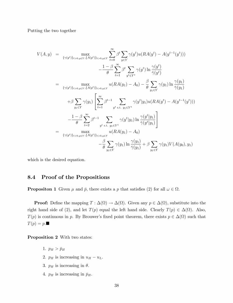
Putting the two together

V (A, y) = maxγ(yt)t>0,y∈Y ,A(yt)t>0,y∈Y

∞∑t=0

βt∑y∈Y

γ(yt)u(RA(yt)− A(yt−1(yt)))

−1− βθ

∞∑t=1

βt∑yt∈Y t

γ(yt) lnγ(yt)

γ(yt)

= maxγ(yt)t>0,y∈Y ,A(yt)t>0,y∈Y

u(RA(y1)− A0)− β

θ

∑y1∈Y

γ(y1) lnγ(y1)

γ(y1)

+β∑y1∈Y

γ(y1)

∞∑t=1

βt−1∑

yt s.t. y1∈Y tγ(yt|y1)u(RA(yt)− A(yt−1(yt)))

−1− βθ

∞∑t=2

βt−1∑

yt s.t. y1∈Y tγ(yt|y1) ln

γ(yt|y1)

γ(yt|y1)

= max

γ(yt)t>0,y∈Y ,A(yt)t>0,y∈Yu(RA(y1)− A0)

−βθ

∑y1∈Y

γ(y1) lnγ(y1)

γ(y1)+ β

∑y1∈Y

γ(y1)V (A(y0), y1)

which is the desired equation.

8.4 Proof of the Propositions

Propositon 1 Given µ and p, there exists a p that satisfies (2) for all ω ∈ Ω.

Proof: Define the mapping T : ∆(Ω)→ ∆(Ω). Given any p ∈ ∆(Ω), substitute into the

right hand side of (2), and let T (p) equal the left hand side. Clearly T (p) ∈ ∆(Ω). Also,

T (p) is continuous in p. By Brouwer’s fixed point theorem, there exists p ∈ ∆(Ω) such that

T (p) = p.

Proposition 2 With two states:

1. pH > pH

2. pH is increasing in uH − uL.

3. pH is increasing in θ.

4. pH is increasing in pH .

38

5. There exists µ such that pH is increasing in µH for µH < µ and decreasing in µHfor µH > µ.

Proof (Sketch): At any solution

pH =pH

pH + pLe− θµHµL(uH−uL)(pHµH+pLµL)

2

(1) follows from the observation that uH > uL implies e− θµHµL(uH−uL)(pHµH+pLµL)

2 < 1.

Consider now T mapping defined in Proposition 1 and applied to the example with two

states.

T (pH) =pH

pH + pLe− θµHµL(uH−uL)(pHµH+pLµL)

2

Note that when pH = 0, we have

T (0) =pH

pH + pLe− θµH

µL(uH−uL)

> 0

and when pH = 1

T (1) =pH

pH + pLe− θµLµH

(uH−uL)< 1

Now consider the derivative of the value function

pHµHuH + pLµLuLpHµH + pLµL

− 1

θpH ln pH/pH −

1

θpL ln pL/pL

which is

µHuH − µLuLpHµH + pLµL

− pHµHuH + pLµLuL(pHµH + pLµL)2

(µH − µL)− 1

θln pH/pH +

1

θln(1− pH)/pL

Note that this is positive and infinite if pH = 0 or 1. Hence the first and last critical points

are maxima. Generically every local maximum is associated with a point T (p) = p such that

T ′(p) < 1.

(2), (3) and (4) follow from the observation that T is increasing in µH − µL, θ, and pHtogether with the observation that T ′(p) < 1 at all maxima.

Consider the effect of an increase in µH onµHµL

(pHµH+pLµL)2= µH(1−µH)

(pHµH+pL(1−µH))2the derivative

39

is1− 2µH

(pHµH + pLµL)2− 2

(µH − µ2H)(pH − pL)

(pHµH + pLµL)3

This has the same sign as

(1− 2µH)(pHµH + pLµL)− 2(µH − µ2H)(pH − pL) = 1− µH − pH

So µH(1−µH)(pHµH+pL(1−µH))2

is increasing in µH when µH < 1 − pH and decreasing otherwise. It

follows that T (p) is increasing in µH when µH < 1 − pH and decreasing otherwise, which

implies (4).

Proposition 3 With two states:

1. If µH > µL, then there is only one solution to (11).

2. Given µ and s, there exists θ such that there is only one solution to (11).

Proof (sketch): There can be solution to (11) if the value function is strictly concave.the derivative of the value function is:

dV

dpH=

µHµL(pHµH + pLµ)2

[uH − uL]− 1

θln pH/pH +

1

θln pL/pL

The second derivative is

d2V

dp2H

= −2µHµL(µH − µL)(uH − uL)

(pHµH + pLµL)3− 1

θ

1

pHpL

This is negative if µH > µL, which establishes (1). The first term is continuous in pH on the

interval [0, 1], and is therefore bounded. We can therefore choose, θ small enough that the

expression is negative, which establishes (2).

Proposition 4 The following hold

1. An equilibrium exists.

2. The consumption function cw(A, y) and the value function V w(A, y) for the optimists

are increasing in both their arguments.

3. Whenever A′ > φ, the Euler equation for the wishful thinkers is

u′(cw(A, y)) = βRE(A,y)

[expθV w(A′, y′)

E(A,y) [expθV w(A′, y′)]u′(cw(A′, y′))

].

40

where Ey is the objective expectation conditional on y and V w is the value of an optimal

policy.

4. Given y, ho(A, y) first order stochastically dominates hw(A, y).

5. R is decreasing in η.

Proof (sketch): The Bellman equation for the objective individuals is

V o(A, y) = maxA′>A

u(RA+ y − A′) + βEyVo(A′, y′)

Given R < 1/β, Standard dynamic programming arguments insure that a solution exists.

The Bellman equation for the wishful thinkers is

V w(A, y) = maxA′>A

u(RA+ y − A′) + β lnE expV w(A′, y′)

Note that

maxA′∈A

u(RA+y−A′)+β lnE expV w(A′, y′)+a = maxA′∈A

u(RA+y−A′)+β(E expV wA′, y′))+βa

so that standard dynamic programming arguments apply in this case as well.

The solution defines the policy functions co(A, y;R) and cw(A, y;R). Given co(A, y;R)

and cw(A, y;R) can solve for ho(A, y;R) and hw(A, y;R) and hence EAo(R) and EAw(R).

Note if R = 0, then EAo(R) = EAw(R) = φ. Show that cw(A, y;R) ≥ co(A, y;R). Show

implies ho(A, y;R) dominates hw(A, y;R) and that EAn(R) ≥ EAw(R). Show continuity in

R. This establishes points 1, 2 and 4. Note that this is very much like a two country version

of the Huggett model, we are looking for an R such that EAn(R) + EAw(R) = 0.

We now turn to the Euler equation. First order condition for A′ is

u(RA+ y − A′) = βE expV (A′, y′)V1(A′, y; )

E expV (A′, y′)

The derivative of the value function with respect to A is

d

dAV w(A, y) = R

41

Together these imply.

u(RA+ y − A′) = βRE expV w(A′, y′)u′(c′)E expV w(A′, y′)

This establishes point 3.

Consider R as a function of η, the fraction of objective agents. An increase in η, given

R, drives up consumption and down the interest rate. This establishes point 5.

42

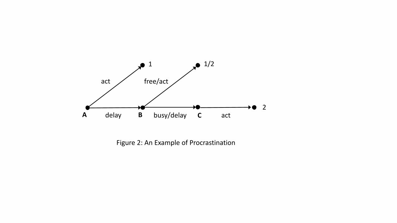
act

delay

free/act

busy/delay act

1 1/2

2A B C

Figure 2: An Example of Procrastination

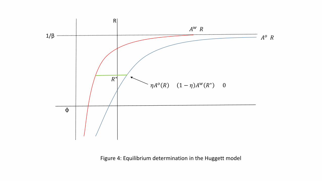
R

1/β 𝐴𝐴𝑜𝑜(𝑅𝑅)

φ

𝐴𝐴𝑤𝑤(𝑅𝑅)

𝜂𝜂𝐴𝐴𝑜𝑜 𝑅𝑅 + 1 − 𝜂𝜂 𝐴𝐴𝑤𝑤 𝑅𝑅∗ = 0𝑅𝑅∗

Figure 4: Equilibrium determination in the Huggett model