WORKING TOGETHER TO DELIVER MORE SUSTAINABLE PRODUCTS ...awsassets.wwfindia.org/downloads/wwf___cotton_carbon_emission.pdf · TOGETHER TO DELIVER MORE SUSTAINABLE PRODUCTS ... .3

WORKINGTOGETHER TODELIVER MORE SUSTAINABLE PRODUCTS

Cutting cotton carbon emissions ~ Findings from Warangal, India

2013REPORT

This report is part of the Marks & Spencer funded project Greenhouse-gas emissions from cotton farms in Warangal district of Andhra Pradesh and is supported by WWF-UK.

This report was prepared by WWF-India. The project team includes WWF- India and WWF-UK.

WWF-India teamSumit RoyMurli DharP Vamshi Krishna

WWF-UK teamRebecca May

EditorsBaya AgarwalBarney Jeffries

ReviewersCool Farm InstituteWWF-UK team

Acknowledgements:The authors acknowledge Professor Jon Hillier, University of Aberdeen for his valuable contribution to developing and modifying the Cool Farm Tool; Daniella Malin, Jessica Mullan and Stephanie Daniels who were based at the Sustainable Food Lab, USA for helping in analysing the data from the Cool Farm Tool; Carmel McQuaid of Marks & Spencer for her constant support to the project; Christof Walter of Unilever for supporting the project and hosting several meetings on the Cool Farm Tool; and Dave Tickner, Megan Chamberlain and Emma Scott from WWF-UK for their support and input.

Cutting cotton carbon emissions~Finding from Warangal, India

Abbreviations

AP : Andhra Pradesh

BMPs : Better management practices

oC : Degree centigrade

CAGR : Compounded annual growth rate

CDP : Carbon Disclosure Project

CH4 : Methane

CO2e : Carbon dioxide equivalent

DAP : Diammoniumphosphate

GDP : Gross domestic product

GHG : Greenhouse gas

GRI : Global Reporting Initiative

Ha : Hectares

HP : Horse power

H&M : Hennes & Mauritz

Kg : Kilograms

MoP : Muraite of Potash (potassium chloride)

MP : Madhya Pradesh

MT : Metric tonnes

MTI : Market Transformation Initiative

M&S : Marks & Spencer

N : Nitrogen

NAPCC : National Action Plan on Climate Change

NMSA : National Mission on Sustainable Agriculture

N2O : Nitrous oxide

R2 : Regression coeffi cient

US : United States

UK : United Kingdom

SD : Standard deviation

SE : Standard error

SF6 : Sulphur hexachloride

T : Tonnes

TC : Traditional cotton cultivation

TN : Tamil Nadu

Contents

Abbreviations 4

Key Findings 9

Executive Summary 9

Chapter 1

Introduction 9

Chapter 2

Cotton in India 10

Chapter 3

The project: Greenhouse-gas emissions from cotton farms in

Warangal district of Andhra Pradesh 16

Chapter 4

Objectives of the project 18

Chapter 5

Methodology 20

Chapter 6

Results and discussion 26

Chapter 7

Conclusion 34

5

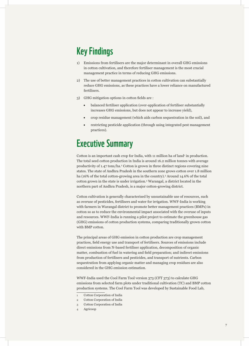
Key Findings1) Emissions from fertilisers are the major determinant in overall GHG emissions

in cotton cultivation, and therefore fertiliser management is the most crucial management practice in terms of reducing GHG emissions.

2) The use of better management practices in cotton cultivation can substantially reduce GHG emissions, as these practices have a lower reliance on manufactured fertilisers.

3) GHG mitigation options in cotton fi elds are :

balanced fertiliser application (over-application of fertiliser substantially increases GHG emissions, but does not appear to increase yield),

crop residue management (which aids carbon sequestration in the soil), and

restricting pesticide application (through using integrated pest management practices).

Executive SummaryCotton is an important cash crop for India, with 11 million ha of land1 in production. The total seed cotton production in India is around 16.2 million tonnes with average productivity of 1.47 tons/ha.2 Cotton is grown in three distinct regions covering nine states. The state of Andhra Pradesh in the southern zone grows cotton over 1.8 million ha (16% of the total cotton-growing area in the country).3 Around 14.6% of the total cotton grown in the state is under irrigation.4 Warangal, a district located in the northern part of Andhra Pradesh, is a major cotton-growing district.

Cotton cultivation is generally characterised by unsustainable use of resources, such as overuse of pesticides, fertilisers and water for irrigation. WWF-India is working with farmers in Warangal district to promote better management practices (BMPs) in cotton so as to reduce the environmental impact associated with the overuse of inputs and resources. WWF-India is running a pilot project to estimate the greenhouse gas (GHG) emissions of cotton production systems, comparing traditionally grown cotton with BMP cotton.

The principal areas of GHG emission in cotton production are crop management practices, fi eld energy use and transport of fertilisers. Sources of emissions include direct emissions from N-based fertiliser application, decomposition of organic matter, combustion of fuel in watering and fi eld preparation; and indirect emissions from production of fertilisers and pesticides, and transport of nutrients. Carbon sequestration from applying organic matter and managing crop residues are also considered in the GHG emission estimation.

WWF-India used the Cool Farm Tool version 373 (CFT 373) to calculate GHG emissions from selected farm plots under traditional cultivation (TC) and BMP cotton production systems. The Cool Farm Tool was developed by Sustainable Food Lab,

1 Cotton Corporation of India2 Cotton Corporation of India3 Cotton Corporation of India4 Agricoop

7

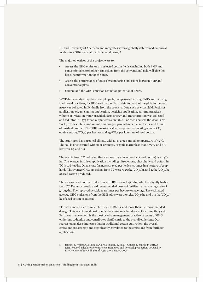
US and University of Aberdeen and integrates several globally determined empirical models in a GHG calculator (Hillier et al, 2011).5

The major objectives of the project were to:

Assess the GHG emissions in selected cotton fi elds (including both BMP and conventional cotton plots). Emissions from the conventional fi eld will give the baseline information for the area.

Assess the performance of BMPs by comparing emissions between BMP and conventional plots.

Understand the GHG emission reduction potential of BMPs.

WWF-India analysed 48 farm sample plots, comprising 27 using BMPs and 21 using traditional practices, for GHG estimation. Farm data for each of the plots in the year 2010 was collected individually from the growers. Data such as crop yield, fertiliser application, organic matter application, pesticide application, cultural practices, volume of irrigation water provided, farm energy and transportation was collected and fed into CFT 373 for an output emission table. For each analysis the Cool Farm Tool provides total emission information per production area, unit area and tonne of fi nished product. The GHG emission value is represented in kilograms of CO2 equivalent (kg/CO2e) per hectare and kg/CO2e per kilogram of seed cotton.

The study area has a tropical climate with an average annual temperature of 32°C. The soil is fi ne textured with poor drainage, organic matter less than 1.72%, and pH between 7.3 and 8.5.

The results from TC indicated that average fresh farm product (seed cotton) is 2.25T/ha. The average fertiliser application including nitrogenous, phosphatic and potash in TC is 1067kg/ha. On average farmers sprayed pesticides 35 times in a hectare of crop land. The average GHG emissions from TC were 3,236kg/CO2e/ha and 1.5kg/CO2e/kg of seed cotton produced.

The average seed cotton production with BMPs was 2.41T/ha, which is slightly higher than TC. Farmers mostly used recommended doses of fertiliser, at an average rate of 531kg/ha. They sprayed pesticides 12 times per hectare on average. The estimated average GHG emissions from the BMP plots were 1,032kg/CO2e/ha and 0.43kg/CO2e/kg of seed cotton produced.

TC uses almost twice as much fertiliser as BMPs, and more than the recommended dosage. This results in almost double the emissions, but does not increase the yield. Fertiliser management is the most crucial management practice in terms of GHG emissions reduction and contributes signifi cantly to the overall emissions. Our regression analysis indicates that in traditional cotton cultivation, the overall emissions are strongly and signifi cantly correlated to the emissions from fertiliser application.

5 Hillier, J, Walter, C, Malin, D, Garcia-Suarez, T, Mila-i-Canals, L, Smith, P. 2011. A farm-focused calculator for emissions from crop and livestock production, Journal of Environmental Modelling and Software, 26:1070-1078

8 | Cutting cotton carbon emissions - Finding from Warangal, India

1.0 IntroductionHuman activities, including burning fossil fuels such as coal and oil, and deforestation, have resulted in increasing concentrations of GHGs in the atmosphere. The GHG absorbs part of the energy being radiated from the surface of the Earth and traps it in the atmosphere, essentially acting like a blanket that makes the Earth’s surface warmer than it would be otherwise. These gases are considered as one of the principal sources of global warming. The major greenhouse gases include carbon dioxide (CO2), methane (CH4), nitrous oxide (N2O), fl uorocarbons and sulphur hexafl ouride (SF6).

The industrial sector is a major direct and indirect source of GHG emissions and therefore can play a potential role in mitigating emissions. In recent year, businesses have been making increased efforts to understand and address GHG emissions. Responsible businesses are paying greater attention to their carbon footprint: estimating GHG emissions throughout their company’s value chain – from production to disposal –is the fi rst step towards mitigating their impact. Focusing on GHG can generate consumer interest in the company and also set an example for other companies to follow. In the last few years, a range of organisations and governmental agencies across globe have published protocols and sectoral guidance for quantifying GHG emissions associated with voluntary reporting initiatives, such as the Carbon Disclosure Project (CDP)6 and Global Reporting Initiative (GRI)7. Many global industries are participating in consultations on mandatory GHG reporting regulations.

Carbon footprint is a hotspot issue in the textile industry, which is a signifi cant GHG emitter due to the size of its activity. From raw material production to retail of fi nished goods and further use by consumers, many processes and products consume signifi cant quantities of fossil fuel: from making fi bres, textiles and apparel products, to running stores, warehousing and logistics, to customers laundering their clothes. Apparel and textiles account for approximately 10% of the total carbon emissions.8 In country like the US, textiles are the fi fth largest contributor to CO2 emissions.9 The global textile and apparel industry is expected to grow from US$700 billion in 2011 to US$800 billion in 2015,10and a corresponding growth in associated emissions can be expected.

Global retailers run a number of initiatives to address their GHG emissions. Fashion retailer H&M in its 2011 sustainability report reported reduction of carbon emissions by 5% in one year. Several brands and retailers including Adidas, Levi’s, Puma, M&S,

6 “The Carbon Disclosure Project (CDP) is an independent not-for-profi t organization working to drive greenhouse gas emissions reduction by business. CDP provide a transformative global system for thousands of companies to measure, disclose, manage and share environmental information. When provided with the necessary information, market forces can be a major cause of change. CDP is working with the world’s largest investors, businesses and governments.” From www.cdproject.net [Accessed 8 February 13]

7 'The Global Reporting Initiative (GRI) is a non-profi t organization that promotes economic, environmental and social sustainability. GRI provides all companies and organizations with a comprehensive sustainability reporting framework that is widely used around the world.' From www.globalreporting.org [Accessed 8 February 13]

8 Zaffalon, V. 2010.Climate Change, Carbon Mitigation and Textiles, Textile World [online]. Available at: www.textileworld.com/Articles/2010/July/July_August_issue/Features/Climate_Change_Carbon_Mitigation_In_Textiles.html [Accessed 8 February 13]

9 Stone, B.2010. Carbon footprint and the Textile Industries. Bright Hub

10 AEPC Vision 2015

9

IKEA, Walmart and Tesco have undertaken supply chain initiatives for monitoring and reducing GHG emissions at factories.11 The majority of the assessments of GHG emissions are either centred around the full life cycle of garments, where emissions from raw material (cotton) production are a part of the assessment, or around a certain section within the supply chain. The present report attempts to assess the GHG emissions solely from cotton cultivation in a selected region of India on a pilot scale.

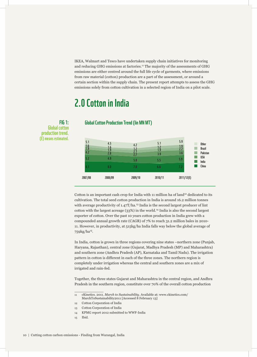
2.0 Cotton in India

Cotton is an important cash crop for India with 11 million ha of land12 dedicated to its cultivation. The total seed cotton production in India is around 16.2 million tonnes with average productivity of 1.47T/ha.13 India is the second largest producer of lint cotton with the largest acreage (33%) in the world.14 India is also the second largest exporter of cotton. Over the past 10 years cotton production in India grew with a compounded annual growth rate (CAGR) of 7% to reach 31.2 million bales in 2010-11. However, in productivity, at 515kg/ha India falls way below the global average of 759kg/ha15.

In India, cotton is grown in three regions covering nine states –northern zone (Punjab, Haryana, Rajasthan), central zone (Gujarat, Madhya Pradesh (MP) and Maharashtra) and southern zone (Andhra Pradesh (AP), Karnataka and Tamil Nadu). The irrigation pattern in cotton is different in each of the three zones. The northern region is completely under irrigation whereas the central and southern zones are a mix of irrigated and rain-fed.

Together, the three states Gujarat and Maharashtra in the central region, and Andhra Pradesh in the southern region, constitute over 70% of the overall cotton production

11 cKinetics. 2011. March to Sustainability. Available at: www.ckinetics.com/MarchToSustainability2011 [Accessed 8 February 13]

12 Cotton Corporation of India13 Cotton Corporation of India14 KPMG report 2012 submitted to WWF-India15 Ibid.

2007/08 2008/09 2009/10 2010/11 2011/12(E)

8.1 8.0 7.0 6.6 7.2

5.2 4.95.0 5.5 5.9

4.2 2.8 2.7 3.9 3.6

1.9 1.9 2.11.9 2.2

1.6 1.6 1.21.2 1.9

5.1 4.5 4.25.1

5.9

China

India

USA

Pakistan

Brazil

Other

Global Cotton Production Trend (Iin MN MT)FIG 1: Global cotton

production trend. (E) means estimated.


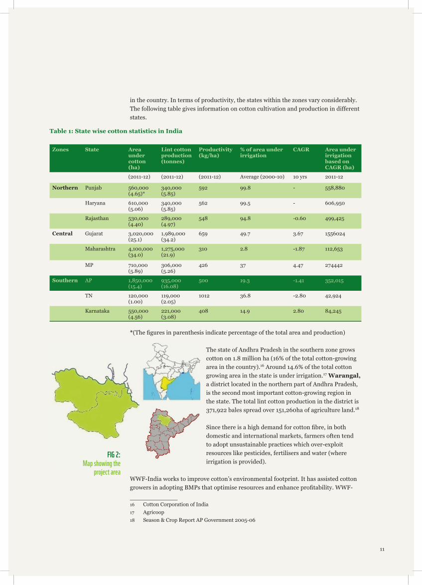
in the country. In terms of productivity, the states within the zones vary considerably. The following table gives information on cotton cultivation and production in different states.

*(The fi gures in parenthesis indicate percentage of the total area and production)

The state of Andhra Pradesh in the southern zone grows cotton on 1.8 million ha (16% of the total cotton-growing area in the country).16 Around 14.6% of the total cotton growing area in the state is under irrigation.17 Warangal, a district located in the northern part of Andhra Pradesh, is the second most important cotton-growing region in the state. The total lint cotton production in the district is 371,922 bales spread over 151,260ha of agriculture land.18

Since there is a high demand for cotton fi bre, in both domestic and international markets, farmers often tend to adopt unsustainable practices which over-exploit resources like pesticides, fertilisers and water (where irrigation is provided).

WWF-India works to improve cotton’s environmental footprint. It has assisted cotton growers in adopting BMPs that optimise resources and enhance profi tability. WWF-

16 Cotton Corporation of India17 Agricoop18 Season & Crop Report AP Government 2005-06

Table 1: State wise cotton statistics in India

Zones State Area under cotton (ha)

Lint cotton production (tonnes)

Productivity (kg/ha)

% of area under irrigation

CAGR Area under irrigation based on CAGR (ha)

(2011-12) (2011-12) (2011-12) Average (2000-10) 10 yrs 2011-12

Northern Punjab 560,000(4.65)*

340,000(5.85)

592 99.8 - 558,880

Haryana 610,000(5.06)

340,000(5.85)

562 99.5 - 606,950

Rajasthan 530,000(4.40)

289,000(4.97)

548 94.8 -0.60 499,425

Central Gujarat 3,020,000(25.1)

1,989,000(34.2)

659 49.7 3.67 1556024

Maharashtra 4,100,000(34.0)

1,275,000(21.9)

310 2.8 -1.87 112,653

MP 710,000(5.89)

306,000(5.26)

426 37 4.47 274442

Southern AP 1,850,000(15.4)

935,000(16.08)

500 19.3 -1.41 352,015

TN 120,000(1.00)

119,000(2.05)

1012 36.8 -2.80 42,924

Karnataka 550,000(4.56)

221,000(3.08)

408 14.9 2.80 84,245

FIG 2: Map showing the

project area

11

India has helped to infl uence the cotton farmers in India towards implementing BMPs, in order to mainstream environmentally sustainable agricultural practices. The success of the project is evident as several farmers in different cotton-growing states are participating to produce cotton through BMPs. The results have been impressive, greatly reducing inputs while maintaining or improving productivity. However, BMPs have not been examined either in terms of GHG emissions or the impact of chemicals on water quality. The project Greenhouse-gas emissions from cotton farms in Warangal district of Andhra Pradesh made an attempt to understand these issues and develop a blueprint to address them.

This pilot study undertaken by WWF-India has attempted to estimate the GHG emissions in cotton production systems in two types of cotton fi elds –involving traditional practices and BMPs. The principal areas of GHG emissions in cotton production are crop management practices, fi eld energy use and transport of fertilisers. The direct GHG emissions originate from N-based fertiliser application, decomposition of organic matter and combustion of fuel in watering and fi eld preparation; indirect emissions arise from the production of fertilisers and pesticides and transport of nutrients. Carbon sequestration from organic matter application and crop residue management is also considered in estimating the net emissions.

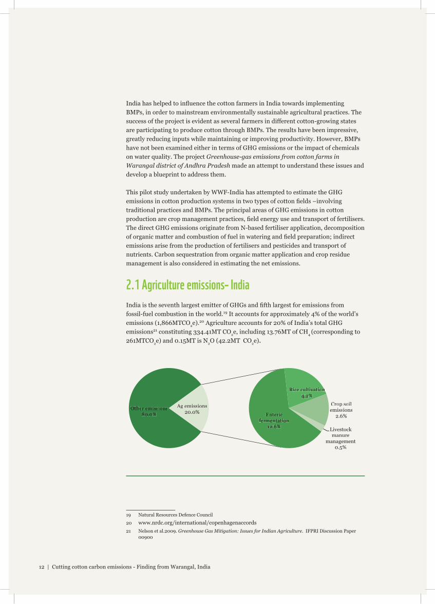
2.1 Agriculture emissions– India

India is the seventh largest emitter of GHGs and fi fth largest for emissions from fossil-fuel combustion in the world.19 It accounts for approximately 4% of the world’s emissions (1,866MTCO2e).20 Agriculture accounts for 20% of India’s total GHG emissions21 constituting 334.41MT CO2e, including 13.76MT of CH4 (corresponding to 261MTCO2e) and 0.15MT is N2O (42.2MT CO2e).

19 Natural Resources Defence Council

20 www.nrdc.org/international/copenhagenaccords21 Nelson et al.2009. Greenhouse Gas Mitigation: Issues for Indian Agriculture. IFPRI Discussion Paper

00900

Crop soilemissions

2.6%

Livestock manure

management0.5%

Other emissions80.0% Enteric

feff rmentation12.6%

RiRR ce cultivationn4.2%

m

AgA emissions20.0%


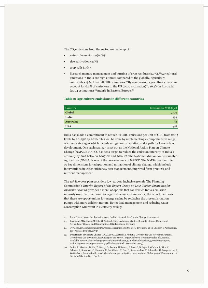
The CO2 emissions from the sector are made up of:

• enteric fermentation(63%)

• rice cultivation (21%)

• crop soils (13%)

• livestock manure management and burning of crop residues (2.7%).22Agricultural emissions in India are high at 20%: compared to the globally, agriculture contributes 13% of overall GHG emissions.23By comparison, agriculture emissions account for 6.3% of emissions in the US (2010 estimation)24, 16.3% in Australia (2004 estimation) 25and 3% in Eastern Europe.26

Table 2: Agriculture emissions in different countries

Country Emissions(MTCO2e)

Global 5,729

India 334

Australia 93

USA 428

India has made a commitment to reduce its GHG emissions per unit of GDP from 2005 levels by 20-25% by 2020. This will be done by implementing a comprehensive range of climate strategies which include mitigation, adaptation and a path for low-carbon development. One such strategy is set out as the National Action Plan on Climate Change (NAPCC). NAPCC has set a target to reduce the emission intensity of India’s economy by 20% between 2007-08 and 2016-17. The National Mission for Sustainable Agriculture (NMSA) is one of the core elements of NAPCC. The NMSA has identifi ed 10 key dimensions for adaptation and mitigation of climate change, which include interventions in water effi ciency, pest management, improved farm practices and nutrient management.

The 12th fi ve-year plan considers low-carbon, inclusive growth. The Planning Commission’s Interim Report of the Expert Group on Low Carbon Strategies for Inclusive Growth provides a menu of options that can reduce India’s emission intensity over the timeframe. As regards the agriculture sector, the report mentions that there are opportunities for energy saving by replacing the present irrigation pumps with more effi cient motors. Better load management and reducing water consumption will result in electricity savings.

22 India Green House Gas Emission 2007: Indian Network for Climate Change Assessment

23 Rosegrant,MW,Ewing,M,Yohe,G,Burton,I,Huq,S,Valmonte-Santos, R. 2008. Climate Change and Agriculture: Threats and Opportunities.GTZ.Eschborn, Germany

24 www.epa.gov/climatechange/Downloads/ghgemissions/US-GHG-Inventory-2012-Chapter-6-Agriculture.pdf [Accessed 8 February 13]

25 Department of Climate Change (DCC).2009. Australia’s National Greenhouse Gas Accounts: National Greenhouse Gas Inventory Accounting for the Kyoto Target.Canberra: Commonwealth of Australia. Available at www.climatechange.gov.au/climate-change/y/media/publications/greenhouse-report/national-greenhouse-gas-inventory-pdf.ashx (verifi ed 1 December 2009).

26 Smith, P, Martino, D, Cai, Z, Gwary, D, Janzen, H,Kumar, P, Mccarl, B, Ogle, S, O’Mara, F, Rice, C, Scholes, R, Sirotenko, O, Howden, M, McAllister, T, Pan, G, Romanenkov, V, Schneider, U, Towprayoon, S, Wattenbach, MandJSmith. 2008. Greenhouse gas mitigation in agriculture. Philosophical Transactions of the Royal Society B 27: 89–813

13

2.2 Emissions from cotton production

This section attempts to understand the emissions from cotton production by reviewing global and national studies. Though a few global studies pertaining to GHG emissions in cotton production were found, no such study at the national level has been conducted specifi cally for cotton. In India, methane and nitrous oxide emissions have been estimated for irrigated crops like rice and wheat, leguminous crops and livestock. It is evident that most of the concerns around GHG emissions in agriculture are directed towards irrigated crops with high input usage as mentioned above. Cotton is generally considered an environmentally challenging crop because of its high pesticide use, further raising the issue of contaminants in water and soil. The area under crops like rice and wheat has shown stagnancy (rice acreage decreased at a CAGR of -0.49% from 2000-01 to 2010-1127; wheat acreage increased by only 0.51% from 1993-94 to 2004-0528) whereas the area under cotton cultivation has been increasing at a CAGR of 3% over the last 12 years.29 The increase in area is associated with an increase in inputs, both chemicals and irrigation, suggesting cotton is making up an increasing proportion of agricultural inputs. This makes understanding emissions from cotton production increasingly important.

Since cotton forms an important raw material for apparel and textile industries, most studies focus on cotton production as part of the overall emissions estimate in the supply chain. Reducing emissions from cotton production is clearly an important part of many businesses’ corporate sustainability strategies.

In the entire supply chain of garment/textiles (excluding the consumer-use part – washing and drying), the fi bre production phase emits the most GHGs30. Cotton Incorporated (2009) estimated that the GHG emissions were around 1.8kgCO2e/kg of fi bre. This estimate was based on averaging data from three studies conducted by Nelson et al (2009), Matlock et al (2008 & 2009) and Keystone (2009). In a similar study of Australian cotton, the GHG emissions from cotton production were estimated at 2.5 kg CO2e/kg of fi bre (Pyke, 2009)31; this included emissions from application of inputs (fertilisers, chemicals, fuel and electricity). Grace32 estimated a net emission of 970kg CO2e/ha from mixed cotton farming in Australia. This estimation, however, included methane emissions from livestock. Marseni et al (2010)33 estimated GHG emissions in three cotton farming systems (two in different spacing’s of dry-land farming systems and the other in an irrigated system) in the Darling Downs region, Queensland, Australia. This estimate considered emissions from production, packaging and storage; transportation of farm inputs (fertilisers, agrochemicals, farm machinery); extraction, production and use of electricity for irrigation; and of N2O from soils due to N-fertiliser application. The study estimated that the highest

27 Project Wilderness, KPMG report submitted to WWF-India.2012

28 Handbook on India Statistics 2005-06, Reserve Bank of India

29 Project Wilderness, KPMG Report submitted to WWF-India. 2012

30 Steinberger, Friot, Jolliet & Erkman. 2009 “A Spatially-explicit Life Cycle Inventory of the Global Textile Chain,” The International Journal of Life Cycle Assessment, Springer Berlin/Heidelberg, May 2009

31 Pyke, B. 2009. The Impacts of Carbon Trading on the Cotton Industry. 68thICAC Plenary, Fourth Breakout Session, Thursday 10 September, 2009. Cape Town. Available at:www.icac.org/meetings/plenary/68_cape_town/documents/bo4/bo4_e_pyke.pdf [Accessed 8 February 13]

32 Grace, P. A cotton farm’s carbon and greenhouse footprint

33 Maraseni, TN, Cockfi eld, G and J Maroulis. 2010. Journal of Agricultural Science 148: 501–510


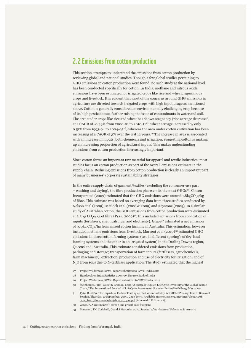
quantities of GHGs are emitted from irrigated cotton farming (4,841kg CO2e/ha), followed by dry-land solid-plant (1,367kg CO2e/ha) and dry-land double-skip (1,274kg CO2e/ha).

It is evident from the above that it is impossible to give a single defi nitive fi gure for emissions from cotton production. The emission values vary greatly because the studies were undertaken in different regions, and the scope and methods of the assessments were different.

Table 3: Summary of analysis of various studies conducted to estimate GHG emissions of cotton cultivation

Study Location Value Unit Scope of the assessment

Cotton Incorporated (2009)

United States 1.8 kg CO2e/kg of fi bre

Not clear – takes average of three estimates from three authors

Australian Cotton Life Cycle Assessment (2009)

Australia 2.5 kg CO2e/kg of fi bre

Emissions from input application – fertilisers, chemicals, fuel and electricity

Grace, P. Australia 970 kg CO2e/ha Residue emissions, nitrogenous fertiliser emissions, carbon stock exchange, livestock emissions, energy emissions

Marseni (2010)

Australia 4,841 (irrigated)1,367 (dry-land)1,274 (dry-land, skip method)

KgCO2e/ha Emissions from production, packaging, storage and transportation of farm inputs (fertilisers, agrochemicals, farm machinery);extraction, production and use of electricity for irrigation;N2O from soils due to N-fertiliser application

Most of the work on estimating GHG emissions in cotton cultivation is part of the overall textile life cycle analysis. Understanding the emissions from each component of the textile supply chain is essential for reducing carbon emissions and improving sustainability. Emissions from the production side of raw materials refl ect the pattern of resource use and environmental sustainability in the agriculture production system in question.

15

3.0 The project: Greenhouse-gas emissions from cotton farms in Warangal district of Andhra PradeshThe project Greenhouse-gas emissions from cotton farms in Warangal district of Andhra Pradesh was conducted by WWF-India with support from Marks & Spencer through WWF-UK in 2010-11. This was a pilot project conducted in two blocks of Warangal district, Andhra Pradesh.

3.1 Participating partners in the project

Marks & Spencer (M&S) is one of the UK’s leading retailers with a customer base of around 21 million visiting the retail stores every week.34 The company is committed to sustainability in its businesses and supply chain. M&S is one of the fi rst global retailers to have carbon-neutral operations. Its Plan A programme sets out 180 commitments to achieve by 2015 with the ultimate goal of becoming the world’s most sustainable retailer. Through Plan A, M&S is working with customers and suppliers to combat climate change, reduce waste, use sustainable raw materials, trade ethically and help customers to lead healthier lives.35 To reinforce its long-term environmental objectives on clothing and textiles, M&S has supported WWF in helping reduce the overall environmental impact of the cotton that it sources from India through the Better Cotton Initiative.

WWF-UK is committed to protect the planet and its diversity – people, animals and habitats. It helps businesses manage their environmental footprint while building sustainability into their brand, their customer and investor communications, and their engagement with government. WWF-UK sees a One Planet Future, in which business makes a restorative contribution to the natural world, supports Earth’s adaptation to a changing climate and benefi ts human well-being. This in turn will help to build businesses that last. WWF-UK guides companies towards greater effi ciencies in natural resource use and best practices in carbon management, and helps them respond to growing consumer demand for environmentally sound products and services – all of which enhance business competitiveness.

WWF-UK is helping M&S to achieve Plan A. M&S is working with WWF on environmental projects in its supply chain as it looks to substantially increase its sourcing of sustainable raw materials, with a particular focus on agriculture, marine and freshwater.

WWF-India is the implementing partner. Cotton is an important crop in India, but has a major environmental impact with serious repercussion on water quality and quantity. WWF-India works in different agro-climatic regions, running locally adapted projects that take into account the environmental benefi ts; income and education

34 Marks & Spencer.2011.How do we business report. Available at: plana.marksandspencer.com/media/pdf/how_we-do_business_report_2011.pdf [Accessed 8 February 13]

35 www.plana.marksandspencer.com/about


levels of farmers and other stakeholders; environmental policies; and industry support for BMPs.

WWF-India runs various interventions to achieve sustainability in cotton production, from environmental stability in the crop production process to market transformation initiatives:

Assessment: WWF-India’s Sustainable Cotton project is taking stock of the ecological footprint and assessing the hydrological risks associated with cotton production. This will help create a roadmap for long-term environmental sustainability for cotton.

Application: The Sustainable Cotton project is working towards developing improved sustainable cotton production systems. Farmers, by adopting BMPs, are equipped to produce quality cotton using environment-friendly organic fertilisers produced from locally available resources. The project uses an integrated approach by developing water, nutrient, pest and disease management practices for cotton production systems. It has created a ripple effect among farmers in the Warangal district of Andhra Pradesh, as well as Jalna and Aurangabad districts of Maharashtra.

Market engagement: WWF’s overall strategy for cotton is to move the mainstream commodity market towards sustainable production, both by increasing the demand for sustainable cotton from globally signifi cant retailers and brands and by supporting farmers to move towards more sustainable and more economical cotton production methods. The aim of this strategy is to reduce the ecological footprint in the entire cotton chain, from production to retail, ultimately demonstrating positive impacts on key ecosystems and river basins.36 WWF-India is a part of the global Better Cotton Initiative (BCI). WWF-India has given momentum to the BCI in India. WWF is also working with global retailers to facilitate implementation of the BCI.

The project fi ts into WWF’s overall goal to develop an equitable low-carbon economy and work on low-carbon development. It also contributes to WWF’s Market Transform Initiative (MTI), for which cotton is a priority commodity, by assessing GHGs and improving understanding of the potential role of BMPs in a low-carbon cotton production system.

36 WWF-India. 2012. Cotton sustainability: Business and Environment Approach

17

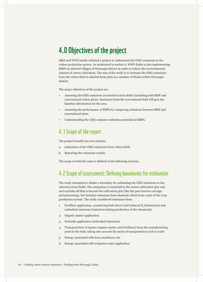
4.0 Objectives of the projectM&S and WWF jointly initiated a project to understand the GHG emissions in the cotton production system. As mentioned in section 2, WWF-India is also implementing BMPs in selected villages of Warangal district in order to reduce the environmental impacts of cotton cultivation. The aim of the study is to estimate the GHG emissions from the cotton fi eld in selected farm plots in a number of blocks within Warangal district.

The major objectives of the project are:

• Assessing the GHG emissions in selected cotton fi elds (including both BMP and conventional cotton plots). Emissions from the conventional fi eld will give the baseline information for the area.

• Assessing the performance of BMPs by comparing emissions between BMP and conventional plots.

• Understanding the GHG emission reduction potential of BMPs.

4.1 Scope of the report

The project broadly has two sections:

a. estimation of the GHG emissions from cotton fi elds

b. Reporting the emissions results.

The scope in both the cases is defi ned in the following sections:

4.2 Scope of assessment: Defi ning boundaries for estimation

The study attempted to defi ne a boundary for estimating the GHG emissions in the selected cotton fi elds. The estimation is restricted to the cotton cultivation plot only and excludes all that is beyond the cultivation plot (like the post-harvest carriage and processing), but includes emissions from elements which form a part of the crop production system. The study considered emissions from:

1. Fertiliser application, considering both direct (soil-induced N2Oemissions) and embodied emissions (emissions during production of the chemicals)

2. Organic matter application

3. Pesticide application (embodied emissions)

4. Transportation of inputs (organic matter and fertilisers) from the manufacturing point to the fi eld, taking into account the mode of transportation (rail or road)

5. Energy associated with farm machinery use

6. Energy associated with irrigation water application


7. Soil carbon stock changes because of soil management and organic amendments, and sequestration through organic matter application.

The study did not consider the emissions from livestock, since these do not form a part of the estimation boundary: while most of the farmers in the pilot own cattle, which emit GHGs, they are kept away from the cotton fi eld. In some cases, the farmers may use a bullock-driven plough for land preparation; but since the emissions from this animal would have occurred whether it not it was used in the cotton fi eld, they are not included in the estimation.

Out of the six major GHGs, only three (CO2, N2O and CH4) are relevant to agriculture. The present study addresses only two CO2 and N2O. The principal sources of GHG emissions from cotton farming systems are:

• CO2 from urea application, combustion of fuel, energy consumption in the form of electricity etc., production of fertilisers, pesticides

• N2O during transformation of both mineral fertilisers and organic nitrogen applied to the soil.

All the emissions are expressed as kg/CO2e/ha or kg/CO2e/kg of seed cotton. Since livestock emissions are not considered, no methane emission is envisaged within the project boundaries. For N2O, we used a Global Warming Potential (GWP) factor of 296.

4.3 Scope of this report

This review focuses on GHG emissions, and does not explore non-GHG environmental or social issues in the cotton production sector. The report tries to understand the major contributing factors of GHG emissions and the potential of practices to reduce emissions in the study area. It does not attempt to draft a mitigation plan, which is beyond the scope of the study.

19

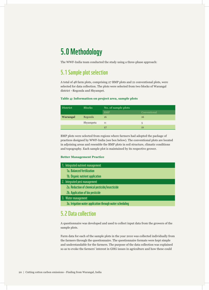
5.0 MethodologyThe WWF-India team conducted the study using a three-phase approach:

5.1 Sample plot selection

A total of 48 farm plots, comprising 27 BMP plots and 21 conventional plots, were selected for data collection. The plots were selected from two blocks of Warangal district –Regonda and Shyampet.

Table 4: Information on project area, sample plots

District Blocks No. of sample plots

BMP Conventional

Warangal Regonda 16 16

Shyampeta 11 5

27 21

BMP plots were selected from regions where farmers had adopted the package of practices designed by WWF-India (see box below). The conventional plots are located in adjoining areas and resemble the BMP plots in soil structure, climatic conditions and topography. Each sample plot is maintained by its respective grower.

Better Management Practice

5.2 Data collection

A questionnaire was developed and used to collect input data from the growers of the sample plots.

Farm data for each of the sample plots in the year 2010 was collected individually from the farmers through the questionnaire. The questionnaire formats were kept simple and understandable for the farmers. The purpose of the data collection was explained so as to evoke the farmers’ interest in GHG issues in agriculture and how these could

1. Integrated nutrient management

1a. Balanced fertilization

1b. Organic nutrient application

2. Integrated pest management

2a. Reduction of chemical pesticide/insecticide

2b. Application of bio pesticide

3. Water management

3a. Irrigation water application through water scheduling


affect them. The subject seems to be complex for small to medium land holders at this point. However, they could relate to climate/weather vagaries raising concerns in crop production. Data collected related to fertiliser application, fertiliser brand (to understand the manufacture), organic matter application, pesticide application, volume of irrigation water provided, farm energy requirement, distance inputs were transported by farmers and mode of transportation.

The fertiliser brand name meant we could identify the manufacturer, which helped in calculating the distance and mode of transport used from the factory to the retail outlet.

The farm energy data for irrigation was calculated on the basis of the power of the pump used in irrigation (represented in HP) and hours of pumping for respective farmers.

Publicly available secondary sources, mostly local, were scanned to collect information such as the C:N ratio of vermicompost, farmyard manure, seed cotton: fi bre ratio, and seed cotton: biomass ratio.

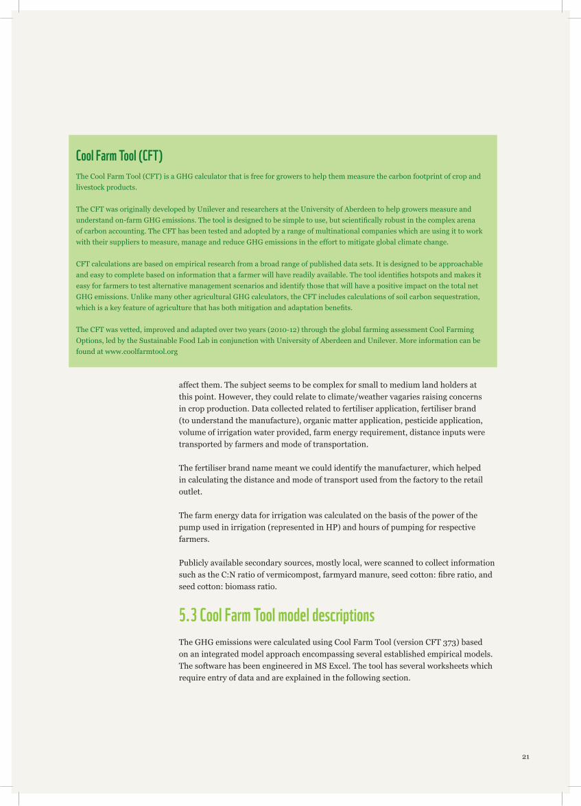
5.3 Cool Farm Tool model descriptions

The GHG emissions were calculated using Cool Farm Tool (version CFT 373) based on an integrated model approach encompassing several established empirical models. The software has been engineered in MS Excel. The tool has several worksheets which require entry of data and are explained in the following section.

The Cool Farm Tool (CFT) is a GHG calculator that is free for growers to help them measure the carbon footprint of crop and livestock products.

The CFT was originally developed by Unilever and researchers at the University of Aberdeen to help growers measure and understand on-farm GHG emissions. The tool is designed to be simple to use, but scientifi cally robust in the complex arena of carbon accounting. The CFT has been tested and adopted by a range of multinational companies which are using it to work with their suppliers to measure, manage and reduce GHG emissions in the effort to mitigate global climate change.

CFT calculations are based on empirical research from a broad range of published data sets. It is designed to be approachable and easy to complete based on information that a farmer will have readily available. The tool identifi es hotspots and makes it easy for farmers to test alternative management scenarios and identify those that will have a positive impact on the total net GHG emissions. Unlike many other agricultural GHG calculators, the CFT includes calculations of soil carbon sequestration, which is a key feature of agriculture that has both mitigation and adaptation benefi ts.

The CFT was vetted, improved and adapted over two years (2010-12) through the global farming assessment Cool Farming Options, led by the Sustainable Food Lab in conjunction with University of Aberdeen and Unilever. More information can be found at www.coolfarmtool.org

Cool Farm Tool (CFT)

21

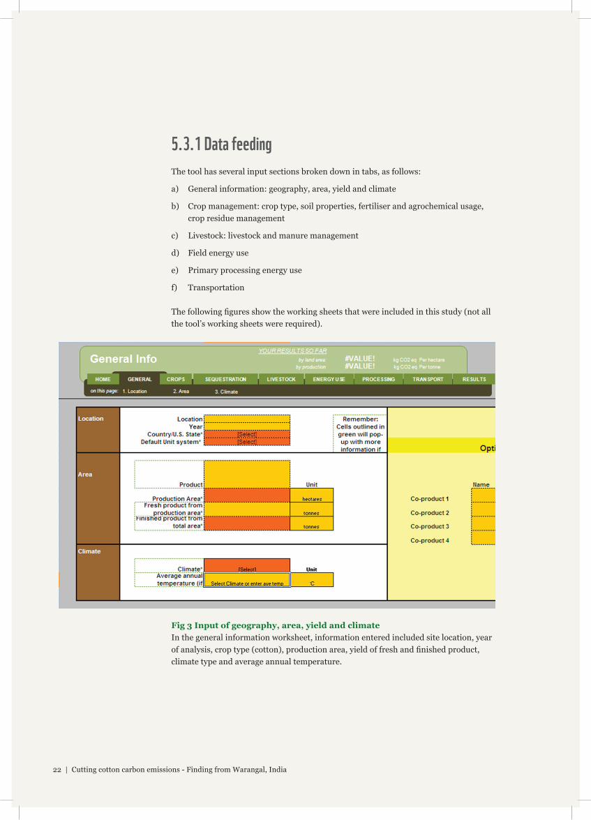
5.3.1 Data feeding

The tool has several input sections broken down in tabs, as follows:

a) General information: geography, area, yield and climate

b) Crop management: crop type, soil properties, fertiliser and agrochemical usage, crop residue management

c) Livestock: livestock and manure management

d) Field energy use

e) Primary processing energy use

f) Transportation

The following fi gures show the working sheets that were included in this study (not all the tool’s working sheets were required).

Fig 3 Input of geography, area, yield and climateIn the general information worksheet, information entered included site location, year of analysis, crop type (cotton), production area, yield of fresh and fi nished product, climate type and average annual temperature.


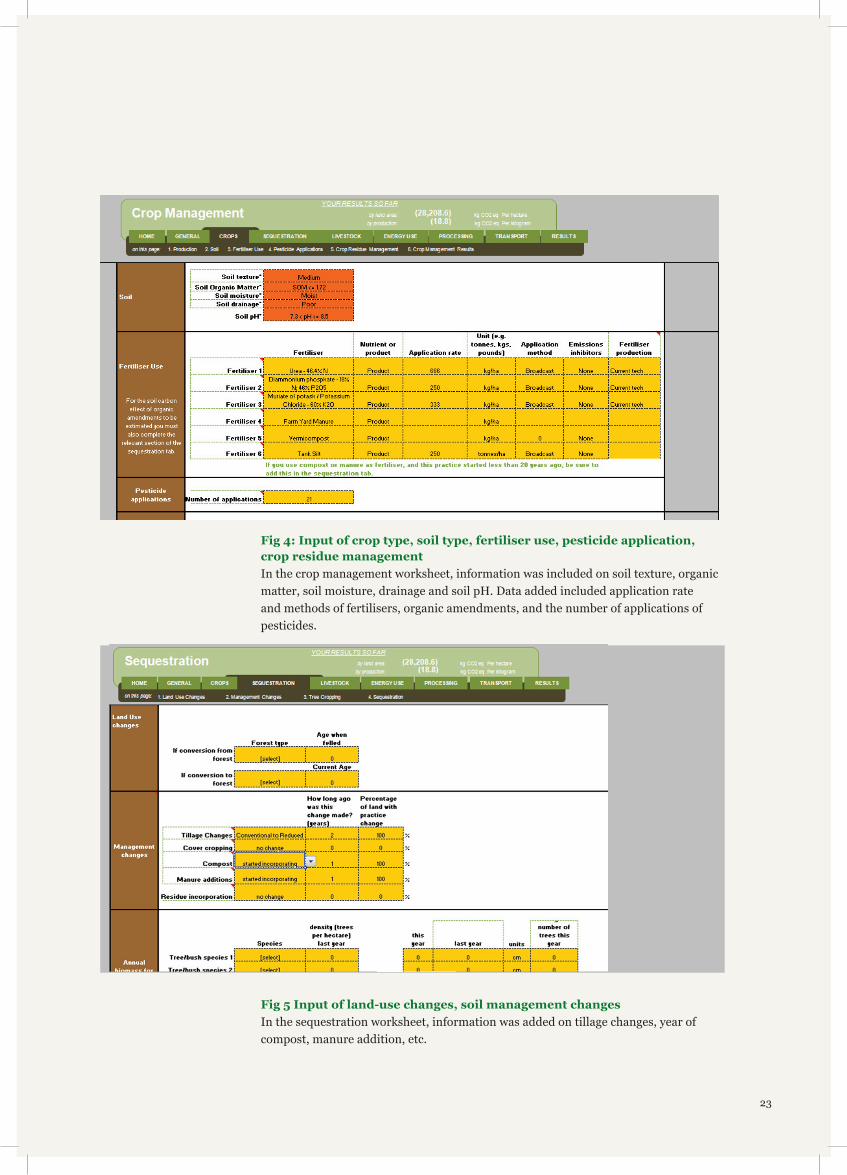
Fig 4: Input of crop type, soil type, fertiliser use, pesticide application, crop residue managementIn the crop management worksheet, information was included on soil texture, organic matter, soil moisture, drainage and soil pH. Data added included application rate and methods of fertilisers, organic amendments, and the number of applications of pesticides.

Fig 5 Input of land-use changes, soil management changesIn the sequestration worksheet, information was added on tillage changes, year of compost, manure addition, etc.

23

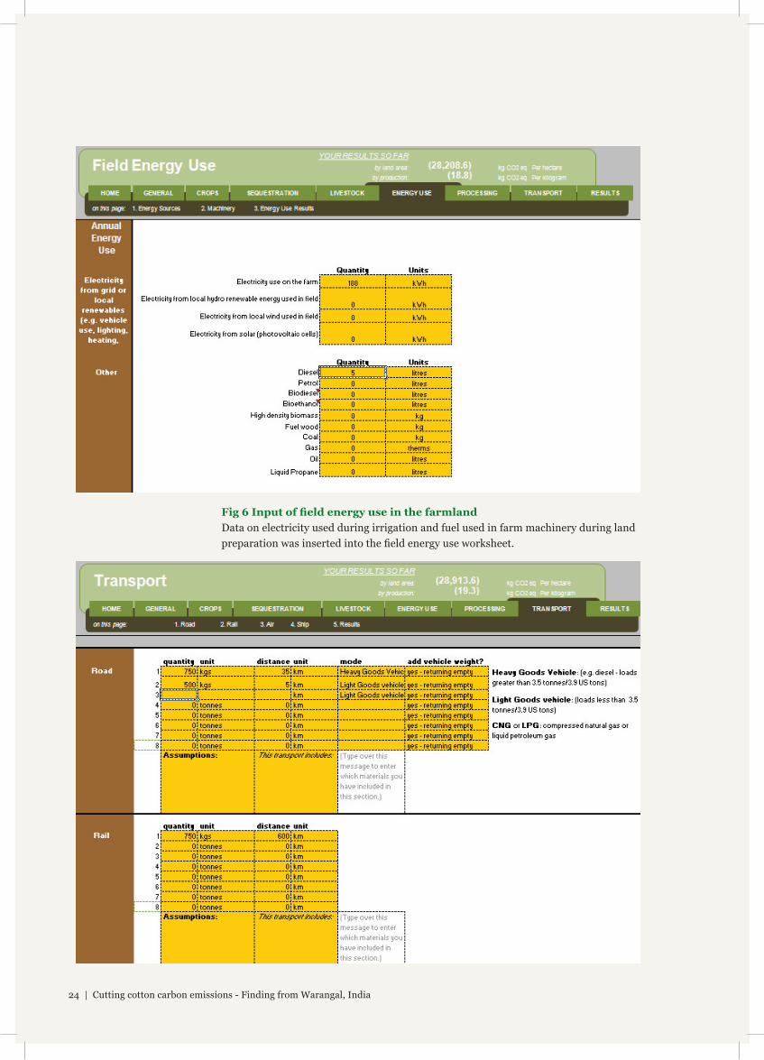
Fig 6 Input of fi eld energy use in the farmlandData on electricity used during irrigation and fuel used in farm machinery during land preparation was inserted into the fi eld energy use worksheet.


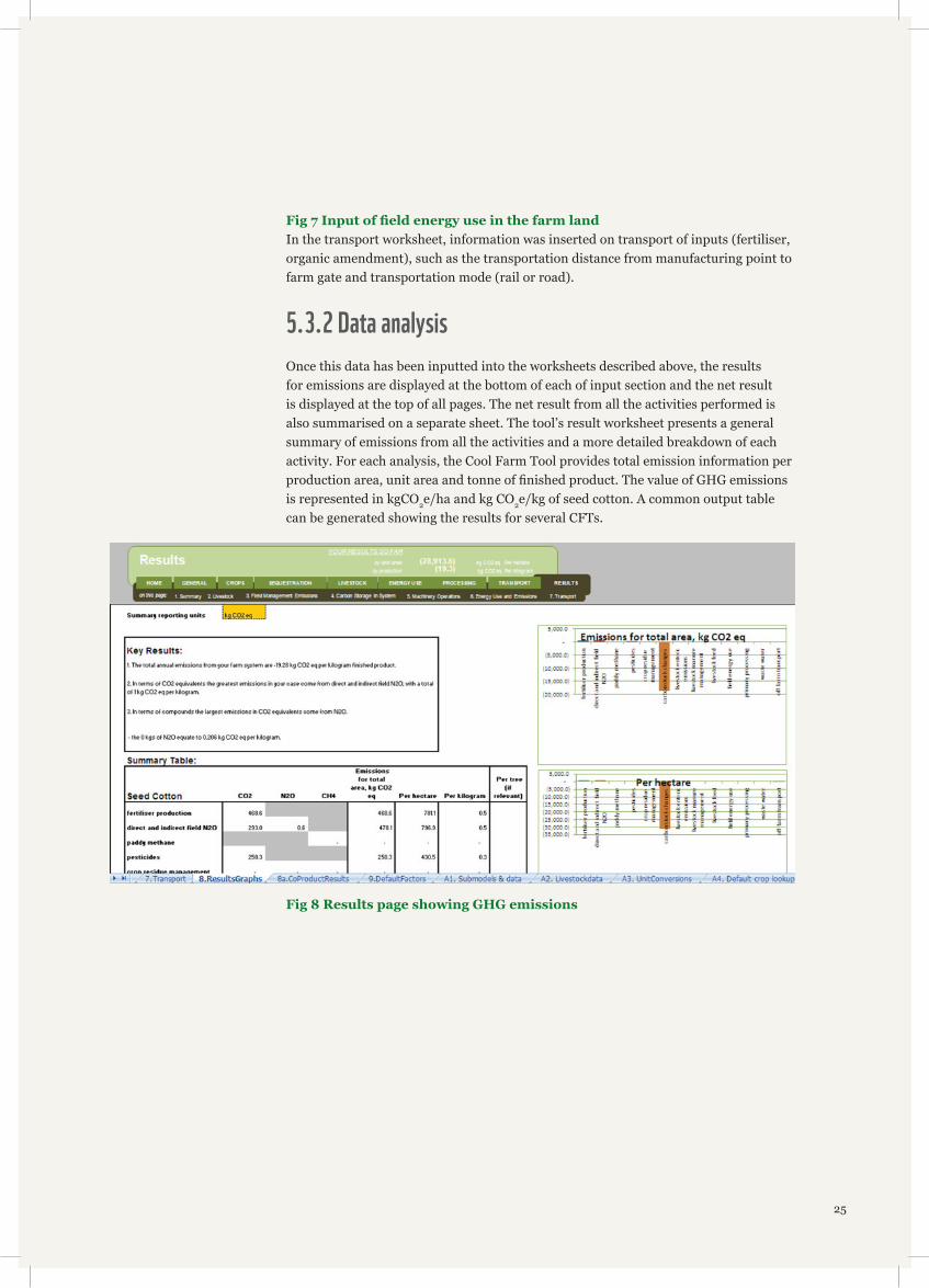
Fig 7 Input of fi eld energy use in the farm landIn the transport worksheet, information was inserted on transport of inputs (fertiliser, organic amendment), such as the transportation distance from manufacturing point to farm gate and transportation mode (rail or road).

5.3.2 Data analysis

Once this data has been inputted into the worksheets described above, the results for emissions are displayed at the bottom of each of input section and the net result is displayed at the top of all pages. The net result from all the activities performed is also summarised on a separate sheet. The tool’s result worksheet presents a general summary of emissions from all the activities and a more detailed breakdown of each activity. For each analysis, the Cool Farm Tool provides total emission information per production area, unit area and tonne of fi nished product. The value of GHG emissions is represented in kgCO2e/ha and kg CO2e/kg of seed cotton. A common output table can be generated showing the results for several CFTs.

Fig 8 Results page showing GHG emissions

25

6.0 Results and discussion6.1 General information

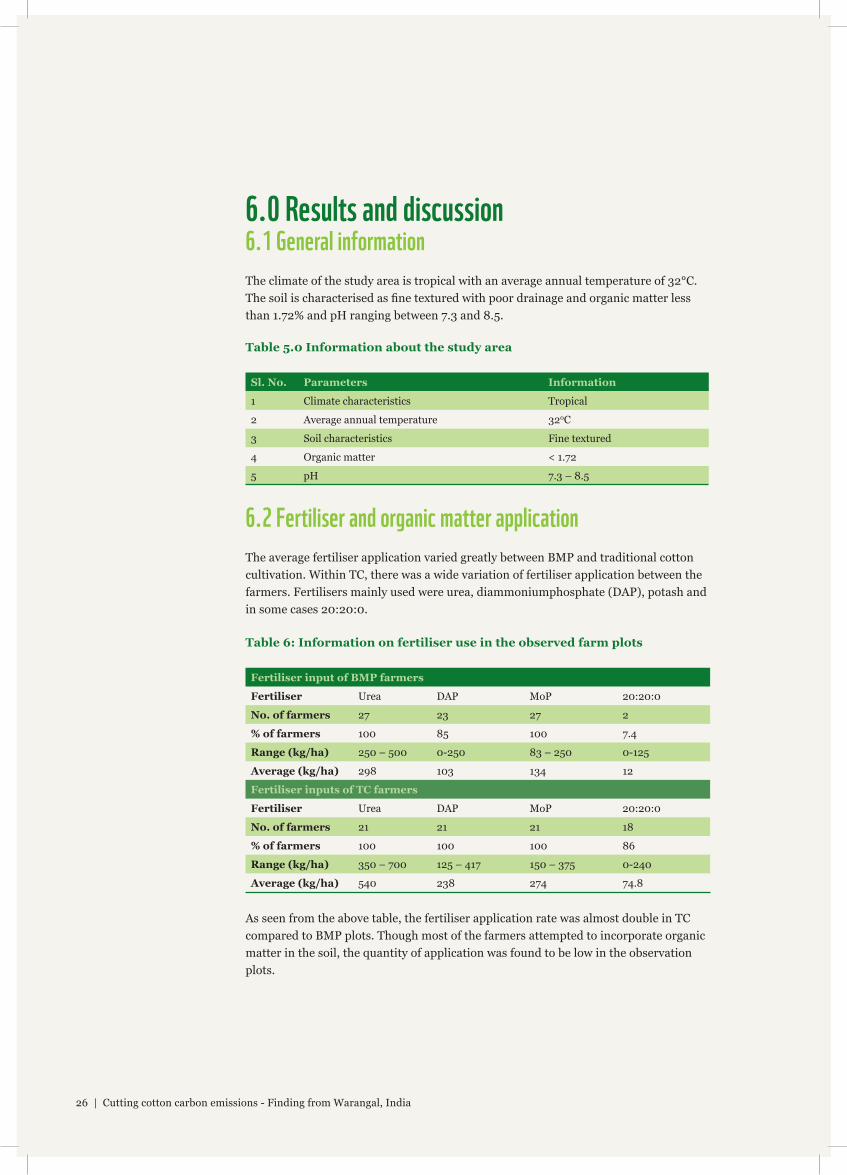
The climate of the study area is tropical with an average annual temperature of 32°C. The soil is characterised as fi ne textured with poor drainage and organic matter less than 1.72% and pH ranging between 7.3 and 8.5.

Table 5.0 Information about the study area

Sl. No. Parameters Information

1 Climate characteristics Tropical

2 Average annual temperature 320C

3 Soil characteristics Fine textured

4 Organic matter < 1.72

5 pH 7.3 – 8.5

6.2 Fertiliser and organic matter application

The average fertiliser application varied greatly between BMP and traditional cotton cultivation. Within TC, there was a wide variation of fertiliser application between the farmers. Fertilisers mainly used were urea, diammoniumphosphate (DAP), potash and in some cases 20:20:0.

Table 6: Information on fertiliser use in the observed farm plots

Fertiliser input of BMP farmers

Fertiliser Urea DAP MoP 20:20:0

No. of farmers 27 23 27 2

% of farmers 100 85 100 7.4

Range (kg/ha) 250 – 500 0-250 83 – 250 0-125

Average (kg/ha) 298 103 134 12

Fertiliser inputs of TC farmers

Fertiliser Urea DAP MoP 20:20:0

No. of farmers 21 21 21 18

% of farmers 100 100 100 86

Range (kg/ha) 350 – 700 125 – 417 150 – 375 0-240

Average (kg/ha) 540 238 274 74.8

As seen from the above table, the fertiliser application rate was almost double in TC compared to BMP plots. Though most of the farmers attempted to incorporate organic matter in the soil, the quantity of application was found to be low in the observation plots.


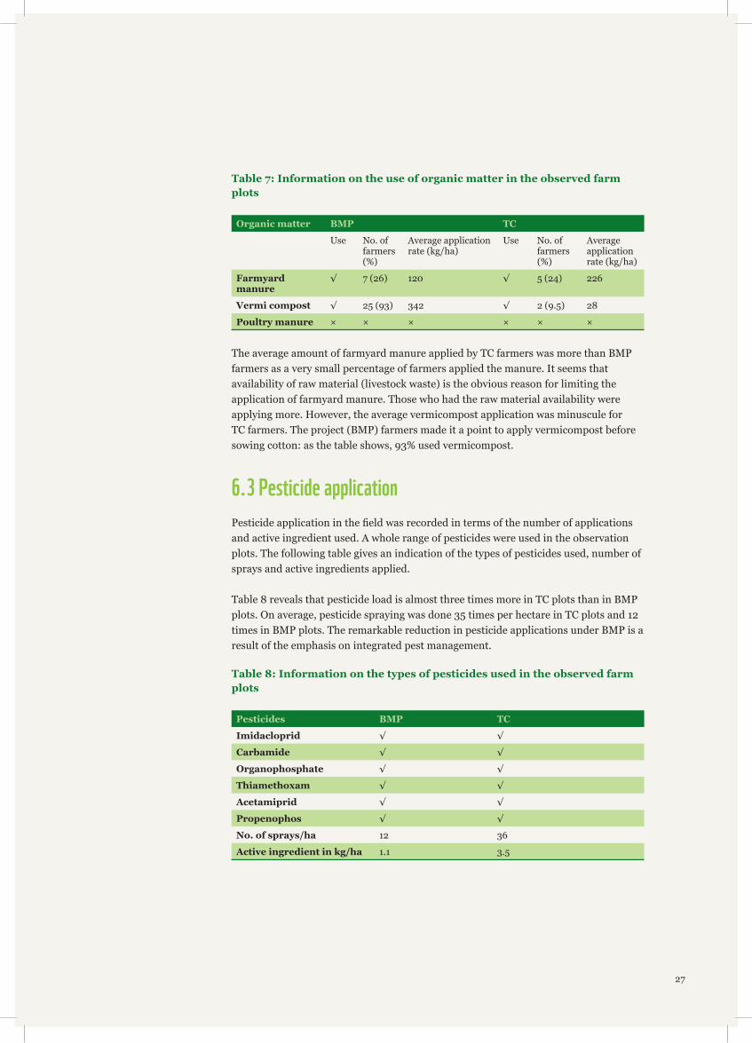
Table 7: Information on the use of organic matter in the observed farm plots

Organic matter BMP TC

Use No. of farmers (%)

Average application rate (kg/ha)

Use No. of farmers (%)

Average application rate (kg/ha)

Farmyard manure

√ 7 (26) 120 √ 5 (24) 226

Vermi compost √ 25 (93) 342 √ 2 (9.5) 28

Poultry manure × × × × × ×

The average amount of farmyard manure applied by TC farmers was more than BMP farmers as a very small percentage of farmers applied the manure. It seems that availability of raw material (livestock waste) is the obvious reason for limiting the application of farmyard manure. Those who had the raw material availability were applying more. However, the average vermicompost application was minuscule for TC farmers. The project (BMP) farmers made it a point to apply vermicompost before sowing cotton: as the table shows, 93% used vermicompost.

6.3 Pesticide application

Pesticide application in the fi eld was recorded in terms of the number of applications and active ingredient used. A whole range of pesticides were used in the observation plots. The following table gives an indication of the types of pesticides used, number of sprays and active ingredients applied.

Table 8 reveals that pesticide load is almost three times more in TC plots than in BMP plots. On average, pesticide spraying was done 35 times per hectare in TC plots and 12 times in BMP plots. The remarkable reduction in pesticide applications under BMP is a result of the emphasis on integrated pest management.

Table 8: Information on the types of pesticides used in the observed farm plots

Pesticides BMP TC

Imidacloprid √ √

Carbamide √ √

Organophosphate √ √

Thiamethoxam √ √

Acetamiprid √ √

Propenophos √ √

No. of sprays/ha 12 36

Active ingredient in kg/ha 1.1 3.5

27

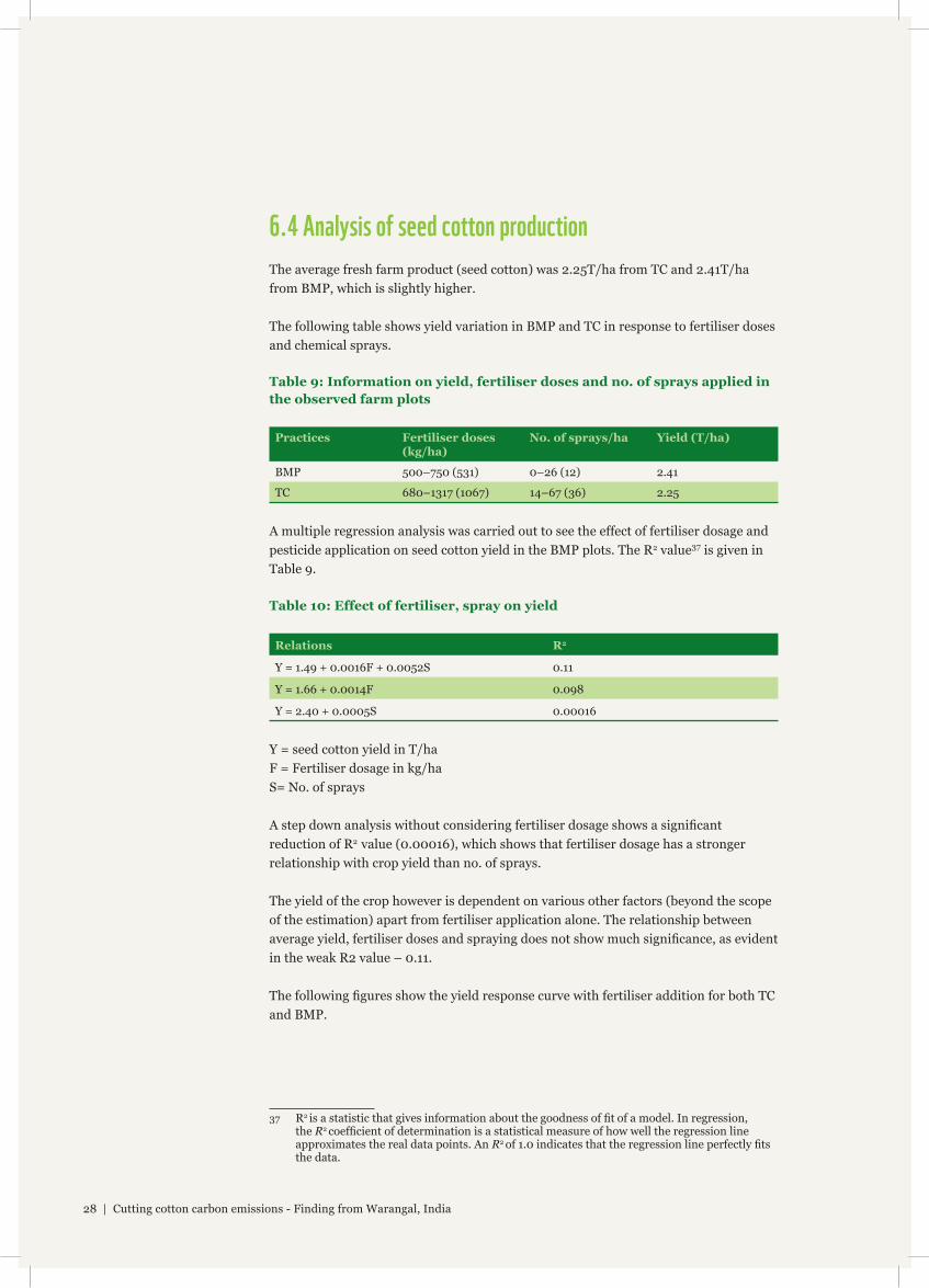
6.4 Analysis of seed cotton production

The average fresh farm product (seed cotton) was 2.25T/ha from TC and 2.41T/ha from BMP, which is slightly higher.

The following table shows yield variation in BMP and TC in response to fertiliser doses and chemical sprays.

Table 9: Information on yield, fertiliser doses and no. of sprays applied in the observed farm plots

Practices Fertiliser doses (kg/ha)

No. of sprays/ha Yield (T/ha)

BMP 500–750 (531) 0–26 (12) 2.41

TC 680–1317 (1067) 14–67 (36) 2.25

A multiple regression analysis was carried out to see the effect of fertiliser dosage and pesticide application on seed cotton yield in the BMP plots. The R2 value37 is given in Table 9.

Table 10: Effect of fertiliser, spray on yield

Relations R2

Y = 1.49 + 0.0016F + 0.0052S 0.11

Y = 1.66 + 0.0014F 0.098

Y = 2.40 + 0.0005S 0.00016

Y = seed cotton yield in T/haF = Fertiliser dosage in kg/haS= No. of sprays

A step down analysis without considering fertiliser dosage shows a signifi cant reduction of R2 value (0.00016), which shows that fertiliser dosage has a stronger relationship with crop yield than no. of sprays.

The yield of the crop however is dependent on various other factors (beyond the scope of the estimation) apart from fertiliser application alone. The relationship between average yield, fertiliser doses and spraying does not show much signifi cance, as evident in the weak R2 value – 0.11.

The following fi gures show the yield response curve with fertiliser addition for both TC and BMP.

37 R2 is a statistic that gives information about the goodness of fi t of a model. In regression, the R2 coeffi cient of determination is a statistical measure of how well the regression line approximates the real data points. An R2 of 1.0 indicates that the regression line perfectly fi ts the data.


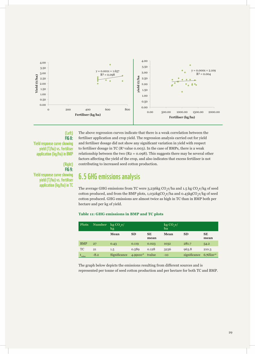
The above regression curves indicate that there is a weak correlation between the fertiliser application and crop yield. The regression analysis carried out for yield and fertiliser dosage did not show any signifi cant variation in yield with respect to fertiliser dosage in TC (R2 value 0.003). In the case of BMPs, there is a weak relationship between the two (R2 = 0.098). This suggests there may be several other factors affecting the yield of the crop, and also indicates that excess fertiliser is not contributing to increased seed cotton production.

6.5 GHG emissions analysis

The average GHG emissions from TC were 3,236kg CO2e/ha and 1.5 kg CO2e/kg of seed cotton produced, and from the BMP plots, 1,032kgCO2e/ha and 0.43kgCO2e/kg of seed cotton produced. GHG emissions are almost twice as high in TC than in BMP both per hectare and per kg of yield.

Table 11: GHG emissions in BMP and TC plots

Plots Number kg CO2e/kg

kg CO2e/ha

Mean SD SE mean

Mean SD SE mean

BMP 27 0.43 0.119 0.023 1032 281.7 54.2

TC 21 1.5 0.589 0.128 3236 963.8 210.3

tvalue -8.2 Signifi cance 4.99x10-8 tvalue -10 signifi cance 6.76X10-10

The graph below depicts the emissions resulting from different sources and is represented per tonne of seed cotton production and per hectare for both TC and BMP.

y = 0.001x + 1.657R² = 0.098

0.00

0.50

1.00

1.50

2.00

2.50

3.00

3.50

4.00

0 200 400 600 800

Yie

ld (

t/h

a)

Fertiliser (kg/ha)

9y = 0.000x + 2.10R² = 0.004

0.00

0.50

1.00

1.50

2.00

2.50

3.00

3.50

4.00

0.00 500.00 1000.00 1500.00 2000.00

yiel

d (

t/h

a

Fertiliser (kg/ha)

(Left ) FIG 8:

Yield response curve showing yield (T/ha) vs. fertiliser

application (kg/ha) in BMP

(Right) FIG 9:

Yield response curve showing yield (T/ha) vs. fertiliser application (kg/ha) in TC

29

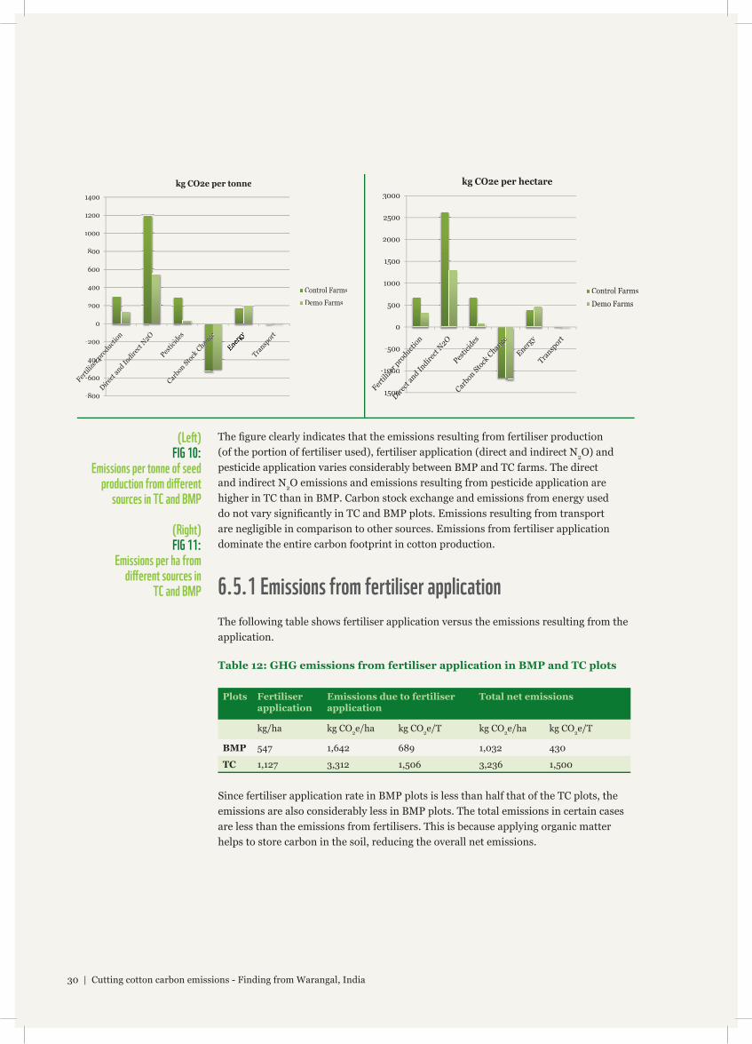
The fi gure clearly indicates that the emissions resulting from fertiliser production (of the portion of fertiliser used), fertiliser application (direct and indirect N2O) and pesticide application varies considerably between BMP and TC farms. The direct and indirect N2O emissions and emissions resulting from pesticide application are higher in TC than in BMP. Carbon stock exchange and emissions from energy used do not vary signifi cantly in TC and BMP plots. Emissions resulting from transport are negligible in comparison to other sources. Emissions from fertiliser application dominate the entire carbon footprint in cotton production.

6.5.1 Emissions from fertiliser application

The following table shows fertiliser application versus the emissions resulting from the application.

Table 12: GHG emissions from fertiliser application in BMP and TC plots

Plots Fertiliser application

Emissions due to fertiliser application

Total net emissions

kg/ha kg CO2e/ha kg CO2e/T kg CO2e/ha kg CO2e/T

BMP 547 1,642 689 1,032 430

TC 1,127 3,312 1,506 3,236 1,500

Since fertiliser application rate in BMP plots is less than half that of the TC plots, the emissions are also considerably less in BMP plots. The total emissions in certain cases are less than the emissions from fertilisers. This is because applying organic matter helps to store carbon in the soil, reducing the overall net emissions.

(Left ) FIG 10:

Emissions per tonne of seed production from diff erent

sources in TC and BMP

(Right) FIG 11:

Emissions per ha from diff erent sources in

TC and BMP

-800

-600

-400

-200

0

200

400

600

800

1000

1200

1400

kg CO2e per tonne

Control Farms

Demo Farms

-1500

-1000

-500

0

500

1000

1500

2000

2500

3000

kg CO2e per hectare

Control Farms

Demo Farms


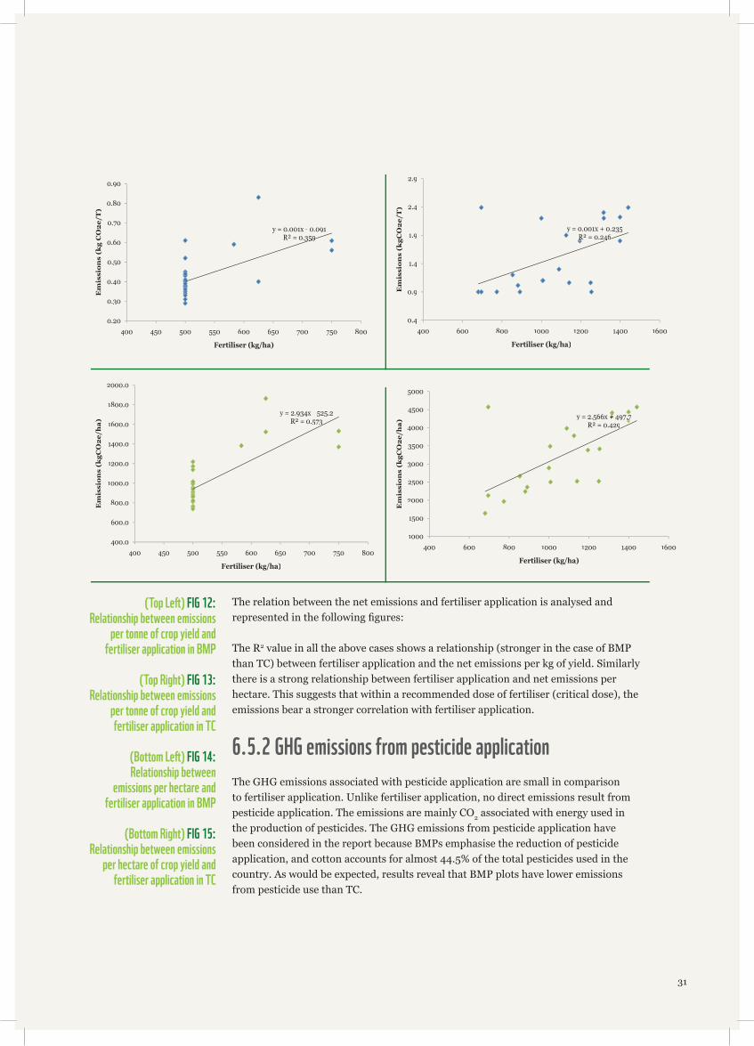
The relation between the net emissions and fertiliser application is analysed and represented in the following fi gures:

The R2 value in all the above cases shows a relationship (stronger in the case of BMP than TC) between fertiliser application and the net emissions per kg of yield. Similarly there is a strong relationship between fertiliser application and net emissions per hectare. This suggests that within a recommended dose of fertiliser (critical dose), the emissions bear a stronger correlation with fertiliser application.

6.5.2 GHG emissions from pesticide application

The GHG emissions associated with pesticide application are small in comparison to fertiliser application. Unlike fertiliser application, no direct emissions result from pesticide application. The emissions are mainly CO2 associated with energy used in the production of pesticides. The GHG emissions from pesticide application have been considered in the report because BMPs emphasise the reduction of pesticide application, and cotton accounts for almost 44.5% of the total pesticides used in the country. As would be expected, results reveal that BMP plots have lower emissions from pesticide use than TC.

y = 0.001x - 0.091R² = 0.359359

0.20

0.30

0.40

0.50

0.60

0.70

0.80

0.90

400 450 500 550 600 650 700 750 800

Em

issi

on

s (k

g C

O2

e/T

)

Fertiliser (kg/ha)

y = 2.934x - 525.2R² = 0.5733

400.0

600.0

800.0

1000.0

1200.0

1400.0

1600.0

1800.0

2000.0

400 450 500 550 600 650 700 750 800

Em

issi

on

s (k

gCO

2e/

ha

)

Fertiliser (kg/ha)

y = 0.001x + 0.235R² = 0.246RRR 46

0.4

0.9

1.4

1.9

2.4

2.9

400 600 800 1000 1200 1400 1600

Em

issi

on

s (k

gCO

2e/

T)

Fertiliser (kg/ha)

y = 2.566x + 497.7.7.77+ +++R² = 0.4299

1000

1500

2000

2500

3000

3500

4000

4500

5000

400 600 800 1000 1200 1400 1600

Em

issi

on

s (k

gCO

2e/

ha

)

Fertiliser (kg/ha)

(Top Left ) FIG 12: Relationship between emissions

per tonne of crop yield and fertiliser application in BMP

(Top Right) FIG 13: Relationship between emissions

per tonne of crop yield and fertiliser application in TC

(Bottom Left ) FIG 14: Relationship between

emissions per hectare and fertiliser application in BMP

(Bottom Right) FIG 15: Relationship between emissions

per hectare of crop yield and fertiliser application in TC

31

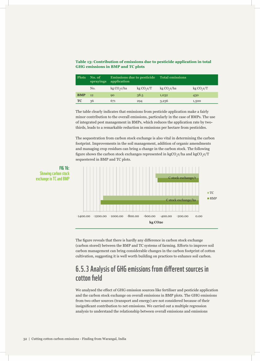
Table 13: Contribution of emissions due to pesticide application in total GHG emissions in BMP and TC plots

Plots No. of sprayings

Emissions due to pesticide application

Total emissions

No. kg CO2e/ha kg CO2e/T kg CO2e/ha kg CO2e/T

BMP 12 90 38.5 1,032 430

TC 36 671 294 3,236 1,500

The table clearly indicates that emissions from pesticide application make a fairly minor contribution to the overall emissions, particularly in the case of BMPs. The use of integrated pest management in BMPs, which reduces the application rate by two-thirds, leads to a remarkable reduction in emissions per hectare from pesticides.

The sequestration from carbon stock exchange is also vital in determining the carbon footprint. Improvements in the soil management, addition of organic amendments and managing crop residues can bring a change in the carbon stock. The following fi gure shows the carbon stock exchanges represented in kgCO2e/ha and kgCO2e/T sequestered in BMP and TC plots.

The fi gure reveals that there is hardly any difference in carbon stock exchange (carbon stored) between the BMP and TC systems of farming. Efforts to improve soil carbon management can bring considerable changes in the carbon footprint of cotton cultivation, suggesting it is well worth building on practices to enhance soil carbon.

6.5.3 Analysis of GHG emissions from diff erent sources in cotton fi eld

We analysed the effect of GHG emission sources like fertiliser and pesticide application and the carbon stock exchange on overall emissions in BMP plots. The GHG emissions from two other sources (transport and energy) are not considered because of their insignifi cant contribution to net emissions. We carried out a multiple regression analysis to understand the relationship between overall emissions and emissions

-1400.00 -1200.00 -1000.00 -800.00 -600.00 -400.00 -200.00 0.00

C stock exchange/hastock exchange/hahC stock exchange/haC stock exchange/ha

C stock exchange/tC stock exchange/t

kg CO2e

TC

BMP

FIG 16: Showing carbon stock

exchange in TC and BMP


from fertiliser, pesticide and carbon stock exchange. Table 13 shows the regression relationship as discussed above.

Table 14: Effect of nutrient application, pesticide spraying and carbon sequestration on GHG emissions in BMP and TC plots

Rl.No Regression relations R2

1 E = 861.5 + 1.11n + 0.09p + 1.46C 0.93

2 E = -898.6 + 1.13n + 0.80p 0.91

3 E = 638.69 + 1.02n + 1.08C 0.89

4 E = 4,145.38 - 0.49p + 2.58C 0.09

E = Overall emission in kg CO2e/han = emissions from fertiliser, represented as kgCO2e/hap = emissions from pesticide, represented as kgCO2e/ha

A subsequent step down analysis of each of the functions (emissions from nutrients, pesticide emissions and carbon stock exchange) is shown in Table 14. The step down process eliminates each of the variables stepwise (as seen in the multiple regression relationships) to see the change in the overall emissions due to the absence of that variable. In the regression relation (Rl. No.4), where fertiliser emissions are stepped down, there is a considerable fall of R2 value (from 0.93 to 0.09). From this, we can conclude that emissions from fertiliser are the major determinant in the overall emissions.

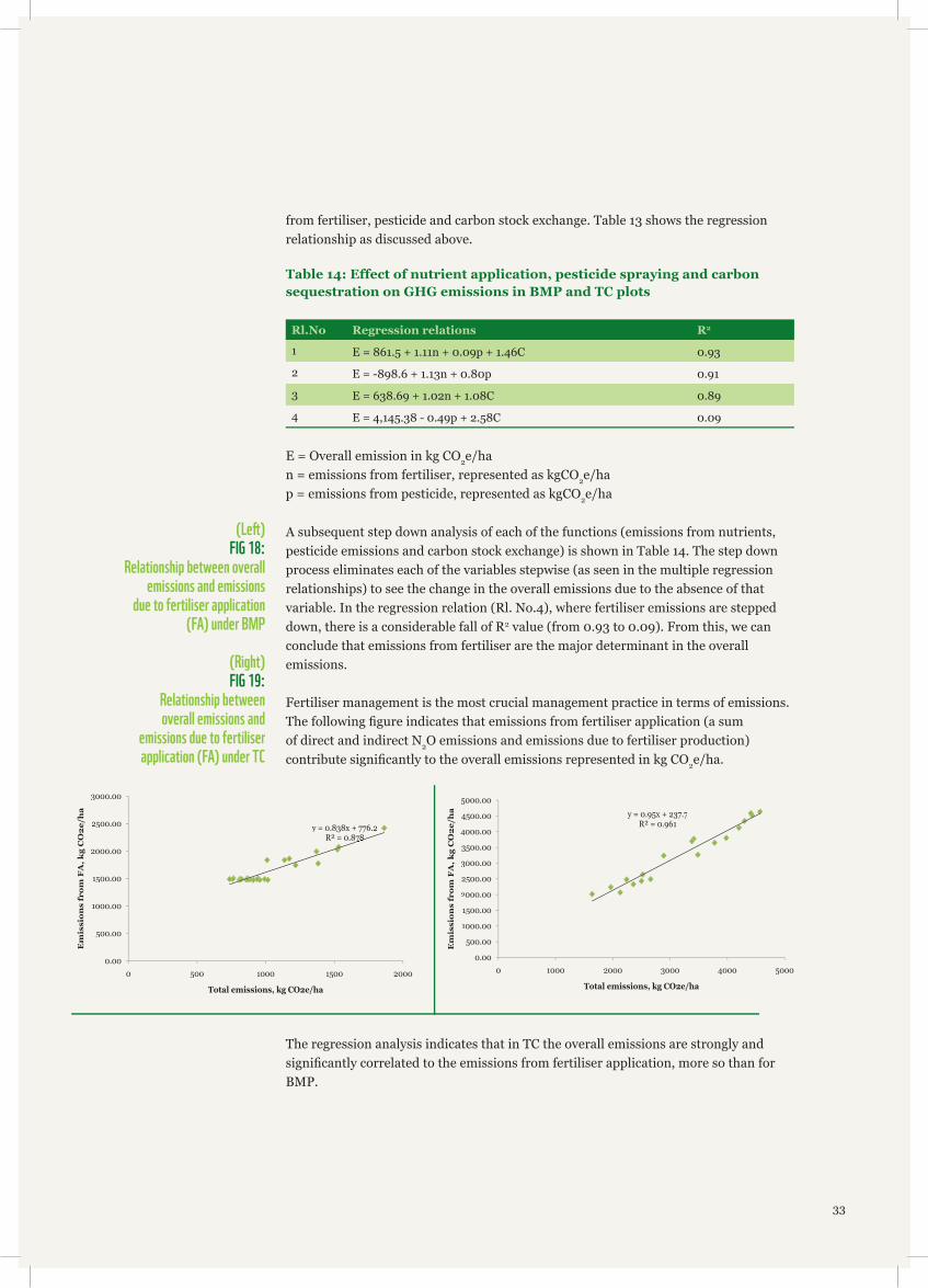
Fertiliser management is the most crucial management practice in terms of emissions. The following fi gure indicates that emissions from fertiliser application (a sum of direct and indirect N2O emissions and emissions due to fertiliser production) contribute signifi cantly to the overall emissions represented in kg CO2e/ha.

The regression analysis indicates that in TC the overall emissions are strongly and signifi cantly correlated to the emissions from fertiliser application, more so than for BMP.

y = 0.838x + 776.2R² = 0.878878

0.00

500.00

1000.00

1500.00

2000.00

2500.00

3000.00

0 500 1000 1500 2000

Em

issi

on

s fr

om

FA

, kg

CO

2e/

ha

Total emissions, kg CO2e/ha

y = 0.95x + 237.7R² = 0.961

0.00

500.00

1000.00

1500.00

2000.00

2500.00

3000.00

3500.00

4000.00

4500.00

5000.00

0 1000 2000 3000 4000 5000

Em

issi

on

s fr

om

FA

, kg

CO

2e/

ha

Total emissions, kg CO2e/ha

(Left ) FIG 18:

Relationship between overall emissions and emissions

due to fertiliser application (FA) under BMP

(Right) FIG 19:

Relationship between overall emissions and

emissions due to fertiliser application (FA) under TC

33

7.0 ConclusionThe purpose of the study was to gain an insight into the sources of GHG emissions in selected cotton fi elds using both BMPs and TC. The study found that the better managed plots emit less GHGs than traditional plots. The overall analysis suggests that the excess fertiliser application in TC is not adding to the seed cotton production but is contributing signifi cantly to GHG emissions.

As is evident from the analysis, BMPs have the potential to reduce GHG emissions in cotton fi elds. In cotton production, though the sources of GHG emissions are many (as shown in fi gures 10 and 11), fertiliser management is the major factor. Relevant emissions can be seen in both fertiliser production and fertiliser application. Emissions resulting from fertiliser production are lower in BMP than TC due to lower reliance on manufactured fertilisers; this also contributes to lower fertiliser-induced emissions (N2O). Any attempt to manage the fertiliser application will improve the reduction potential scenario.

The GHG emission estimates observed from the study in the farm plots are largely related to the inputs applied. They vary according to the changes in applied inputs within the same geographical area, so cannot be considered as defi nitive fi gures for cotton cultivation in the region. However, the results give a clear indication of the potential BMPs have to substantially reduce GHG emissions through balanced fertilisation.

We found the Cool Farm Tool invaluable for estimating the carbon footprint of cotton farming. The tool allows the user to test “what if” scenarios as it analyses the relative strength of different crop management options available. The outcome may help in developing a GHG mitigation plan for cotton production, helping to design a low-carbon, highly productive cotton system.

The following bullet points describe the possible GHG mitigation options in the present cotton context:

• Balanced fertiliser application: The analysis found that overdose of fertiliser is not adding to seed cotton yield, but is responsible for increased GHG emissions. Balanced fertiliser application at recommended dose will reduce cotton fi eld emissions.

• Crop residue management: Cotton stalk residue management was not found in the study plots during the study period because stalks are usually taken out from the fi eld and burnt. Crop residue management has the potential to sequester organic carbon in the soil and can contribute to building soil carbon stocks, reducing the carbon footprint of cotton production.

• Restricting pesticide application: Application of pesticides in plots with traditional cultivation is signifi cant, resulting in higher GHG emissions than better managed plots. Integrated pest management practices (an important component of BMP) have the potential for GHG emissions reduction.


About WWF-IndiaWWF-India is one of India’s largest conservation organizations. Established as a Charitable Trust in 1969, it has an experience of over four decades in the fi eld. Its mission is to stop the degradation of the planet’s natural environment, which it addresses through its work in biodiversity conservation and reduction of humanity’s ecological footprint.

A challenging, constructive, science-based organisation WWF addresses issues like the survival of species and habitats, climate change & energy, sustainable forest management, water resources/river basin management, sustainable agriculture and marine and freshwater Conservation. These programmes work across sectors and regions in various parts of the country. In addition to conservation of biodiversity through fi eld programmes, WWF India also aims to transform the policies and practices of key industrial sectors to reduce their ecological footprint and develop innovative sustainable solutions

© W

WF-U

K / R

EB

EC

CA

MAY

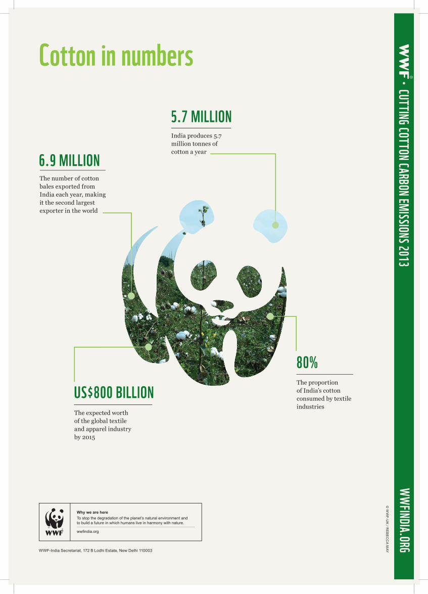
Cotton in numbers

WW

FINDIA.ORGCUTTING COTTON CARBON EM

ISSIONS 2013

6.9 MILLIONThe number of cotton bales exported from India each year, making it the second largest exporter in the world

5.7 MILLION

US$800 BILLION

80%

India produces 5.7 million tonnes of cotton a year

The expected worth of the global textile and apparel industry by 2015

The proportion of India’s cotton consumed by textile industries

WWF-India Secretariat, 172 B Lodhi Estate, New Delhi 110003

Why we are hereTo stop the degradation of the planet’s natural environment and to build a future in which humans live in harmony with nature.

Documents

WORKING TOGETHER TO DELIVER MORE SUSTAINABLE PRODUCTS ...awsassets.wwfindia.org/downloads/wwf___cotton_carbon_emission.pdf · TOGETHER TO DELIVER MORE SUSTAINABLE PRODUCTS ... .3