Worst-case evaluation complexity of regularization methods ...eprints.maths.ox.ac.uk/1874/1/NA_14_21.pdf · Worst-case evaluation complexity of regularization ... where x2IRn is the

Worst-case evaluation complexity of regularization methods

for smooth unconstrained optimization

using Holder continuous gradients

C. Cartis∗ N. I. M. Gould† and Ph. L. Toint‡

26 June 2015

Abstract

The worst-case behaviour of a general class of regularization algorithms is consideredin the case where only objective function values and associated gradient vectors are evalu-ated. Upper bounds are derived on the number of such evaluations that are needed for thealgorithm to produce an approximate first-order critical point whose accuracy is withina user-defined threshold. The analysis covers the entire range of meaningful powers inthe regularization term as well as in the Holder exponent for the gradient. The resultingcomplexity bounds vary according to the regularization power and the assumed Holderexponent, recovering known results when available.

1 Introduction

The complexity analysis of algorithms for smooth, possibly non-convex, unconstrained op-timization has been the subject of a burgeoning literature over the past few years (see thecontributions by Nesterov [12, 15], Gratton, Sartenaer and Toint [11], Cartis, Gould and Toint[3, 5, 6, 7], Ueda [17], Ueda and Yamashita[18, 19], Grapiglia, Yuan and Yuan [9, 10], andVicente [20], for instance). The present contribution belongs to this active trend and focuseson the analysis of the worst-case behaviour of regularization methods where only objectivefunction values and associated gradient vectors are evaluated. It proposes upper bounds onthe number of such evaluations that are needed for the algorithm to produce an approximatefirst-order critical point whose accuracy is within a user-defined threshold.

An analysis of this type is already available for the case where the objective function’sgradient is assumed to be Lipschitz-continuous and where the regularization uses the second orthird power of the norm of the computed step at a given iteration (see the paper by Nesterov[13] for the former and those of Cartis et al. [5, 6] for both cases). The novelty of the presentapproach is to extend the analysis to cover problems whose objective gradients are simplyHolder continuous and methods that allow weaker regularization than in the Lipschitz case.

∗Mathematical Institute, Oxford University, Oxford OX2 6GG, Great Britain. Email:[email protected]†Numerical Analysis Group, Rutherford Appleton Laboratory, Chilton OX11 0QX, Great Britain. Email:

[email protected]‡Namur Center for Complex Systems (naXys) and Department of Mathematics, University of Namur, 61,

rue de Bruxelles, B-5000 Namur, Belgium. Email: [email protected]

1

Cartis, Gould, Toint: Complexity of unconstrained optimization of C1,β functions 2

The resulting complexity bounds vary according to the regularization power and the assumedHolder exponent, providing a unified view and recovering known results when available.

The paper is organized as follows. Section 2 presents the problem and the class of algo-rithms considered. The complexity analysis itself is given in Section 3 and the sharpeness ofthe obtained result is discussed in Section 4. Section 5 finally provides some comments of theresults.

Notations: In what follows, ‖ · ‖ denotes the Euclidean norm and the T superscriptdenotes transposition. If v is a vector in IRn, [v]i denotes its i-th component.

2 The problem and algorithm

We consider the problem of finding an approximate solution of the optimization problem

minxf(x) (2.1)

where x ∈ IRn is the vector of optimization variables and f is a function from IRn into IRthat is assumed to be bounded below and continuously differentiable with Holder continuous

gradients. If we denote g(x)def= ∇xf(x), the latter says that the inequality

‖g(x)− g(y)‖ ≤ Lβ‖x− y‖β (2.2)

holds for all x, y ∈ IRn, where Lβ ≥ 0 and β > 0 are constants independent of x and y andwhere ‖ · ‖ is the Euclidean norm on IRn. As explained in Lemma 3.1 below, we will assume,without loss of generality, that β ≤ 1. Problems involving functions with Holder continuousgradients are interesting on their own rights, but can also be found in engineering practice,such as in the design of gas pipelines (the Panhandle law which governs such flows statesthat the gas flow rate in a pipeline is a power between 1 and 2 of the difference in squaredpressures, see [16, Section 17], for instance). Such functions also appear in the solution ofcertain nonlinear PDE problems (see Bensoussan and Frehse [1]).

In our context, an approximate solution for problem (2.1) is a vector xε such that

‖g(xε)‖ ≤ ε or f(x) ≤ ftarget (2.3)

where ε > 0 is a user-specified accuracy threshold and ftarget is a threshold value – independentof ε – under which the reduction of the objective function is deemed sufficient by the user.The first case in (2.3) corresponds to finding an approximate first-order-critical point. If asuitable value for ftarget is not known, minus infinity can be used instead, in effect makingthe second part of (2.3) impossible to satisfy and reducing this condition to its first part.

The class of regularization methods that we consider for computing an x satisfying (2.3)consists of iterative algorithms where, at each iteration, a local (linear or quadratic) modelof f around the current iterate xk is constructed, regularized by a term using the p-th powerof the norm of the step, and then approximately minimized (in the ”Cauchy point” sense)to provide a trial step sk. The quality of this step is then measured in order to accept theresulting trial point xk + sk as the next iterate, or to reject it and adjust the strength of theregularization.

More specifically, a regularized model of f(xk + s) of the form

mk(xk + s) = f(xk) + gTk s+ 12sTBks+

σkp‖s‖p (2.4)


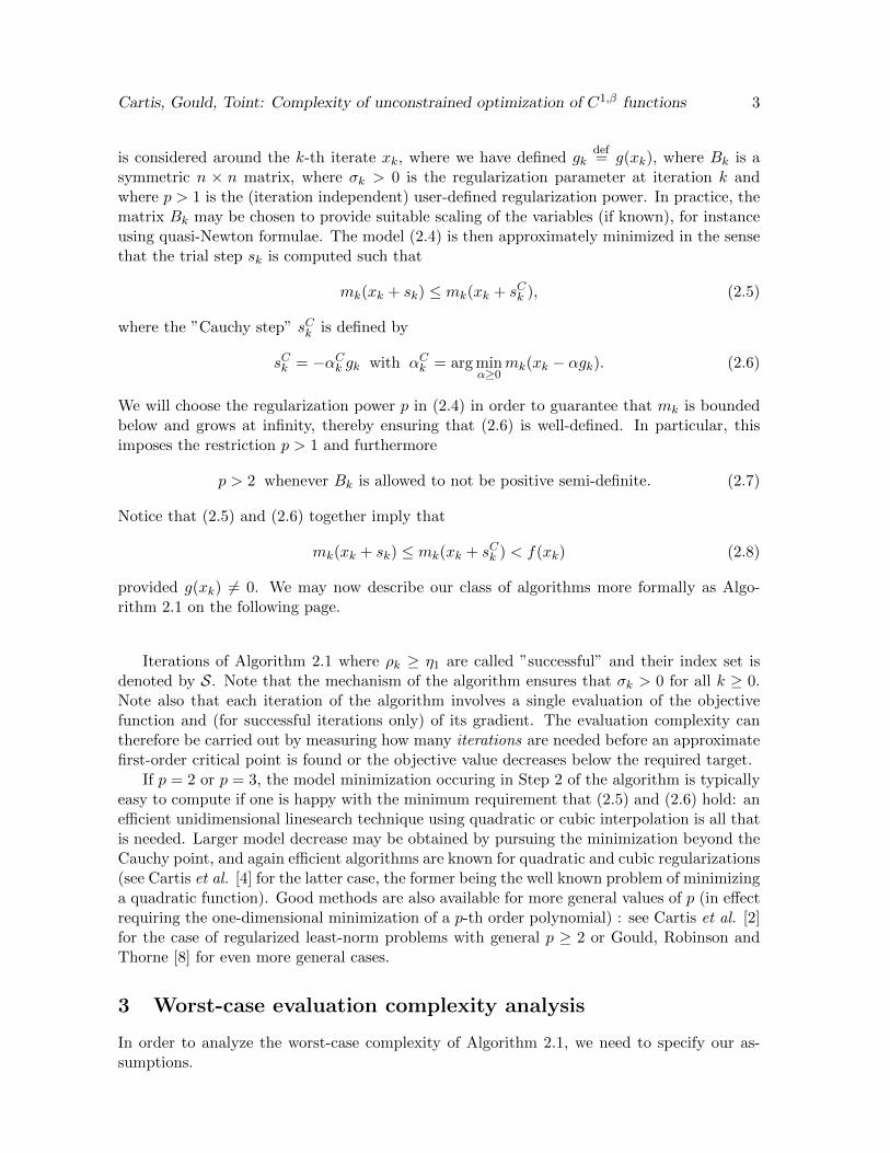
is considered around the k-th iterate xk, where we have defined gkdef= g(xk), where Bk is a

symmetric n × n matrix, where σk > 0 is the regularization parameter at iteration k andwhere p > 1 is the (iteration independent) user-defined regularization power. In practice, thematrix Bk may be chosen to provide suitable scaling of the variables (if known), for instanceusing quasi-Newton formulae. The model (2.4) is then approximately minimized in the sensethat the trial step sk is computed such that

mk(xk + sk) ≤ mk(xk + sCk ), (2.5)

where the ”Cauchy step” sCk is defined by

sCk = −αCk gk with αCk = arg minα≥0

mk(xk − αgk). (2.6)

We will choose the regularization power p in (2.4) in order to guarantee that mk is boundedbelow and grows at infinity, thereby ensuring that (2.6) is well-defined. In particular, thisimposes the restriction p > 1 and furthermore

p > 2 whenever Bk is allowed to not be positive semi-definite. (2.7)

Notice that (2.5) and (2.6) together imply that

mk(xk + sk) ≤ mk(xk + sCk ) < f(xk) (2.8)

provided g(xk) 6= 0. We may now describe our class of algorithms more formally as Algo-rithm 2.1 on the following page.

Iterations of Algorithm 2.1 where ρk ≥ η1 are called ”successful” and their index set isdenoted by S. Note that the mechanism of the algorithm ensures that σk > 0 for all k ≥ 0.Note also that each iteration of the algorithm involves a single evaluation of the objectivefunction and (for successful iterations only) of its gradient. The evaluation complexity cantherefore be carried out by measuring how many iterations are needed before an approximatefirst-order critical point is found or the objective value decreases below the required target.

If p = 2 or p = 3, the model minimization occuring in Step 2 of the algorithm is typicallyeasy to compute if one is happy with the minimum requirement that (2.5) and (2.6) hold: anefficient unidimensional linesearch technique using quadratic or cubic interpolation is all thatis needed. Larger model decrease may be obtained by pursuing the minimization beyond theCauchy point, and again efficient algorithms are known for quadratic and cubic regularizations(see Cartis et al. [4] for the latter case, the former being the well known problem of minimizinga quadratic function). Good methods are also available for more general values of p (in effectrequiring the one-dimensional minimization of a p-th order polynomial) : see Cartis et al. [2]for the case of regularized least-norm problems with general p ≥ 2 or Gould, Robinson andThorne [8] for even more general cases.

3 Worst-case evaluation complexity analysis

In order to analyze the worst-case complexity of Algorithm 2.1, we need to specify our as-sumptions.


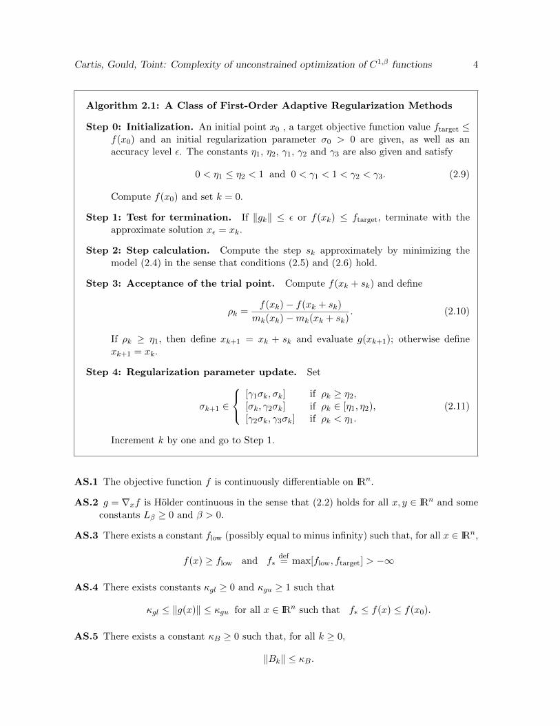
Algorithm 2.1: A Class of First-Order Adaptive Regularization Methods

Step 0: Initialization. An initial point x0 , a target objective function value ftarget ≤f(x0) and an initial regularization parameter σ0 > 0 are given, as well as anaccuracy level ε. The constants η1, η2, γ1, γ2 and γ3 are also given and satisfy

0 < η1 ≤ η2 < 1 and 0 < γ1 < 1 < γ2 < γ3. (2.9)

Compute f(x0) and set k = 0.

Step 1: Test for termination. If ‖gk‖ ≤ ε or f(xk) ≤ ftarget, terminate with theapproximate solution xε = xk.

Step 2: Step calculation. Compute the step sk approximately by minimizing themodel (2.4) in the sense that conditions (2.5) and (2.6) hold.

Step 3: Acceptance of the trial point. Compute f(xk + sk) and define

ρk =f(xk)− f(xk + sk)

mk(xk)−mk(xk + sk). (2.10)

If ρk ≥ η1, then define xk+1 = xk + sk and evaluate g(xk+1); otherwise definexk+1 = xk.

Step 4: Regularization parameter update. Set

σk+1 ∈

[γ1σk, σk] if ρk ≥ η2,[σk, γ2σk] if ρk ∈ [η1, η2),[γ2σk, γ3σk] if ρk < η1.

(2.11)

Increment k by one and go to Step 1.

AS.1 The objective function f is continuously differentiable on IRn.

AS.2 g = ∇xf is Holder continuous in the sense that (2.2) holds for all x, y ∈ IRn and someconstants Lβ ≥ 0 and β > 0.

AS.3 There exists a constant flow (possibly equal to minus infinity) such that, for all x ∈ IRn,

f(x) ≥ flow and f∗def= max[flow, ftarget] > −∞

AS.4 There exists constants κgl ≥ 0 and κgu ≥ 1 such that

κgl ≤ ‖g(x)‖ ≤ κgu for all x ∈ IRn such that f∗ ≤ f(x) ≤ f(x0).

AS.5 There exists a constant κB ≥ 0 such that, for all k ≥ 0,

‖Bk‖ ≤ κB.


AS.1 and AS.2 formalize our framework, as described in the introduction while AS.5 isstandard in similar contexts and avoids possibly infinite curvature of the model, which wouldmake the regularization irrelevant. Note that the values of Lβ ≥ 0 and β > 0 are oftenunknown to the user. AS.3 states that, if no target value is specified by the user, then theremust exist a global lower bound on the objective function’s values to make the minimizationproblem meaningful. The role of AS.4 is to take into account that, when f∗ = ftarget > flow,it may well happen that no single x ∈ IRn satisfies both conditions in (2.3), and thus that thefirst termination criterion in (2.3) cannot be satisfied by our minimization algorithm beforethe second. We take this possibility into account by allowing κgl > 0, and expresssing thecomplexity results in terms of

ε∗def= max [ ε, κgl] (3.1)

which is the ”attainable” gradient accuracy for the problem given ftarget. For simplicity ofexposition, we assume for now that ε∗ < 1, but comment on the case ε∗ ≥ 1 at the end ofthe paper. We note that AS.4 automatically holds if the set {x ∈ IRn | f∗ ≤ f(x) ≤ f(x0)} isbounded, but also, as we discuss in Lemma 3.2 below, in the frequent situation where f(x) isbounded below on the level set {x ∈ IRn | f(x) ≤ f(x0)}.

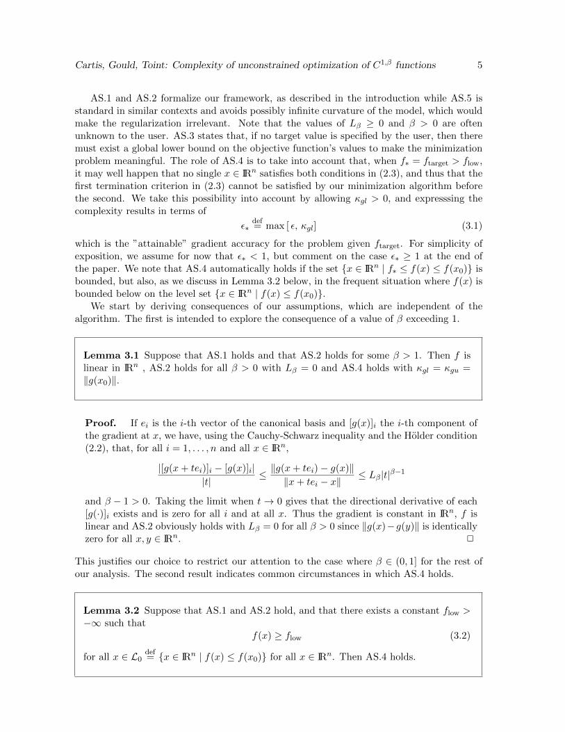
We start by deriving consequences of our assumptions, which are independent of thealgorithm. The first is intended to explore the consequence of a value of β exceeding 1.

Lemma 3.1 Suppose that AS.1 holds and that AS.2 holds for some β > 1. Then f islinear in IRn , AS.2 holds for all β > 0 with Lβ = 0 and AS.4 holds with κgl = κgu =‖g(x0)‖.

Proof. If ei is the i-th vector of the canonical basis and [g(x)]i the i-th component ofthe gradient at x, we have, using the Cauchy-Schwarz inequality and the Holder condition(2.2), that, for all i = 1, . . . , n and all x ∈ IRn,

|[g(x+ tei)]i − [g(x)]i||t|

≤ ‖g(x+ tei)− g(x)‖‖x+ tei − x‖

≤ Lβ|t|β−1

and β − 1 > 0. Taking the limit when t → 0 gives that the directional derivative of each[g(·)]i exists and is zero for all i and at all x. Thus the gradient is constant in IRn, f islinear and AS.2 obviously holds with Lβ = 0 for all β > 0 since ‖g(x)−g(y)‖ is identicallyzero for all x, y ∈ IRn. 2

This justifies our choice to restrict our attention to the case where β ∈ (0, 1] for the rest ofour analysis. The second result indicates common circumstances in which AS.4 holds.

Lemma 3.2 Suppose that AS.1 and AS.2 hold, and that there exists a constant flow >−∞ such that

f(x) ≥ flow (3.2)

for all x ∈ L0def= {x ∈ IRn | f(x) ≤ f(x0)} for all x ∈ IRn. Then AS.4 holds.


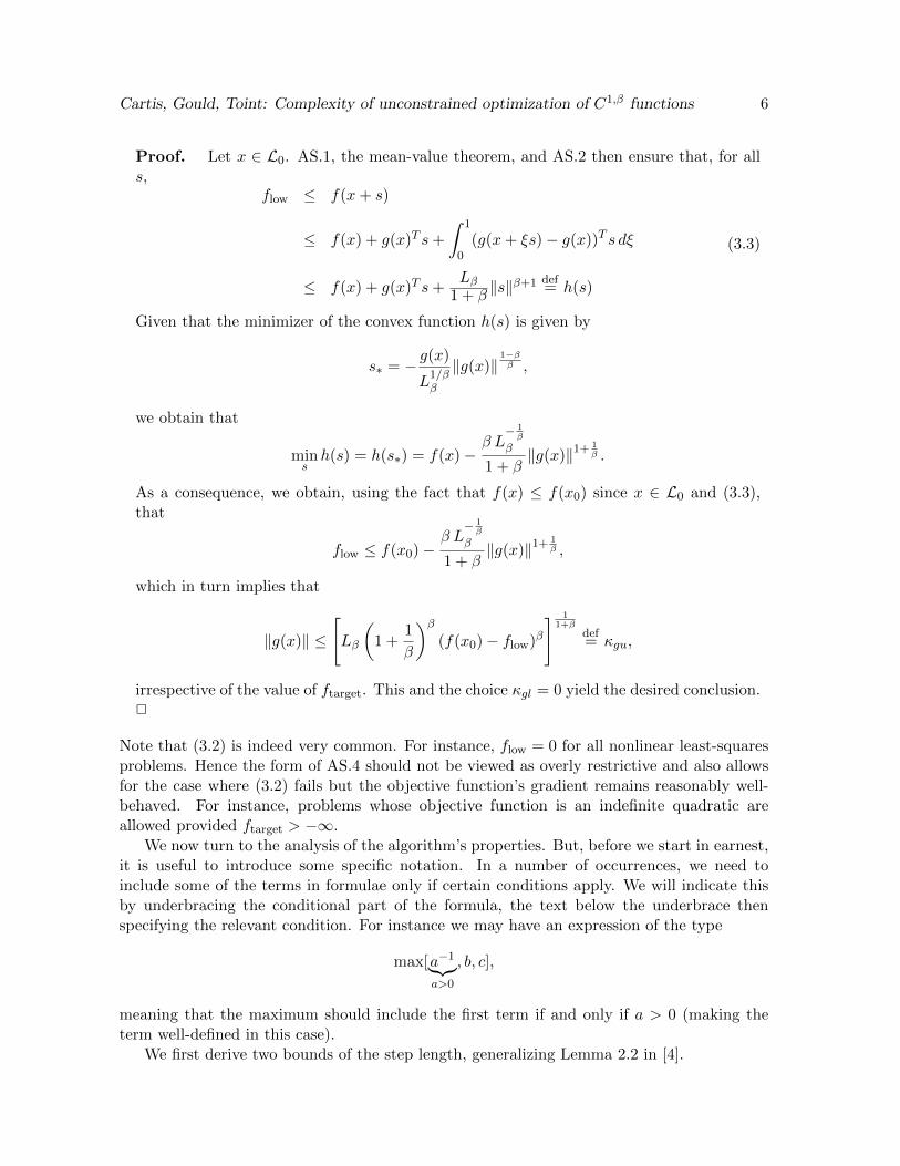
Proof. Let x ∈ L0. AS.1, the mean-value theorem, and AS.2 then ensure that, for alls,

flow ≤ f(x+ s)

≤ f(x) + g(x)T s+

∫ 1

0(g(x+ ξs)− g(x))T s dξ

≤ f(x) + g(x)T s+Lβ

1 + β‖s‖β+1 def

= h(s)

(3.3)

Given that the minimizer of the convex function h(s) is given by

s∗ = − g(x)

L1/ββ

‖g(x)‖1−ββ ,

we obtain that

minsh(s) = h(s∗) = f(x)−

β L− 1β

β

1 + β‖g(x)‖1+

1β .

As a consequence, we obtain, using the fact that f(x) ≤ f(x0) since x ∈ L0 and (3.3),that

flow ≤ f(x0)−β L− 1β

β

1 + β‖g(x)‖1+

1β ,

which in turn implies that

‖g(x)‖ ≤

[Lβ

(1 +

1

β

)β(f(x0)− flow)β

] 11+β

def= κgu,

irrespective of the value of ftarget. This and the choice κgl = 0 yield the desired conclusion.2

Note that (3.2) is indeed very common. For instance, flow = 0 for all nonlinear least-squaresproblems. Hence the form of AS.4 should not be viewed as overly restrictive and also allowsfor the case where (3.2) fails but the objective function’s gradient remains reasonably well-behaved. For instance, problems whose objective function is an indefinite quadratic areallowed provided ftarget > −∞.

We now turn to the analysis of the algorithm’s properties. But, before we start in earnest,it is useful to introduce some specific notation. In a number of occurrences, we need toinclude some of the terms in formulae only if certain conditions apply. We will indicate thisby underbracing the conditional part of the formula, the text below the underbrace thenspecifying the relevant condition. For instance we may have an expression of the type

max[a−1︸︷︷︸a>0

, b, c],

meaning that the maximum should include the first term if and only if a > 0 (making theterm well-defined in this case).

We first derive two bounds of the step length, generalizing Lemma 2.2 in [4].


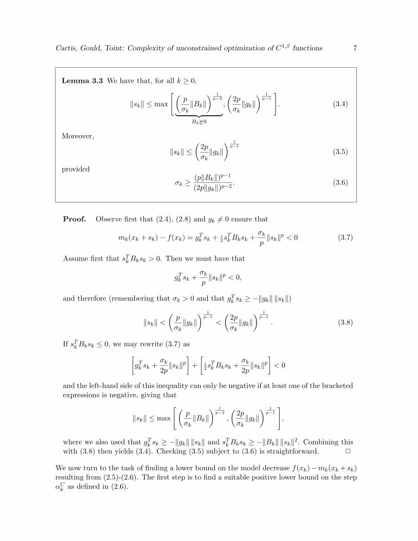
Lemma 3.3 We have that, for all k ≥ 0,

‖sk‖ ≤ max

[(p

σk‖Bk‖

) 1p−2

︸︷︷︸Bk 6�0

,

(2p

σk‖gk‖

) 1p−1

]. (3.4)

Moreover,

‖sk‖ ≤(

2p

σk‖gk‖

) 1p−1

(3.5)

provided

σk ≥(p‖Bk‖)p−1

(2p‖gk‖)p−2. (3.6)

Proof. Observe first that (2.4), (2.8) and gk 6= 0 ensure that

mk(xk + sk)− f(xk) = gTk sk + 12sTkBksk +

σkp‖sk‖p < 0 (3.7)

Assume first that sTkBksk > 0. Then we must have that

gTk sk +σkp‖sk‖p < 0,

and therefore (remembering that σk > 0 and that gTk sk ≥ −‖gk‖ ‖sk‖)

‖sk‖ <(p

σk‖gk‖

) 1p−1

<

(2p

σk‖gk‖

) 1p−1

. (3.8)

If sTkBksk ≤ 0, we may rewrite (3.7) as[gTk sk +

σk2p‖sk‖p

]+

[12sTkBksk +

σk2p‖sk‖p

]< 0

and the left-hand side of this inequality can only be negative if at least one of the bracketedexpressions is negative, giving that

‖sk‖ ≤ max

[(p

σk‖Bk‖

) 1p−2

,

(2p

σk‖gk‖

) 1p−1

],

where we also used that gTk sk ≥ −‖gk‖ ‖sk‖ and sTkBksk ≥ −‖Bk‖ ‖sk‖2. Combining thiswith (3.8) then yields (3.4). Checking (3.5) subject to (3.6) is straightforward. 2

We now turn to the task of finding a lower bound on the model decrease f(xk)−mk(xk + sk)resulting from (2.5)-(2.6). The first step is to find a suitable positive lower bound on the stepαCk as defined in (2.6).


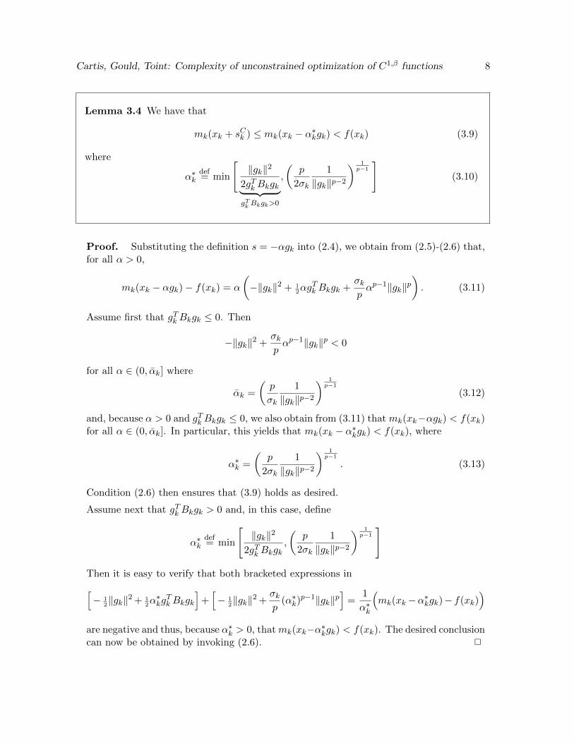
Lemma 3.4 We have that

mk(xk + sCk ) ≤ mk(xk − α∗kgk) < f(xk) (3.9)

where

α∗kdef= min

[‖gk‖2

2gTk Bkgk︸︷︷︸gTk Bkgk>0

,

(p

2σk

1

‖gk‖p−2

) 1p−1

](3.10)

Proof. Substituting the definition s = −αgk into (2.4), we obtain from (2.5)-(2.6) that,for all α > 0,

mk(xk − αgk)− f(xk) = α

(−‖gk‖2 + 1

2αgTk Bkgk +

σkpαp−1‖gk‖p

). (3.11)

Assume first that gTk Bkgk ≤ 0. Then

−‖gk‖2 +σkpαp−1‖gk‖p < 0

for all α ∈ (0, αk] where

αk =

(p

σk

1

‖gk‖p−2

) 1p−1

(3.12)

and, because α > 0 and gTk Bkgk ≤ 0, we also obtain from (3.11) that mk(xk−αgk) < f(xk)for all α ∈ (0, αk]. In particular, this yields that mk(xk − α∗kgk) < f(xk), where

α∗k =

(p

2σk

1

‖gk‖p−2

) 1p−1

. (3.13)

Condition (2.6) then ensures that (3.9) holds as desired.

Assume next that gTk Bkgk > 0 and, in this case, define

α∗kdef= min

[‖gk‖2

2gTk Bkgk,

(p

2σk

1

‖gk‖p−2

) 1p−1

]

Then it is easy to verify that both bracketed expressions in[− 1

2‖gk‖2 + 1

2α∗kg

Tk Bkgk

]+[− 1

2‖gk‖2 +

σkp

(α∗k)p−1‖gk‖p

]=

1

α∗k

(mk(xk−α∗kgk)− f(xk)

)are negative and thus, because α∗k > 0, thatmk(xk−α∗kgk) < f(xk). The desired conclusioncan now be obtained by invoking (2.6). 2


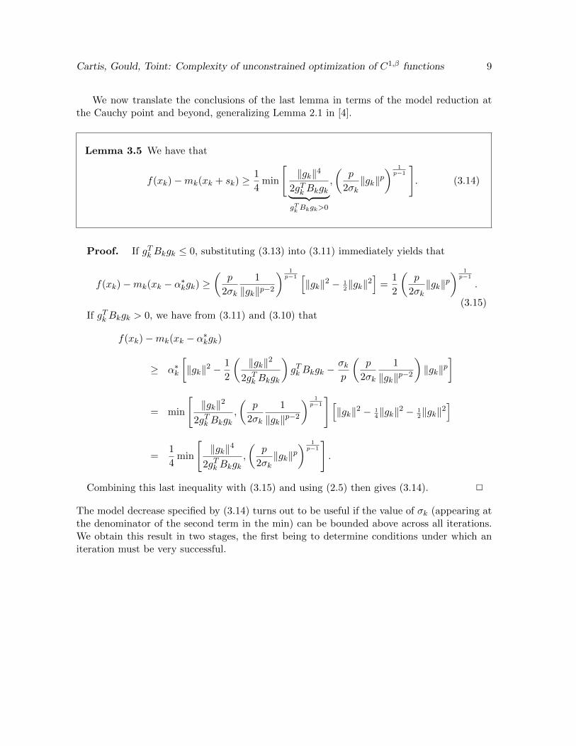
We now translate the conclusions of the last lemma in terms of the model reduction atthe Cauchy point and beyond, generalizing Lemma 2.1 in [4].

Lemma 3.5 We have that

f(xk)−mk(xk + sk) ≥1

4min

[‖gk‖4

2gTk Bkgk︸︷︷︸gTk Bkgk>0

,

(p

2σk‖gk‖p

) 1p−1

]. (3.14)

Proof. If gTk Bkgk ≤ 0, substituting (3.13) into (3.11) immediately yields that

f(xk)−mk(xk − α∗kgk) ≥(

p

2σk

1

‖gk‖p−2

) 1p−1 [

‖gk‖2 − 12‖gk‖2

]=

1

2

(p

2σk‖gk‖p

) 1p−1

.

(3.15)If gTk Bkgk > 0, we have from (3.11) and (3.10) that

f(xk)−mk(xk − α∗kgk)

≥ α∗k

[‖gk‖2 −

1

2

(‖gk‖2

2gTk Bkgk

)gTk Bkgk −

σkp

(p

2σk

1

‖gk‖p−2

)‖gk‖p

]

= min

[‖gk‖2

2gTk Bkgk,

(p

2σk

1

‖gk‖p−2

) 1p−1

] [‖gk‖2 − 1

4‖gk‖2 − 1

2‖gk‖2

]

=1

4min

[‖gk‖4

2gTk Bkgk,

(p

2σk‖gk‖p

) 1p−1

].

Combining this last inequality with (3.15) and using (2.5) then gives (3.14). 2

The model decrease specified by (3.14) turns out to be useful if the value of σk (appearing atthe denominator of the second term in the min) can be bounded above across all iterations.We obtain this result in two stages, the first being to determine conditions under which aniteration must be very successful.


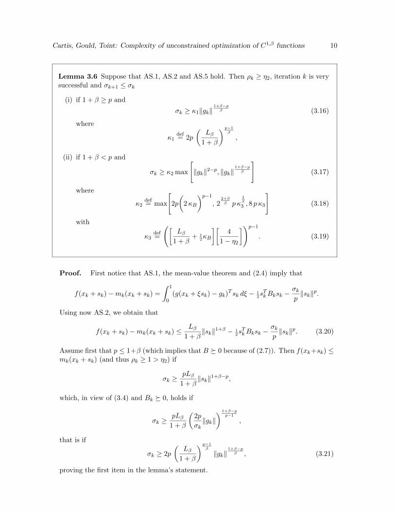
Lemma 3.6 Suppose that AS.1, AS.2 and AS.5 hold. Then ρk ≥ η2, iteration k is verysuccessful and σk+1 ≤ σk

(i) if 1 + β ≥ p and

σk ≥ κ1‖gk‖1+β−pβ (3.16)

where

κ1def= 2p

(Lβ

1 + β

) p−1β

,

(ii) if 1 + β < p and

σk ≥ κ2 max

[‖gk‖2−p, ‖gk‖

1+β−pβ

](3.17)

where

κ2def= max

[2p

(2κB

)p−1, 2

2+ββ p κ

1β

3 , 8 p κ3

](3.18)

with

κ3def=

([Lβ

1 + β+ 1

2κB

][4

1− η2

])p−1. (3.19)

Proof. First notice that AS.1, the mean-value theorem and (2.4) imply that

f(xk + sk)−mk(xk + sk) =

∫ 1

0(g(xk + ξsk)− gk)T sk dξ − 1

2sTkBksk −

σkp‖sk‖p.

Using now AS.2, we obtain that

f(xk + sk)−mk(xk + sk) ≤Lβ

1 + β‖sk‖1+β − 1

2sTkBksk −

σkp‖sk‖p. (3.20)

Assume first that p ≤ 1+β (which implies that B � 0 because of (2.7)). Then f(xk+sk) ≤mk(xk + sk) (and thus ρk ≥ 1 > η2) if

σk ≥pLβ

1 + β‖sk‖1+β−p,

which, in view of (3.4) and Bk � 0, holds if

σk ≥pLβ

1 + β

(2p

σk‖gk‖

) 1+β−pp−1

,

that is if

σk ≥ 2p

(Lβ

1 + β

) p−1β

‖gk‖1+β−pβ , (3.21)

proving the first item in the lemma’s statement.


Assume now that p > 1 + β, in which case Bk is allowed to be indefinite if p > 2 and wecannot guarantee that sTkBksk ≥ 0 in (3.20). Then ρk ≥ η2 if

rkdef= f(xk + sk)−mk(xk + sk)− (1− η2)(f(xk)−mk(xk + sk)) < 0.

Note that a lower bound on f(xk)−mk(xk+sk) is given by Lemma 3.5. If we now assumethat, whenever gTk Bkgk > 0,

σk ≥p

2(2κB)p−1 ‖gk‖2−p, (3.22)

then we obtain that the minimum occurring in the right-hand side of (3.14) is achievedby the second term, yielding that

f(xk)−mk(xk + sk) ≥1

4

(p

2σk‖gk‖p

) 1p−1

.

As a consequence, we obtain from (3.20), the Cauchy-Schwarz inequality and AS.5 that

rk ≤Lβ

1 + β‖sk‖1+β + 1

2κB‖sk‖2 −

1− η24

(p

2σk‖gk‖p

) 1p−1

.

If we also assume that, whenever Bk 6� 0, (3.6) also holds, then we may substitute theupper bound (3.5) in this equation and obtain that rk < 0 if

Lβ1 + β

(2p

σk‖gk‖

) 1+βp−1

+ 12κB

(2p

σk‖gk‖

) 2p−1

<1− η2

4

(p

2σk‖gk‖p

) 1p−1

.

Now, if, on one hand, (2p

σk‖gk‖

) 1+βp−1

≥(

2p

σk‖gk‖

) 2p−1

, (3.23)

then we obtain that rk < 0 if(Lβ

1 + β+ 1

2κB

)(2p

σk‖gk‖

) 1+βp−1

<1− η2

4

(p

2σk‖gk‖p

) 1p−1

.

Taking the (p− 1)-th power and rearranging, we obtain that rk < 0 if

σk ≥ 22+ββ p

(Lβ

1 + β+ 1

2κB

) p−1β(

4

1− η2

) p−1β

‖gk‖1+β−pβ . (3.24)

If, on the other hand, (3.23) fails, then rk < 0 if(Lβ

1 + β+ 1

2κB

)(2p

σk‖gk‖

) 2p−1

<1− η2

4

(p

2σk‖gk‖p

) 1p−1

.

Once more taking the (p− 1)-th power and rearranging, we obtain that rk < 0 if

σk ≥ 8p

(Lβ

1 + β+ 1

2κB

)p−1( 4

1− η2

)p−1‖gk‖2−p. (3.25)


Thus rk < 0 (and therefore ρk ≥ η2) when p > 1 + β provided (3.24) and (3.25) holdtogether with (3.6) (when Bk 6� 0) and (3.22) (when gTk Bkgk > 0). This proves the seconditem in the lemma’s statement if we note that

(pκB)p−1

(2p)p−2= 2p

(1

2κB

)p−1< 2p

(2κB

)p−1and

p

2(2κB)p−1 < 2p

(2κB

)p−1.

2

Note that the second part of the lemma extends the result of Lemma 3.1 in [5] to general pand β. We are now in position to prove an iteration-independent upper bound on the valueof σk.

Lemma 3.7 Suppose that AS.1–AS.5 hold and that ε∗ < 1. Then, as long as thealgorithm does not terminate, we have that, for all k ≥ 0,

(i) if 1 + β ≥ p,σk ≤ κσ1 , (3.26)

whereκσ1

def= max

[γ3κ1κ

1+β−pgu , σ0

](3.27)

(ii) if 1 + β < p,

σk ≤ max[κσ2 , κ

σ3 ε

1+β−pβ

∗

], (3.28)

where

κσ2def= max

[0, γ3κ2κ

2−pgu︸︷︷︸

p≤2

, σ0

]and κσ3

def= γ3κ2. (3.29)

with κ1 and κ2 defined in (3.18).

Proof. We again distinguish two cases. Assume first that 1 + β ≥ p, which in turnimplies that p ∈ (1, 2] and thus, in view of (2.7), that Bk � 0 for all k. Then AS.4 andcondition Lemma 3.6 (i) imply that σk+1 ≤ σk provided

σk ≥ κ1κ1+β−pβ

gu , (3.30)

which is a constant independent of k and ε.

The second case is when 1 + β < p. We first consider the subclass where p ≤ 2 where,using AS.4,

‖gk‖2−p ≤ κ2−pgu . (3.31)

This bound, part (ii) of Lemma 3.6 and the fact that ‖gk‖ > ε∗ as long as the algorithmhas not terminated then imply that σk+1 ≤ σk provided

σk ≥ κ2 max

[κ2−pgu︸︷︷︸p≤2

, ε1+β−pβ

∗

](3.32)


where we have used that 1 + β − p < 0. Alternatively, if p > 2, part (ii) of Lemma 3.6and the fact that ‖gk‖ > ε∗ as long as the algorithm has not terminated then give thatσk+1 ≤ σk provided

σk ≥ κ2 max

[ε2−p∗ , ε

1+β−pβ

∗

]= κ2ε

1+β−pβ

∗ , (3.33)

where the last equality now results from the fact that , because β ≤ 1,

0 > 2− p ≥ 2− pβ≥ 1 + β − p

β.

The proof of (3.26) and (3.28) is then completed by taking into account that the initialparameter σ0 may exceed the bound given by the right-hand side (3.30) (if 1 + β ≥ p)or (3.32) (if 1 + β < p), and also that these bounds may just fail by a small margin atan unsuccessful iteration, resulting in an increase of σk by a factor γ3 before the relevantbound applies. 2

Having now derived an iteration independent upper bound on σk, we may return to the modeldecrease given by Lemma 3.5.

Lemma 3.8 Suppose that AS.1– AS.5 hold and that ε∗ < 1. Then, as long as thealgorithm does not terminate,

• if 1 + β ≥ p, then

f(xk)−m(xk + sk) ≥ κm1 εpp−1∗ . (3.34)

where

κm1def=

1

4min

[ 1

2κB,

(p

2κσ1

) 1p−1 ]

, (3.35)

• if 1 + β < p, then

f(xk)−m(xk + sk) ≥ κm2 ε1+ 1

β∗ . (3.36)

where

κm2def=

1

4min

[ 1

2κB,

(p

2κσ2

) 1p−1 ]

. (3.37)

Proof. Assume first that 1 + β ≥ p. As above, this implies that p ∈ [1, 2] and hence,because of (2.7), that gTk Bkgk ≥ 0. Taking into account that, in this case,

gTk Bkgk ≤ κB‖gk‖2


because of AS.5, substituting (3.26) into (3.14) and using (3.26) and the fact that ‖gk‖ ≥ ε∗as long as the algorithm has not terminated, yields that

f(xk)−mk(xk + sk) ≥ 14 min

[ε2∗

2κB,

(p

2κσ1

) 1p−1

εpp−1∗

]

≥ 14 min

[1

2κB,

(p

2κσ1

) 1p−1

]min

(ε2∗, ε

pp−1∗

)and (3.34) follows since ε∗ < 1 and

p

p− 1≥ 2 for p ∈ [1, 2].

Consider now the case where 1 + β < p. Substituting now (3.28) into (3.14), using (3.28),AS.5 and the fact that ‖gk‖ ≥ ε∗ as long as the algorithm has not terminated, we obtainthat

f(xk)−mk(xk + sk) ≥ 14 min

[ε2∗

2κB︸︷︷︸gTk Bkgk>0

,

p εp∗

2 max

[κσ2 , κ

σ3 ε

1+β−pβ

∗

]

1p−1 ]

≥ 14 min

[1

2κB,

(p

2 max [κσ2 , κσ3 ]

) 1p−1

]min

(ε2∗, ε

pp−1∗ , ε

1+ 1β

∗

).

which yields (3.36) since ε∗ < 1 and, for 1 + β < p and β ∈ (0, 1],

1 +1

β≥ p

p− 1and 1 +

1

β≥ 2.

2

We now recall an important technical lemma which, in effect, gives a bound on the totalnumber of unsuccessful iterations before iteration k as a function of the number of successfulones.

Lemma 3.9 The mechanism of Algorithm 2.1 guarantees that, if

σk ≤ σmax, (3.38)

for some σmax > 0, then

k ≤ |Sk|(

1 +| log γ1|log γ2

)+

1

log γ2log

(σmax

σ0

). (3.39)

Proof. See [5]. 2


We are now ready to prove our main result on the worst-case complexity of Algorithm 2.1.

Theorem 3.10 Suppose that AS.1–AS.5 hold and that ε∗ defined in (3.1) satisfies ε∗ < 1.

1. If 1 + β ≥ p, there exist constants κsp, κap and κcp such that, for any ε > 0, Algo-

rithm 2.1 requires at most ⌊κspf(x0)− f∗

εpp−1∗

⌋(3.40)

successful iterations (and gradient evaluations),and a total of⌊κap

f(x0)− f∗

εpp−1∗

+ κcp

⌋(3.41)

iterations (and objective function evaluations) before producing an iterate xε suchthat ‖g(xε)‖ ≤ ε∗ or f(xε) ≤ ftarget.

2. If 1 + β < p, there exist constants κsβ, κaβ, κbβ and κcβ such that, for all ε > 0,Algorithm 2.1 requires at most κsβ f(x0)− f∗

ε1+ 1

β∗

(3.42)

successful iterations (and gradient evaluations) and a total ofκaβ f(x0)− f∗

ε1+ 1

β∗

+ κbβ | log ε∗|+ κcβ

(3.43)

iterations (and objective function evaluations) before producing an iterate xε suchthat ‖g(xε)‖ ≤ ε∗ or f(xε) ≤ ftarget.

In the above statements the constants are given by

κsp = κsβdef=

1

η1κm, (3.44)

κapdef=

1

η1κm

(1 +| log γ1|log γ2

), κcp

def=

1

log γ2log

(κσ1σ0

), (3.45)

κaβdef=

1

η1κm


), κbβ

def=

p− β − 1

β log γ2(3.46)

and

κcβdef=

1

log γ2

(log (max[1, κσ2 , κ

σ3 ]) + | log(σ0)|

), (3.47)


where

κ1def= 2p

(Lβ

1 + β

) p−1β

, κ2def= max

[2p

(2κB

)p−1, 2

2+ββ p κ

1β

3 , 8 p κ3

](3.48)

with

κ3def=

([Lβ

1 + β+ 1

2κB

][4

1− η2

])p−1, (3.49)

κσ1def= γ3κ1κ

1+β−pgu , κσ2

def= γ3 max

[0, κ2κ

2−pgu︸︷︷︸

p≤2

], κσ2

def= max γ3κ2. (3.50)

and

κm1def=

1

4min

[ 1

2κB,

(p

2κσ1

) 1p−1 ]

and κm2def=

1

4min

[ 1

2κB,

(p

2κσ2

) 1p−1 ]

(3.51)

Proof. Consider first the case where 1 + β ≥ p. We then deduce from AS.3, thedefinition of a successful iteration and (3.34) in Lemma 3.8, that, as long as the algorithmhas not terminated,

f(x0)− f∗ ≥ f(x0)− f(xk+1)

=∑j∈Sk

[f(xj)− f(xj + sj)

]≥ η1

∑j∈Sk

[f(xj)−mj(xj + sj)

]> η1 κm ε

pp−1∗ |Sk|,

(3.52)

where |Sk| is the cardinality of Skdef= {j ∈ S | j ≤ k}, that is the number of successful

iterations up to iteration k. This provides an upper bound on |Sk| which is independent ofk and ε∗, from which we obtain the bound (3.40) with (3.44). Calling now upon Lemma 3.9and (3.26), we deduce that the total number of iterations (and function evaluations) cannotexceed

κspf(x0)− f∗

εpp−1∗


)+

1

log γ2log

(κσ1σ0

),

which then gives the bound (3.41) with (3.45).

The proof for the case where 1+β < p is derived in a manner entirely similar to that used

for the case where 1 +β ≥ p , replacing εpp−1 by ε

1+ 1β in (3.52) since (3.34) is used instead

of (3.36), and also noting that, when using (3.28) instead of (3.26) in Lemma 3.9,

log

max[κσ2 , κ

σ3 ε

1+β−pβ

∗

]σ0

≤ ∣∣∣∣1 + β − pβ

∣∣∣∣ | log ε∗|+ log(max[1, κσ2 , κσ3 ]) + | log(σ0)|.


We may thus deduce that (3.42) and (3.43) hold with (3.46)–(3.51). 2

A close look at the expressions of the constants in (3.44)-(3.51) reveals that the global upperbound on the gradient norm, κgu, only occurs in the case where p < 2. Therefore, AS.4 isonly needed in this case since the existence of κgl ≥ 0 is always ensured by the non-negativityof ‖g(x)‖.

4 Sharpness

We now show that the bound specified by part (ii) of Theorem 3.10 is essentially sharp inthe sense that we exhibit a class of one-dimensional examples where the number of iterationsnecessary to produce an approximate first-order critical point is arbitrarily close to the the-orem’s bound(1). To achieve this goal, we first establish sequences of iterates {xk}, functionvalues {f(xk)}, gradient values {gk} and regularization parameter values {σk} which can begenerated by Algorithm 2.1 and such that the gradient values converge to zero sufficientlyslowly to attain the desired lower bound on the number of iterations (and evaluations). Oncethese are defined, we construct a function f(x) which interpolates these function and gradi-ent values and finally prove that all our assumptions are satisfied. Because the derivationof the complexity bound involves an increasing sequence of regularization parameters {σk},our example is unfortunately somewhat complicated because it has to include both success-ful and unsuccessful iterations. We choose to construct it such that all even iterations areunsuccessful and all odd ones are successful.

Consider the gradient sequence defined, for p > 1 + β, any arbitrarily small τ ∈ (0, 1), apositive integer q and all k ≥ 0, by

g2k = −(

1

k + q

) β1+β

+τ

, g2k+1 = g2k. (4.1)

and observe that the sequence of gradient norms {‖gk‖} is non-increasing for any choice of q.Assume first that q = 1. This definition implies that

|g2k+3||g2k+1|

→ 1 (4.2)

when k tends to infinity, and thus that

ω2k−1def=

(|g2k+1|

1β

|g2k+1|1β + 1

2|g2k+3|

1β

)p−1(|g2k|

1β

|g2k−1|1β

)1+β−p

→(

2

3

)p−1. (4.3)

Hence, there exists an integer ` ≥ 2 such that

ω2k−1 ∈

[1

2

(2

3

)p−1,

(5

6

)p−1]⊂ (0, 1) for k ≥ `. (4.4)

We now (re)define q in (4.1) by setting q = `, in effect shifting the {k} sequence by ` suchthat (4.2)-(4.4) holds with (4.1) for the complete shifted sequence. Note that q only depends

(1)Whether this can also be achieved for part (i) of the theorem is still unknown at this point.


on β and τ and is independent of ε. Observe also that the rate of (monotonic) convergenceof the sequence {gk} to zero ensures that, for any ε ∈ (0, 1), |gk| ≤ ε only for k larger than

2(bε−1+β

β+τ(1+β) c − q).In order to ensure the proper rate of increase of σk, we choose to set

σ2k+1 = |g2k+1|1+β−pβ (4.5)

for all k ≥ 0 (remembering that odd iterations are successful), while the value of σ2k is still tobe determined within the constraints of (2.11). Associated with the sequence {gk}, we definethe sequence of iterates {xk} by

x0 = x1 = 0, x2k+2 = x2k+1 + s2k+1 = x2k+3 (k ≥ 0).

In this definition, the step s2k+1 at a successful iterations is computed by minimizing themodel (2.4) with B2k+1 = 0, that is

m2k+1(x2k+1 + s) = f(x2k+1) + g2k+1 s+σ2k+1

p|s|p,

over s, where the function value f(x2k+1) is still to be defined. A simple calculation showsthat

s2k+1 =

(|g2k+1|σ2k+1

) 1p−1

= |g2k+1|1β ≤ |g0|

1β < 1, (4.6)

where we substituted (4.5) to obtain the last equality, and that

∆m2k+1def= m2k+1(x2k+1)−m2k+1(x2k+1 + s2k+1)

=(

1− 1p

)|g2k+1|

1+ββ

=(

1− 1p

)|g2k+1s2k+1|.

(4.7)

Similarly, we also define the step s2k as the minimizer of m2k(x2k + s) with B2k = 0, yielding

s2k =

(|g2k|σ2k

) 1p−1

(4.8)

and

∆m2kdef= m2k(x2k)−m2k(x2k + s2k) =

(1− 1

p

)(|g2k|p

σ2k

) 1p−1

=

(1− 1

p

)|g2ks2k|. (4.9)

The sequence of function values is then defined by

f(x0) = f(x1) = 0, f(x2k+2) = m2k+1(x2k+1 + s2k+1) = f(x2k+3) (k ≥ 0), (4.10)

where the second part guarantees the very successful nature of iteration 2k + 1. We observethat, for k ≥ 0,

f(x2k)− f(x2k+1) = 0


since iteration 2k is unsuccessful, and

f(x2k+1)− f(x2k+2) = ∆m2k+1 =

(1− 1

p

)|g2k+1|

1+ββ , (4.11)

yielding that, for every k ≥ 0, that

f(x0)− f(x2k+2) =k∑j=0

[f(x2j+1)− f(x2j+2)]

=(

1− 1p

) k∑j=0

|g2j+1|1+ββ

=(

1− 1p

) k∑j=0

(1

j + q

)1+ 1+ββτ

.

Hence the sequence {f(xk)} is bounded below by

f∞def=

(1− 1

p

)−ζ (1 +1 + β

βτ

)+

q−1∑j=1

(1

j

)1+ 1+ββτ > −∞, (4.12)

where ζ(·) is the Riemann zeta function. We conclude the definition of the sequences involvedin our example by selecting σ2k in order to impose that, for all k ≥ 0,

s2k = s2k+1 + 12s2k+3 (4.13)

where 12∈ [ 1

2, 1) is chosen as when defining q above. Using (4.8), this is equivalent to asking

that|g2k|σ2k

= (s2k+1 + 12s2k+3)

p−1 ,

which, in view of (4.5), is equivalent to requiring that

σ2kσ2k−1

=|g2k|

|g2k−1|1+β−pβ

(1

s2k+1 + 12s2k+3

)p−1.

If we now take (4.6), (4.3) and (4.4) into account, this amounts to imposing that

σ2kσ2k−1

= ω2k−1 ∈

[1

2

(2

3

)p−1,

(5

6

)p−1],

therefore satisfying (2.11) at successful iterations for a choice of γ1 ≤ 12

(23

)p−1. (In order to

start the recursion, we (arbitrarily) define σ−1 by (4.5) with k = −1 and g−1 = −[1/(q −1)]

β1+β

+τ.) We also observe that, for large enough k,

σ2k+1

σ2k=|g2k+1|

1+β−pβ

ω2k−1σ2k−1=

(s2k+1 + 1

2s2k+3

s2k+1

)p−1∈

[(s1 + 1

2s3

s1

)p−1,

(3

2

)p−1](4.14)

and (2.11) therefore also holds at unsuccessful iterations. As a consequence of this somewhatlengthy description, we may therefore deduce that the sequences {xk}, {gk} {σk} and {f(xk)}


may be generated by Algorithm 2.1 provided only that iteration 2k is indeed unsuccessful,that is if

f(x2k)− f(x2k + s2k) < η1∆m2k,

where f(x2k+s2k) is the still undefined value of our putative objective function at x2k+s2k =x2k+3+ 1

2s2k+3. This condition is obviously satisfied if we also impose that f(x2k+3+ 1

2s2k+3) =

f2k2k+3, where

f2k2k+3def= max[ f(x2k+3), f(x2k)− 0.99 η1∆m2k, f(x2k+4)− 1

2g2k+4s2k+3 ]. (4.15)

Note that this last condition ensures that

f(x2k+2) = f(x2k+3) ≤ f2k2k+3. (4.16)

and also, since f(x2k) = f(x2k+1) > f(x2k+3), that

f2k2k+3 ≥ f(x2k+4)− 12g2k+4s2k+3 ⇒ f2k2k+3 ∈ [f(x2k+3), f(x2k+1)]. (4.17)

We now turn to the definition of the objective function f(x) which must interpolatefunction and gradient values at the iterates. We start by noting that, for arbitrary a > 0 ands > 0, function values fa and fb and gradient values ga and gb, it is possible to construct afunction

fas(t) = fa + gat+ cas [sin(φast)]1+β (4.18)

on the interval [a, a + s] where the parameters cas and φas ∈ (0, π] can be determined toensure that

fas(0) = fa, gas(0) = ga, fa(s) = fb and gas(s) = gb.

Indeed, sincegas(t) = ga + cas(1 + β)φas [sin(φast)]

β cos(φast), (4.19)

we deduce thatgb − ga = cas(1 + β)φas [sin(φass)]

β cos(φass), (4.20)

which may substitute in (4.18) to obtain that

fb − fa = gas+(gb − ga) sin(φass)

(1 + β)φas cos(φass),

and hence conclude that φass is the smallest positive root θas of the nonlinear equation

sin(θ)

θ= νas cos(θ), where νas = (1 + β)

fb − fa − gas(gb − ga)s

. (4.21)

It is easy to check that such a root always exist in (0, π2 ] if νas > 1. Given φas, or, equivalently,θas = φass, we also obtain that

cas =fb − fa − gas

[sin(θas)]1+β

.

We now use this interpolation technique on each of the sequence of intervals specified inTable 4.2. Observe that the function is interpolated for every successful step in two pieces withan intermediate point corresponding (for all iterations beyond the first) to the penultimate


unsuccessful trial point, where condition (4.15) is imposed as well as a zero gradient. We alsochoose (arbitrarily)

f−21 = |g−1|(1+β)/β − 0.993η12

(|g−1|p

σ−1

)1/(p−1)

(corresponding to a fictitious unsuccessful iteration of index k = −2 with g−2 = g−1 andσ−2 = σ−1/(1 + 1

2)p−1).

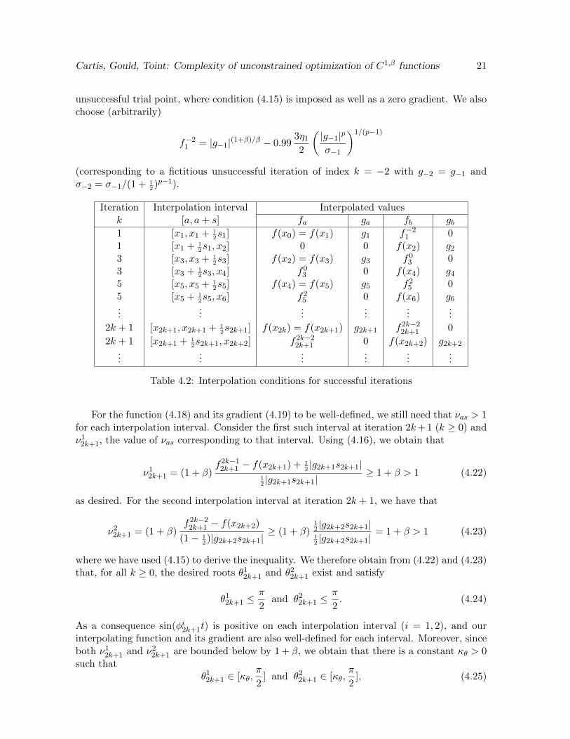
Iteration Interpolation interval Interpolated valuesk [a, a+ s] fa ga fb gb1 [x1, x1 + 1

2s1] f(x0) = f(x1) g1 f−21 0

1 [x1 + 12s1, x2] 0 0 f(x2) g2

3 [x3, x3 + 12s3] f(x2) = f(x3) g3 f03 0

3 [x3 + 12s3, x4] f03 0 f(x4) g4

5 [x5, x5 + 12s5] f(x4) = f(x5) g5 f25 0

5 [x5 + 12s5, x6] f25 0 f(x6) g6

......

......

......

2k + 1 [x2k+1, x2k+1 + 12s2k+1] f(x2k) = f(x2k+1) g2k+1 f2k−22k+1 0

2k + 1 [x2k+1 + 12s2k+1, x2k+2] f2k−22k+1 0 f(x2k+2) g2k+2

......

......

......

Table 4.2: Interpolation conditions for successful iterations

For the function (4.18) and its gradient (4.19) to be well-defined, we still need that νas > 1for each interpolation interval. Consider the first such interval at iteration 2k+ 1 (k ≥ 0) andν12k+1, the value of νas corresponding to that interval. Using (4.16), we obtain that

ν12k+1 = (1 + β)f2k−12k+1 − f(x2k+1) + 1

2|g2k+1s2k+1|

12|g2k+1s2k+1|

≥ 1 + β > 1 (4.22)

as desired. For the second interpolation interval at iteration 2k + 1, we have that

ν22k+1 = (1 + β)f2k−22k+1 − f(x2k+2)

(1− 12)|g2k+2s2k+1|

≥ (1 + β)12|g2k+2s2k+1|

12|g2k+2s2k+1|

= 1 + β > 1 (4.23)

where we have used (4.15) to derive the inequality. We therefore obtain from (4.22) and (4.23)that, for all k ≥ 0, the desired roots θ12k+1 and θ22k+1 exist and satisfy

θ12k+1 ≤π

2and θ22k+1 ≤

π

2. (4.24)

As a consequence sin(φi2k+1t) is positive on each interpolation interval (i = 1, 2), and ourinterpolating function and its gradient are also well-defined for each interval. Moreover, sinceboth ν12k+1 and ν22k+1 are bounded below by 1 + β, we obtain that there is a constant κθ > 0such that

θ12k+1 ∈ [κθ,π

2] and θ22k+1 ∈ [κθ,

π

2], (4.25)


and thus that there exists a constant κsin > 0 independent of k such that

sin(θ12k+1) ≥ κsin and sin(θ22k+1) ≥ κsin. (4.26)

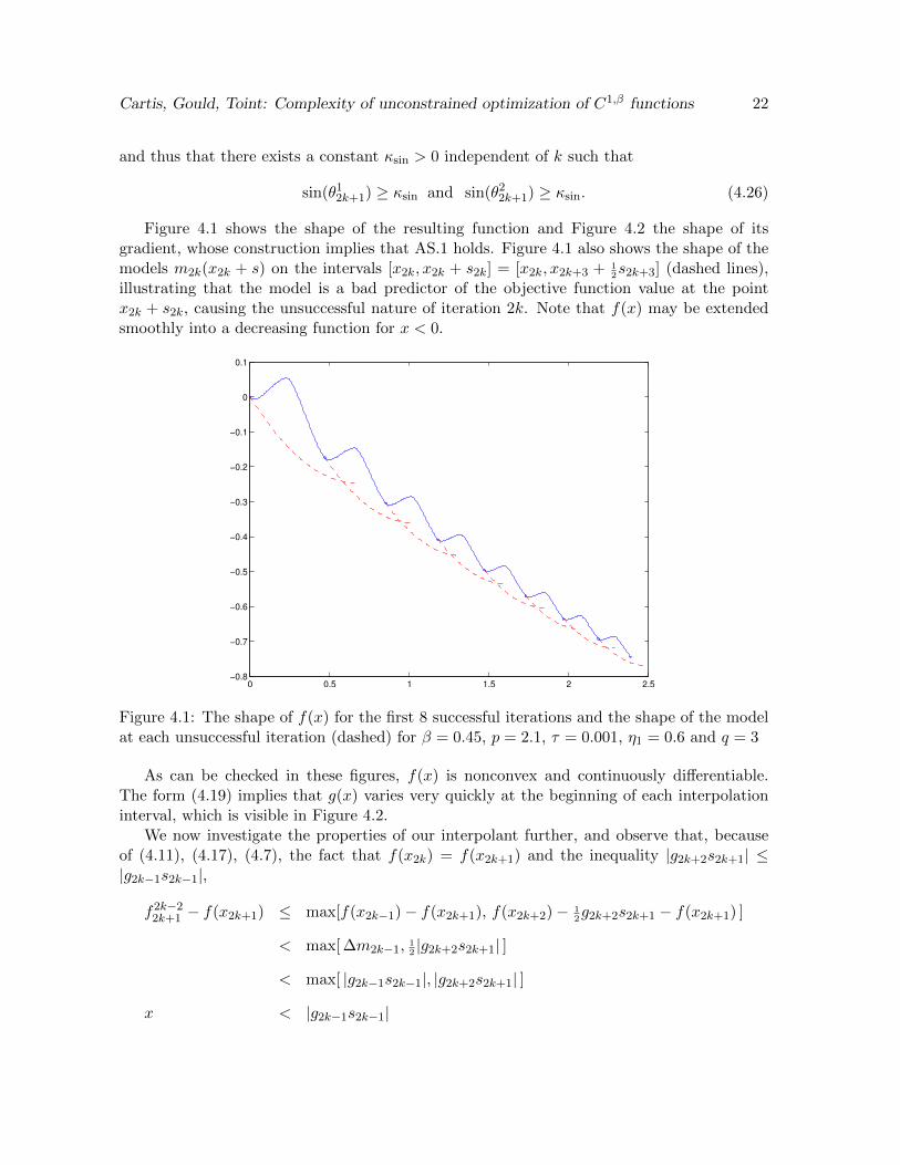
Figure 4.1 shows the shape of the resulting function and Figure 4.2 the shape of itsgradient, whose construction implies that AS.1 holds. Figure 4.1 also shows the shape of themodels m2k(x2k + s) on the intervals [x2k, x2k + s2k] = [x2k, x2k+3 + 1

2s2k+3] (dashed lines),

illustrating that the model is a bad predictor of the objective function value at the pointx2k + s2k, causing the unsuccessful nature of iteration 2k. Note that f(x) may be extendedsmoothly into a decreasing function for x < 0.

0 0.5 1 1.5 2 2.5−0.8

−0.7

−0.6

−0.5

−0.4

−0.3

−0.2

−0.1

0

0.1

Figure 4.1: The shape of f(x) for the first 8 successful iterations and the shape of the modelat each unsuccessful iteration (dashed) for β = 0.45, p = 2.1, τ = 0.001, η1 = 0.6 and q = 3

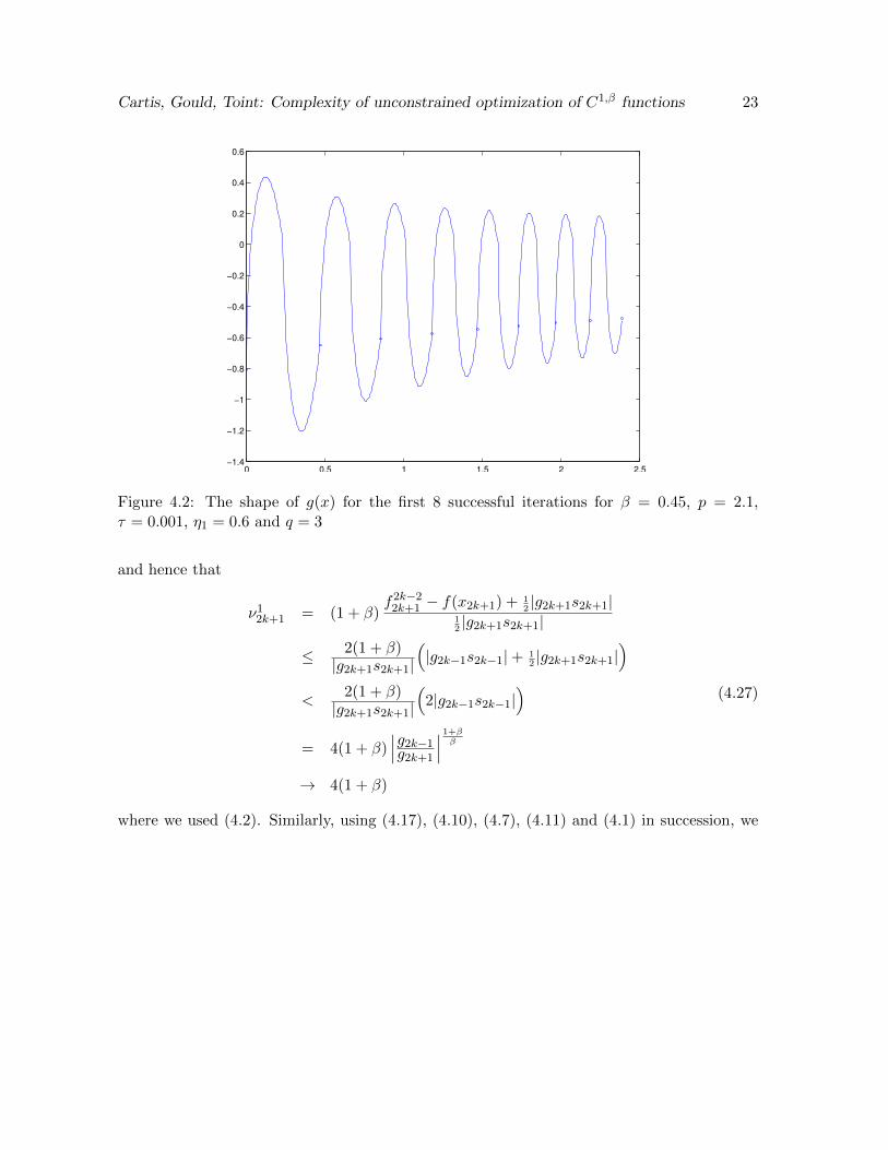
As can be checked in these figures, f(x) is nonconvex and continuously differentiable.The form (4.19) implies that g(x) varies very quickly at the beginning of each interpolationinterval, which is visible in Figure 4.2.

We now investigate the properties of our interpolant further, and observe that, becauseof (4.11), (4.17), (4.7), the fact that f(x2k) = f(x2k+1) and the inequality |g2k+2s2k+1| ≤|g2k−1s2k−1|,

f2k−22k+1 − f(x2k+1) ≤ max[f(x2k−1)− f(x2k+1), f(x2k+2)− 12g2k+2s2k+1 − f(x2k+1) ]

< max[ ∆m2k−1, 12|g2k+2s2k+1| ]

< max[ |g2k−1s2k−1|, |g2k+2s2k+1| ]

x < |g2k−1s2k−1|


0 0.5 1 1.5 2 2.5−1.4

−1.2

−1

−0.8

−0.6

−0.4

−0.2

0

0.2

0.4

0.6

Figure 4.2: The shape of g(x) for the first 8 successful iterations for β = 0.45, p = 2.1,τ = 0.001, η1 = 0.6 and q = 3

and hence that

ν12k+1 = (1 + β)f2k−22k+1 − f(x2k+1) + 1

2|g2k+1s2k+1|

12|g2k+1s2k+1|

≤ 2(1 + β)|g2k+1s2k+1|

(|g2k−1s2k−1|+ 1

2|g2k+1s2k+1|

)<

2(1 + β)|g2k+1s2k+1|

(2|g2k−1s2k−1|

)= 4(1 + β)

∣∣∣g2k−1g2k+1

∣∣∣ 1+ββ→ 4(1 + β)

(4.27)

where we used (4.2). Similarly, using (4.17), (4.10), (4.7), (4.11) and (4.1) in succession, we


obtain that

ν22k+1 = (1 + β)f2k−22k+1 − f(x2k+2)

12|g2k+2s2k+1|

≤ 2(1 + β) max[ f(x2k−1)− f(x2k+2), 12|g2k+2s2k+1| ]

|g2k+2s2k+1|

≤ 2(1 + β) max[ ∆m2k−1 + ∆m2k+1, 12|g2k+2s2k+1| ]

|g2k+2s2k+1|

≤ 2(1 + β) max

[2∆m2k−1|g2k+2s2k+1|

, 12

]= 2(1 + β) max

[2(

1− 1p

)∆m2k−1∆m2k+1

|g2k+1s2k+1||g2k+2s2k+1|

, 12

]= 2(1 + β) max

[2(

1− 1p

) ∣∣∣g2k−1g2k+1

∣∣∣ 1+ββ |g2k+1s2k+1||g2k+2s2k+1|

, 12

]= 2(1 + β) max

[2(

1− 1p

) ∣∣∣g2k−1g2k+1

∣∣∣ 1+ββ |g2k+1||g2k+2|

, 12

]→ 2(1 + β) max

[2(

1− 1p

), 12

].

(4.28)

We may therefore deduce from (4.27) and (4.28) that there exists a constant κν > 0 indepen-dent of k such that, for all k ≥ 0,

ν12k+1 ≤ κν and ν22k+1 ≤ κν .

As a consequence, and since the nonlinear equation in (4.21) can be written in the form

tan(θ) = νasθ,

we obtain that θas is uniformly bounded away from π2 and hence that there exists a constant

κcos > 0 such thatcos(θas) = cos(φass) ≥ κcos (4.29)

for every interpolation interval.Consider now 0 ≤ t1 < t2 ≤ s for a given interpolation interval [a, a + s]. Because of

(4.24), we then have that

|g(t2)− g(t1)| = |cas|(1 + β)φas{∣∣[sin(φast2)]

β cos(φast2)− [sin(φast1)]β cos(φast1)

∣∣}≤ |cas|(1 + β)φas

{∣∣[sin(φast2)]β cos(φast2)− [sin(φast2)]

β cos(φast1)∣∣

+∣∣[sin(φast2)]

β cos(φast1)− [sin(φast1)]β cos(φast1)

∣∣}= |cas|(1 + β)φas

{∣∣[sin(φast2)]β∣∣ |cos(φast2)− cos(φast1)|

+ |cos(φast1)|∣∣[sin(φast2)]

β − [sin(φast1)]β∣∣}

≤ |cas|(1 + β)φas{|cos(φast2)− cos(φast1)|+

∣∣[sin(φast2)]β − [sin(φast1)]

β∣∣}

Now, using the mean-value theorem,

|cos(φast2)− cos(φast1)| = |sin(ξ)| φas|t2 − t1| ≤(π

2

)1−βφβas|t2 − t1|β (4.30)


where ξ ∈ (φast1, φast2) and where we have used the fact

φas|t2 − t1| =π

2

(2φas|t2 − t1|

π

)≤ π

2

(2φas|t2 − t1|

π

)β.

because φas|t2 − t1| ≤ φass ≤ π2 . Moreover, using the inequality

|uβ − vβ| ≤ |u− v|β for all u, v ∈ [0, 1], (4.31)

and the fact that

sin

(φas2

(t2 − t1))<φas2

(t2 − t1)

since φas(t2 − t1) ≤ φass ≤ π2 , we deduce that∣∣[sin(φast2)]

β − [sin(φast1)]β∣∣ ≤ |sin(φast2)− sin(φast1)|β

= 2β∣∣∣cos

(φas2 (t2 + t1)

)∣∣∣β ∣∣∣sin(φas2 (t2 − t1))∣∣∣β

≤ 2β∣∣∣sin(φas2 (t2 − t1)

)∣∣∣β< φβas|t2 − t1|β.

Thus, combining this inequality with (4.30), we obtain that

|g(t2)− g(t1)| ≤[(π

2

)1−β+ 1

](1 + β) |cas|φ1+βas |t2 − t1|β. (4.32)

But we know from (4.6) that, for all k ≥ 0,

|g2k+1| = sβ2k+1 and |g2k+2| = |g2k+3| = sβ2k+1

|g2k+3||g2k+1|

≤ sβ2k+1.

As a consequence, we deduce using Table 4.2 that, for every interpolation interval,

|gb − ga| ≤ 2βsβ

because the length s of each interval is equal to half that of the corresponding successful step.Using this inequality and (4.20), we obtain that

|cas|φ1+βas ≤ φβas|gb − ga|(1 + β)[sin(θs)]

β cos(θs)

≤ 2βφβassβ

(1 + β)[sin(θs)]β cos(θs)

≤(π2

)β 2β

(1 + β)[κsin]βκcos

(4.33)

where we used the equality φass = θas, (4.24), (4.26), and (4.29) to derive the last inequality.Hence, we deduce from (4.32) that, for x and y belonging to the same interpolation interval,

|g(x)− g(y)| ≤[π

2+(π

2

)β] 2β

[κsin]βκcos|x− y|β def

= 12Lβ|x− y|β. (4.34)


Consider now 0 ≤ x < y where x and y belong to different interpolation intervals andassume first that y belongs to the interpolation interval following that containing x. Then, ifz ∈ (x, y) is the junction point between the two successive intervals,

|g(x)− g(y)| ≤ |g(x)− g(z)|+ |g(z)− g(y)|≤ 1

2Lβ|x− z|β + 1

2Lβ|z − y|β

≤ Lβ|x− y|β(4.35)

where we use the triangle inequality, (4.34) on each interval, and the fact that uβ + vβ ≤2(u+ v)β for all u, v ∈ [0, 1].

Consider finally 0 ≤ x < y where x and y belong to different interpolation intervals, wherey does not belong to the interval following that containing x. Let us denote by rx the smallestroot of g larger than x and by ry the largest root smaller than y. Note that the existence ofthese roots is guaranteed by the construction of the interpolating function f which ensuresthat stationary point occurs at the junction between to two interpolation intervals coveringa single successful step. It is easy to verify that x and rx must belong either to the sameinterpolation interval or to two successive intervals. The same is true of ry and y, yieldingthat

|x− rx| ≤ 1 and |ry − y| ≤ 1. (4.36)

Moreover, using either (4.34) or (4.35), we have that

|g(x)− g(rx)| ≤ Lβ|x− ra|β and |g(ry)− g(y)| ≤ Lβ|rb − y|β

and we may deduce, using (4.36) and (4.31), that

|g(x)− g(y)| ≤ |g(x)− g(rx)|+ |g(ry)− g(y)|≤ Lβ

((rx − x)β + (y − ry)β

)≤ Lβ(rx − x+ y − ry)β

≤ Lβ|y − x|β

(4.37)

It then results from (4.34), (4.35) and (4.37) that g(x) is Holder continuous and AS.2 issatisfied in our example. This is illustrated in Figure 4.3.

We also note that, because of (4.25), the definition of θas, the fact that 12< 1, (4.6) and

the decreasing nature of {‖gk‖}, we have that, for every interpolation interval,

φβas >(κθs

)β≥

κβθ|ga|≥

κβθ|g0|

.

Hence (4.19) and (4.33) ensure that g(x) is bounded above for x ≥ 0, which, together with theinequalities f(xk) ≥ f∞ > −∞, sk ≤ 1 and the mean-value theorem applied in each interval,guarantees that there exists a constant flow > −∞ such that f(x) ≥ flow for all x ≥ 0. ThusAS.3 holds with ftarget = −∞ and f∗ = flow. Moreover, AS.4 trivially follows with κgl = 0,κgu = 1 and ε∗ = ε. AS.5 is satisfied by construction with κB = 0 since we set Bk = 0 for allk ≥ 0.

We therefore conclude that all our assumptions hold and that our example is valid, in thatAlgorithm 2.1 applied on f(x) with arbitrarily small τ ∈ (0, 1) in the case where p > 1 + βneeds at least

2(bε−1+β

β+τ(1+β) c − q)


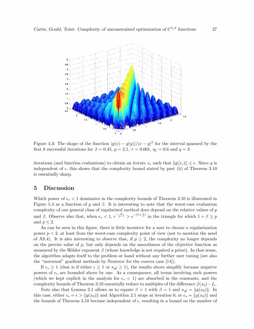
Figure 4.3: The shape of the function |g(x) − g(y)|/|x − y|β for the interval spanned by thefirst 8 successful iterations for β = 0.45, p = 2.1, τ = 0.001, η1 = 0.6 and q = 3

iterations (and function evaluations) to obtain an iterate xε such that ‖g(xε)‖ ≤ ε. Since q isindependent of ε, this shows that the complexity bound stated by part (ii) of Theorem 3.10is essentially sharp.

5 Discussion

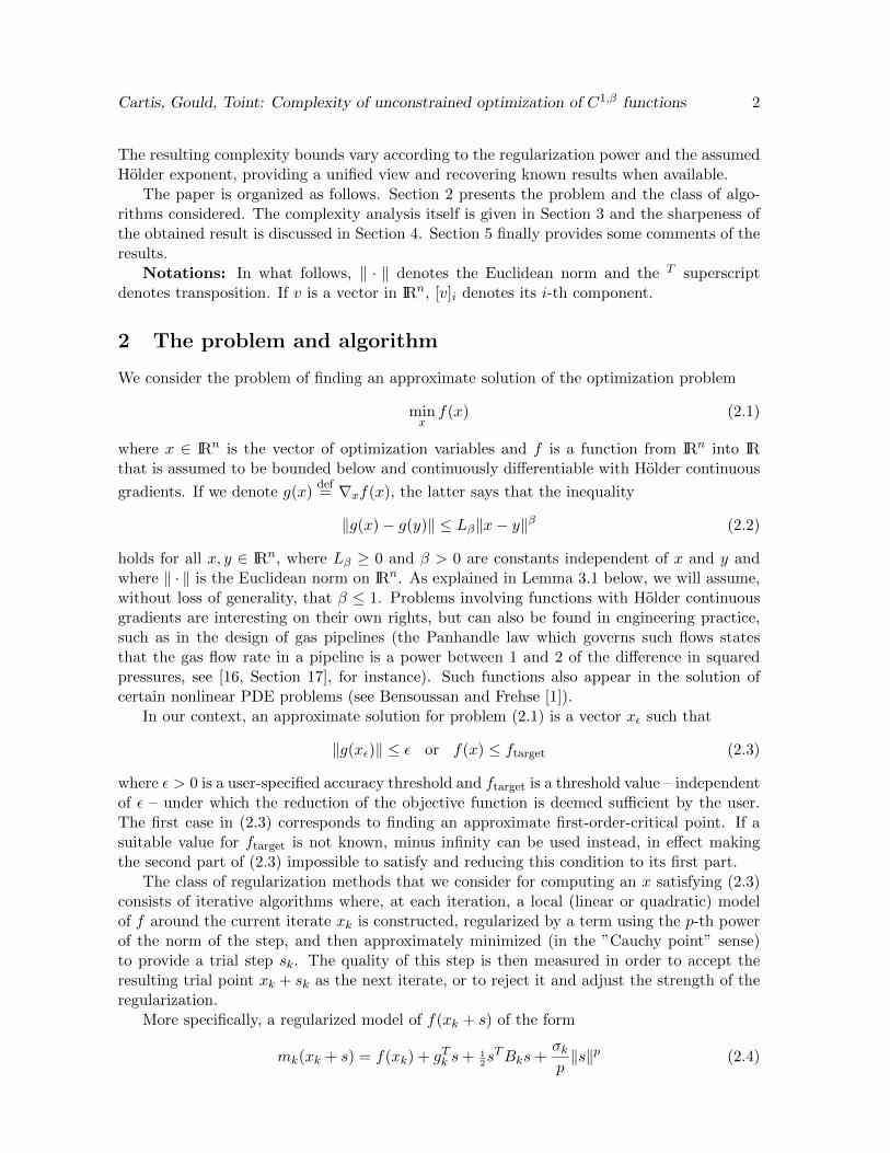
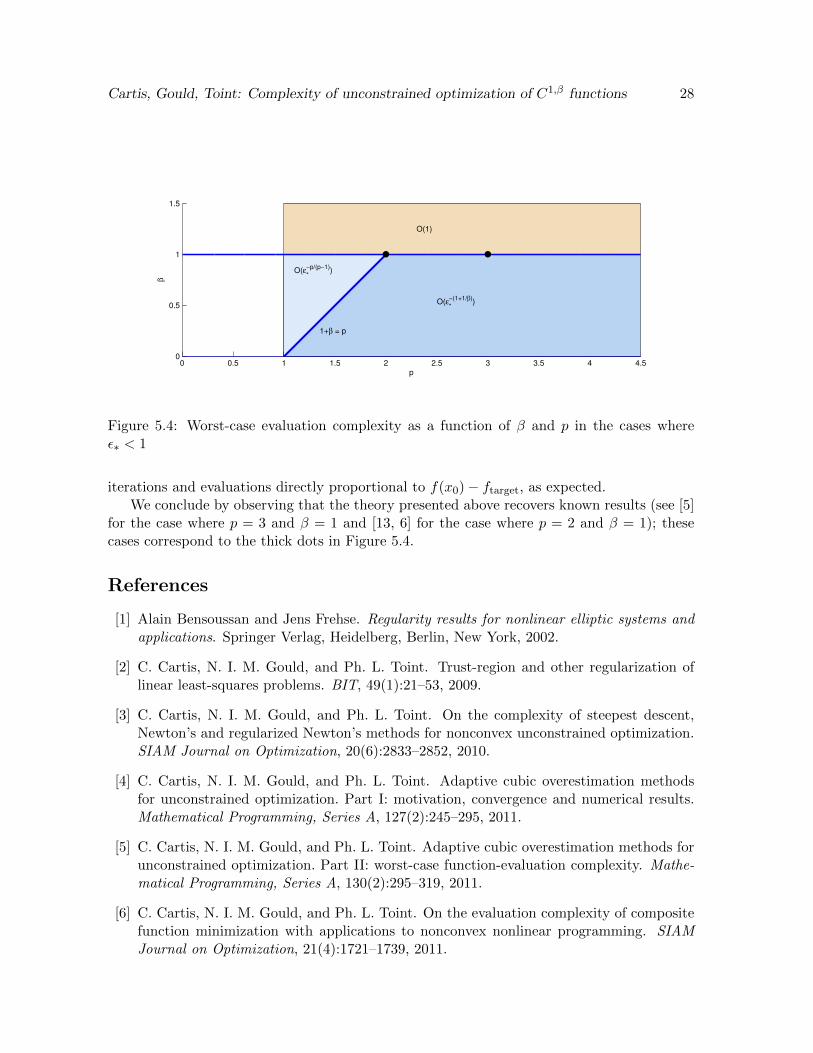
Which power of ε∗ < 1 dominates in the complexity bounds of Theorem 3.10 is illustrated inFigure 5.4 as a function of p and β. It is interesting to note that the worst-case evaluationcomplexity of our general class of regularized method does depend on the relative values of p

and β. Observe also that, when ε∗ < 1, ε− pp−1 > ε

−(1+ 1β)

in the triangle for which 1 + β ≥ pand p ≤ 2.

As can be seen in this figure, there is little incentive for a user to choose a regularizationpower p < 2, at least from the worst-case complexity point of view (not to mention the needof AS.4). It is also interesting to observe that, if p ≥ 2, the complexity no longer dependson the precise value of p, but only depends on the smoothness of the objective function asmeasured by the Holder exponent β (whose knowledge is not required a priori). In that sense,the algorithm adapts itself to the problem at hand without any further user tuning (see alsothe “universal” gradient methods by Nesterov for the convex case [14]).

If ε∗ ≥ 1 (that is if either ε ≥ 1 or κgl ≥ 1), the results above simplify because negativepowers of ε∗ are bounded above by one. As a consequence, all terms involving such powers(which we kept explicit in the analysis for ε∗ < 1) are absorbed in the constants, and thecomplexity bounds of Theorem 3.10 essentially reduce to multiples of the difference f(x0)−f∗.

Note also that Lemma 3.1 allows us to equate β > 1 with β = 1 and κgl = ‖g(x0)‖. Inthis case, either ε∗ = ε > ‖g(x0)‖ and Algorithm 2.1 stops at iteration 0, or ε∗ = ‖g(x0)‖ andthe bounds of Theorem 3.10 become independent of ε, resulting in a bound on the number of


0 0.5 1 1.5 2 2.5 3 3.5 4 4.50

0.5

1

1.5

1+β = p

O(ε*

−(1+1/β))

O(ε*

−p/(p−1))

O(1)

p

β

Figure 5.4: Worst-case evaluation complexity as a function of β and p in the cases whereε∗ < 1

iterations and evaluations directly proportional to f(x0)− ftarget, as expected.We conclude by observing that the theory presented above recovers known results (see [5]

for the case where p = 3 and β = 1 and [13, 6] for the case where p = 2 and β = 1); thesecases correspond to the thick dots in Figure 5.4.

References

[1] Alain Bensoussan and Jens Frehse. Regularity results for nonlinear elliptic systems andapplications. Springer Verlag, Heidelberg, Berlin, New York, 2002.

[2] C. Cartis, N. I. M. Gould, and Ph. L. Toint. Trust-region and other regularization oflinear least-squares problems. BIT, 49(1):21–53, 2009.

[3] C. Cartis, N. I. M. Gould, and Ph. L. Toint. On the complexity of steepest descent,Newton’s and regularized Newton’s methods for nonconvex unconstrained optimization.SIAM Journal on Optimization, 20(6):2833–2852, 2010.

[4] C. Cartis, N. I. M. Gould, and Ph. L. Toint. Adaptive cubic overestimation methodsfor unconstrained optimization. Part I: motivation, convergence and numerical results.Mathematical Programming, Series A, 127(2):245–295, 2011.

[5] C. Cartis, N. I. M. Gould, and Ph. L. Toint. Adaptive cubic overestimation methods forunconstrained optimization. Part II: worst-case function-evaluation complexity. Mathe-matical Programming, Series A, 130(2):295–319, 2011.

[6] C. Cartis, N. I. M. Gould, and Ph. L. Toint. On the evaluation complexity of compositefunction minimization with applications to nonconvex nonlinear programming. SIAMJournal on Optimization, 21(4):1721–1739, 2011.


[7] C. Cartis, N. I. M. Gould, and Ph. L. Toint. On the evaluation complexity of cubicregularization methods for potentially rank-deficient nonlinear least-squares problemsand its relevance to constrained nonlinear optimization. SIAM Journal on Optimization,23(3):15531574, 2013.

[8] N. I. M. Gould, D. P. Robinson, and H. S. Thorne. On solving trust-region and otherregularised subproblems in optimization. Mathematical Programming, Series C, 2(1):21–57, 2010.

[9] G. N. Grapiglia, J. Yuan, and Y. Yuan. Global convergence and worst-case complexity ofa derivative-free trust-region algorithm for composite nonsmooth optimization. Technicalreport, University of Parana, Curitiba, Brasil, 2014.

[10] G. N. Grapiglia, J. Yuan, and Y. Yuan. On the convergence and worst-case complexity oftrust-region and regularization methods for unconstrained optimization. MathematicalProgramming, Series A, (to appear), 2014.

[11] S. Gratton, A. Sartenaer, and Ph. L. Toint. Recursive trust-region methods for multiscalenonlinear optimization. SIAM Journal on Optimization, 19(1):414–444, 2008.

[12] Yu. Nesterov. Introductory Lectures on Convex Optimization. Applied Optimization.Kluwer Academic Publishers, Dordrecht, The Netherlands, 2004.

[13] Yu. Nesterov. Gradient mehods for minimizing composite objective functions. Mathe-matical Programming, Series A, 140(1):125–161, 2013.

[14] Yu. Nesterov. Universal gradient methods for convex optimization problems. Techni-cal Report DP 2013/26140, CORE, Catholic University of Louvain, Louvain-la-Neuve,Belgium, 2013.

[15] Yu. Nesterov and B. T. Polyak. Cubic regularization of Newton method and its globalperformance. Mathematical Programming, Series A, 108(1):177–205, 2006.

[16] Gas Processors and Suppliers Association. Engineering Data Book. Vol. 2. GPSA, Tulsa,USA, 1994.

[17] K. Ueda. A Regularized Newton Method without Line Search for Unconstrained Optimiza-tion. PhD thesis, Department of Applied Mathematics and Physics, Graduate School ofInformatics, Kyoto University, Kyoto, Japan, 2009.

[18] K. Ueda and N. Yamashita. Convergence properties of the regularized Newton methodfor the unconstrained nonconvex optimization. Applied Mathematics & Optimization,62(1):27–46, 2009.

[19] K. Ueda and N. Yamashita. On a global complexity bound of the Levenberg-Marquardtmethod. Journal of Optimization Theory and Applications, 147:443–453, 2010.

[20] L. N. Vicente. Worst case complexity of direct search. EURO Journal on ComputationalOptimization, 1:143–153, 2013.

Documents

Worst-case evaluation complexity of regularization methods ...eprints.maths.ox.ac.uk/1874/1/NA_14_21.pdf · Worst-case evaluation complexity of regularization ... where x2IRn is the