Embed Size (px)
Citation preview
AFRL-RY-WP-TR-2012-0227
THE PRANDTL PLUS SCALING PARAMETERS AND VELOCITY PROFILE SIMILARITY
David Weyburne
Optoelectronic Technology Branch Electromagnetics Technology Division
OCTOBER 2012 Interim Report
Approved for public release; distribution unlimited
AIR FORCE RESEARCH LABORATORY SENSORS DIRECTORATE
WRIGHT-PATTERSON AIR FORCE BASE, OH 45433-7320 AIR FORCE MATERIEL COMMAND
UNITED STATES AIR FORCE
NOTICE AND SIGNATURE PAGE Using Government drawings, specifications, or other data included in this document for any purpose other than Government procurement does not in any way obligate the U.S. Government. The fact that the Government formulated or supplied the drawings, specifications, or other data does not license the holder or any other person or corporation; or convey any rights or permission to manufacture, use, or sell any patented invention that may relate to them. This report was cleared for public release by the USAF 88th Air Base Wing (88 ABW) Public Affairs Office and is available to the general public, including foreign nationals. Copies may be obtained from the Defense Technical Information Center (DTIC) (http://www.dtic.mil). AFRL-RY-WP-TR-2012-0227 HAS BEEN REVIEWED AND IS APPROVED FOR PUBLICATION IN ACCORDANCE WITH ASSIGNED DISTRIBUTION STATEMENT. //SIGNED// //SIGNED// _______________________________________ _______________________________________ DAVID W. WEYBURNE, Work Unit Manager JONAHIRA R. ARNOLD, Chief Optoelectronic Technology Branch Optoelectronic Technology Branch Electromagnetics Technology Division Electromagnetics Technology Division //SIGNED// ______________________________________ WILLIAM E. MOORE, Division Chief Electromagnetics Technology Division Sensors Directorate This report is published in the interest of scientific and technical information exchange, and its publication does not constitute the Government’s approval or disapproval of its ideas or findings. *Disseminated copies will show “//signature//” stamped or typed above the signature blocks.
REPORT DOCUMENTATION PAGE Form Approved OMB No. 0704-0188
The public reporting burden for this collection of information is estimated to average 1 hour per response, including the time for reviewing instructions, searching existing data sources, gathering and maintaining the data needed, and completing and reviewing the collection of information. Send comments regarding this burden estimate or any other aspect of this collection of information, including suggestions for reducing this burden, to Department of Defense, Washington Headquarters Services, Directorate for Information Operations and Reports (0704-0188), 1215 Jefferson Davis Highway, Suite 1204, Arlington, VA 22202-4302. Respondents should be aware that notwithstanding any other provision of law, no person shall be subject to any penalty for failing to comply with a collection of information if it does not display a currently valid OMB control number. PLEASE DO NOT RETURN YOUR FORM TO THE ABOVE ADDRESS.
1. REPORT DATE (DD-MM-YY) 2. REPORT TYPE 3. DATES COVERED (From - To) October 2012 Final 01 October 2011 – 01 May 2012
4. TITLE AND SUBTITLE
THE PRANDTL PLUS SCALING PARAMETERS AND VELOCITY PROFILE SIMILARITY
5a. CONTRACT NUMBER
FA8650-00-M-0000 5b. GRANT NUMBER 5c. PROGRAM ELEMENT NUMBER
62204F 6. AUTHOR(S)
David Weyburne 5d. PROJECT NUMBER
4916 5e. TASK NUMBER
HC 5f. WORK UNIT NUMBER
4916HC10/Y0AX 7. PERFORMING ORGANIZATION NAME(S) AND ADDRESS(ES) 8. PERFORMING ORGANIZATION
REPORT NUMBER
AFRL-RY-WP-TR-2012-0227 Optoelectronic Technology Branch Electromagnetics Technology Division Air Force Research Laboratory, Sensors Directorate Wright-Patterson Air Force Base, OH 45433-7320 Air Force Materiel Command, United States Air Force
9. SPONSORING/MONITORING AGENCY NAME(S) AND ADDRESS(ES) Air Force Research Laboratory Sensors Directorate Wright-Patterson Air Force Base, OH 45433-7320 Air Force Materiel Command United States Air Force
10. SPONSORING/MONITORING AGENCY ACRONYM(S)
AFRL/RYHC 11. SPONSORING/MONITORING AGENCY REPORT NUMBER(S)
AFRL-RY-WP-TR-2012-0227 12. DISTRIBUTION/AVAILABILITY STATEMENT
Approved for public release; distribution unlimited. 13. SUPPLEMENTARY NOTES
This is a work of the U.S. Government and is not subject to copyright protection in the United States. PAO Case Number 88ABW-2012-4071, Clearance Date 19 July 2012. Report contains color.
14. ABSTRACT Numerous experimental results have demonstrated similar behavior of the velocity profile in the near-wall region of the turbulent boundary layer using Prandtl’s “Plus” scaling variables. However, the implications for similarity behavior of the near-wall turbulent boundary velocity profiles using Prandtl’s Plus scaling variables have not been carefully explored. In the following report, we apply the momentum balance type approach to study velocity profile similarity using Prandtl’s Plus scaling variables. It is shown that the Plus scaling variables do in fact satisfy the requirements for similarity based on this approach so long as the friction velocity is proportional to 1/(x-x0) where x is the distance along the wall in the flow direction and x0 is a constant. Experimental results are examined and found to confirm that certain datasets we tested do in fact have the friction velocity values behaving as 1/(x-x0). We show the Plus scaling variables satisfy all of the conditions for similarity using the momentum balance type approach for these datasets. However, the same velocity profile dataset plots also confirm that Prandtl’s Plus scaling variables do not show whole profile similarity. Hence, we conclude that the scaling variables discovered by the momentum balance type approach as presently constituted are a necessary but not sufficient condition for velocity profile similarity..
15. SUBJECT TERMS Fluid Boundary Layer, Prandtl Plus Scaling, Boundary Layer Flow, Velocity Profile Similarity, Momentum Balance Equation
16. SECURITY CLASSIFICATION OF: 17. LIMITATION OF ABSTRACT:
SAR
18. NUMBER OF PAGES
28
19a. NAME OF RESPONSIBLE PERSON (Monitor)
a. REPORT Unclassified
b. ABSTRACT Unclassified
c. THIS PAGE Unclassified
Jonahira Arnold 19b. TELEPHONE NUMBER (Include Area Code)
N/A Standard Form 298 (Rev. 8-98)
Prescribed by ANSI Std. Z39-18
i Approved for public release; distribution unlimited
TABLE OF CONTENTS
Section Page
List of Figures . . . . . . . . . . . . . . . . . . . . . . . . . . . . . . . . . . . . . . . . . . . . . . . . . . . . . . . . . . . . . . . . . . . . . . . . ii Acknowledgments . . . . . . . . . . . . . . . . . . . . . . . . . . . . . . . . . . . . . . . . . . . . . . . . . . . . . . . . . . . . . . . . . . . . iii Summary . . . . . . . . . . . . . . . . . . . . . . . . . . . . . . . . . . . . . . . . . . . . . . . . . . . . . . . . . . . . . . . . . . . . . . . . . . . . . . 1 1. Introduction . . . . . . . . . . . . . . . . . . . . . . . . . . . . . . . . . . . . . . . . . . . . . . . . . . . . . . . . . . . . . . . . . . . . . . . . 2 2. Similarity Equations . . . . . . . . . . . . . . . . . . . . . . . . . . . . . . . . . . . . . . . . . . . . . . . . . . . . . . . . . . . . . 3 2.1 Near-Wall Flow Similarity . . . . . . . . . . . . . . . . . . . . . . . . . . . . . . . . . . . . . . . . . . . . . . . . . . . 5 2.2 Outer Region Flow Similarity . . . . . . . . . . . . . . . . . . . . . . . . . . . . . . . . . . . . . . . . . . . . . . . . . 5 3. Prandtl Plus Scaling Similarity . . . . . . . . . . . . . . . . . . . . . . . . . . . . . . . . . . . . . . . . . . . . . . . . . . . . . . 6 4. Experimental Verification . . . . . . . . . . . . . . . . . . . . . . . . . . . . . . . . . . . . . . . . . . . . . . . . . . . . . . . . . . . . 7 5. Discussion . . . . . . . . . . . . . . . . . . . . . . . . . . . . . . . . . . . . . . . . . . . . . . . . . . . . . . . . . . . . . . . . . . 14 6. Conclusion . . . . . . . . . . . . . . . . . . . . . . . . . . . . . . . . . . . . . . . . . . . . . . . . . . . . . . . . . . . . . 15 References . . . . . . . . . . . . . . . . . . . . . . . . . . . . . . . . . . . . . . . . . . . . . . . . . . . . . . . . . . . . . . . . 16 Appendix 1 . . . . . . . . . . . . . . . . . . . . . . . . . . . . . . . . . . . . . . . . . . . . . . . . . . . . . . . . . . . . . . . . 18
ii Approved for public release; distribution unlimited
LIST OF FIGURES
Figure 1a: Eight Causer [4] scaled velocity profiles (IDENT 2200) plotted using Plus units. . . . 8 Figure 1b: The Causer [4] friction velocity values (+) along with the a/(x-x0) fitted line. . . . . . . 8 Figure 1c: The Causer [4] velocity ratio values (+) along with the average value line. . . . . . . . . 8 Figure 2a: Six Herring and Norbury [11] scaled velocity profiles (IDENT 2700) plotted using Plus units. . . . . . . . . . . . . . . . . . . . . . . . . . . . . . . . . . . . . . . . . . . . . . . . . . . . 9 Figure 2b: The Herring and Norbury [11] friction velocity values (+) along with the a/(x-x0) fitted line. . . . . . . . . . . . . . . . . . . . . . . . . . . . . . . . . . . . . . . . . . . . . . . . . . . . . . . . . . . . . . . . . . . . . . . . . 9 Figure 2c: The Herring and Norbury [11] velocity ratios (+) along with the average value line. . . . . . . . . . . . . . . . . . . . . . . . . . . . . . . . . . . . . . . . . . . . . . . . . . . . . . . . . . . . . . . . . . . . . . . . . . . . . . 9 Figure 3a: Seven Skåre and Krogstad [12] scaled velocity profiles plotted using Plus units. . . 10 Figure 3b: The Skåre and Krogstad [12] friction velocity values (+) along with the a/(x-x0) fitted line. . . . . . . . . . . . . . . . . . . . . . . . . . . . . . . . . . . . . . . . . . . . . . . . . . . . . . . . . . . . . . . . . . . . . . . . 10 Figure 3c: The Skåre and Krogstad [12] velocity ratio values (+) along with the average value line. . . . . . . . . . . . . . . . . . . . . . . . . . . . . . . . . . . . . . . . . . . . . . . . . . . . . . . . . . . . . . . . . . . . . . . . 10 Figure 4a: Four Bradshaw and Ferriss [13] scaled velocity profiles (IDENT 2600) plotted using Plus units. . . . . . . . . . . . . . . . . . . . . . . . . . . . . . . . . . . . . . . . . . . . . . . . . . . . . . . . . . . . . . . . . . . 11 Figure 4b: The Bradshaw and Ferriss [13] friction velocity values (+) along with the a/(x-x0) fitted line. . . . . . . . . . . . . . . . . . . . . . . . . . . . . . . . . . . . . . . . . . . . . . . . . . . . . . . . . . . . . 11 Figure 4c: The Bradshaw and Ferriss [13] velocity ratio values (+) along with the average value line. . . . . . . . . . . . . . . . . . . . . . . . . . . . . . . . . . . . . . . . . . . . . . . . . . . . . . . . . . . . . . . . . . . . . . . 11 Figure 5a: Twelve Jones, Marusic, and Perry [14] scaled velocity profiles (from x = 2400 to 3620 mm, K= 2.7 × 10⁻⁷) plotted using Plus units. . . . . . . . . . . . . . . . . . . . . . . . . . . . . . . . . . . . 12 Figure 5b: Jones, Marusic, and Perry [14] friction velocity values (+) along with the a/(x-x0) fitted line. . . . . . . . . . . . . . . . . . . . . . . . . . . . . . . . . . . . . . . . . . . . . . . . . . . . . . . . . . . . . . . . 12 Figure 5c: Jones, Marusic, and Perry [14] velocity ratio values (+) along with the average value line. . . . . . . . . . . . . . . . . . . . . . . . . . . . . . . . . . . . . . . . . . . . . . . . . . . . . . . . . . . . . . . . . . . . . . . 12 Figure 6a: Ten Smith and Smits [15] scaled velocity profiles plotted using Plus units. . . . . . . 13 Figure 6b: The Smith and Smits [15] friction velocity values (+) along with the a/(x-x0) fitted line. . . . . . . . . . . . . . . . . . . . . . . . . . . . . . . . . . . . . . . . . . . . . . . . . . . . . . . . . . . . . . . . . . . . . . . 13 Figure 7a: Fifteen Wieghardt and Tillmann [15] scaled velocity profiles (IDENT 1400, from 1.087 to 4.987 m) plotted using Plus units. . . . . . . . . . . . . . . . . . . . . . . . . . . . . . . . . . . . . . . . . 13 Figure 7b. The Wieghardt and Tillmann [15] friction velocity values (+) along with the a/(x-x0) fitted line. . . . . . . . . . . . . . . . . . . . . . . . . . . . . . . . . . . . . . . . . . . . . . . . . . . . . . . . . . . . . . . . . 13
iii Approved for public release; distribution unlimited
ACKNOWLEDGEMENT
The author would like to thank the following groups and individuals for making their experimental datasets available for inclusion in this manuscript: Francis Clauser; H. Herring, and J. Norbury; Per Egil Skåre and Per-Åge Krogstad; Peter Bradshaw and D. Ferriss; Malcolm Jones, Ivan Marusic, and Anthony Perry; Randall Smith and Alexander Smits; and Karl Wieghardt and W. Tillmann.
1 Approved for public release; distribution unlimited
SUMMARY
Numerous experimental results have demonstrated similar behavior of the velocity profile in the near-wall region of the turbulent boundary layer using Prandtl’s “Plus” scaling variables. However, the implications for similarity behavior of the near-wall turbulent boundary velocity profiles using Prandtl’s Plus scaling variables have not been carefully explored. In the following report, we apply the momentum balance type approach to study velocity profile similarity using Prandtl’s Plus scaling variables for the wall-bounded turbulent boundary layer. It is shown that the Plus scaling variables will in fact satisfy the requirements for similarity based on this approach so long as the friction velocity values in the flow direction are proportional to 01/( )x x− where x is the distance along the wall in the flow direction and 0x is a constant. Experimental results are examined and found to confirm that certain datasets we tested do in fact have the friction velocity values behaving as 01/( )x x− . For these datasets, we show the Plus scaling variables satisfy all of the conditions for similarity using the momentum balance type approach. However, the same velocity profile dataset plots also confirm that Prandtl’s Plus scaling variables do not show whole profile similarity in general. Hence, we conclude that the scaling variables discovered by the momentum balance type approach as presently constituted are a necessary but not sufficient condition for velocity profile similarity.
2 Approved for public release; distribution unlimited
1. INTRODUCTION Beginning with the pioneering work of Reynolds [1], there has been a concerted effort to find coordinate scaling parameters that make the scaled velocity profiles and shear-stress profiles taken at different stations along the wall in the flow direction to appear to be similar. For turbulent boundary layers, the early search for similarity was mostly unsuccessful. This led to the practice of trying to find similarity in subregions of the whole profile. Perhaps the most successful case of partial similarity was developed by von Kármán [2] and Prandtl [3] and is known as the Logarithmic Law or “Log Law.” The Log Law states that in a region adjacent to the wall of the turbulent boundary layer the average velocity in the streamwise x-direction of a wall-bounded turbulent flow is given by
( ), 1 ln ,u x y yu
Bu
τ
τ κ ν ≅ +
where y is the height perpendicular to the solid surface , ν is kinematic viscosity, κ and B are constants, and uτ is the Prandtl velocity scaling parameter, the so-called
friction velocity. Experimental plots of the wall-bounded turbulent boundary layer velocity profiles taken at various stations along the wall using uτ as the velocity scaling parameter and /uτν as
the length scaling parameter (the so-called “Plus” scaling factors) have consistently demonstrated similarity-like behavior in the near-wall region of the profile. There has been much debate as to whether this is due to the fact that the Log Law or, as some believe, a Power Law that is universally applicable for all wall-bounded turbulent flows. In any case, one area that has not been explored is the similarity implications using the friction velocity as the key scaling variable. For example, the question of whether the Prandtl’s Plus scaling variables even satisfy the conditions for similarity has not been studied. The standard approach for studying similarity is to use the dimensionless momentum balance equation. The search for similarity scaling behavior for the turbulent boundary layer using this approach began with the experimental and theoretical work of Clauser [4]. Using the friction velocity uτ as the velocity scaling variable and the displacement thickness 1δ as the length scaling variable, Clauser predicted that
equilibrium (similar) boundary layers are only obtained for the nonzero pressure gradient case when the quantity
12
edpu dxττ
δβ
ρ= −
is a constant. In this equation ρ is the density and ep is the pressure at the boundary layer edge. Rotta [5] and Townsend [6] subsequently developed some additional theoretical considerations for turbulent boundary layer similarity using this approach.
(1)
(2)
3 Approved for public release; distribution unlimited
More recently, Castillo and George [7] used this approach and found that similarity will exist only when the parameter
s
s
du dxu d dxδ
δΛ = −
is a constant. In this equation δ is an as yet unspecified thickness scaling variable and )(xus is an as yet unspecified scaling velocity. Following a similar scheme of keeping
the thickness scaling variable and the velocity scaling variables as unspecified, Weyburne [8] added the dimensionless Reynolds stress transport equation to obtain additional restrictions with the result that it was shown that in the outer region of the turbulent boundary layer δ must be a linear function of the type 1 0( )a x xδ = − and su
must be s eu u∝ and a power law function of the type 2 0( )meu a x x= − , such that 1a , 2a ,
m, and 0x are constants. What is relevant here is that in none of these previous momentum balance type approaches have explicitly tested using uτ as the velocity scaling parameter and /uτν as
the length scaling parameter to find out whether they satisfy the conditions for similarity of the velocity profiles of a turbulent boundary layer. In what follows, we take on this task. Using the momentum balance equation type analysis, we first confirm theoretically that the unknown thickness scaling variable δ and the unknown scaling velocity )(xus must behave in a manner consistent with the sink flow/wedge flow solution. It is shown that the Plus scaling variables will in fact satisfy this requirement for similarity based on the momentum balance equation approach so long as the friction velocity values in the flow direction are proportional to 01/( )x x− where x is the distance along the wall in the flow direction and 0x is a constant. Experimental results are examined and found to confirm that certain datasets we tested do in fact satisfy all the conditions of whole profile similarity based on the momentum balance type approach requirements. However, the same plots also confirm that Prandtl’s Plus scaling variables based plots do not show velocity profile similarity over the whole boundary layer region. Hence, we conclude that the scaling variables discovered by the momentum balance type approach are a necessary but not sufficient condition for velocity profile similarity.
2. SIMILARITY EQUATIONS
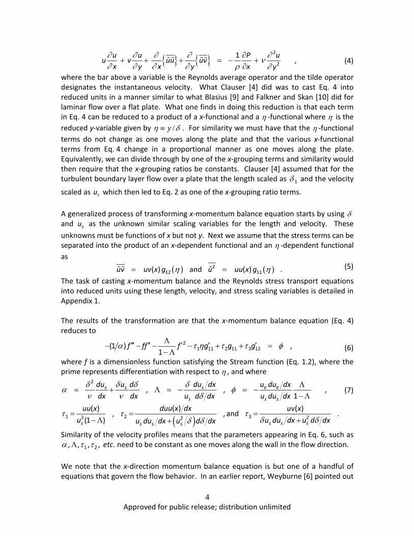
The theoretical guidance for discovering similarity scaling laws for the turbulent boundary layer started with Clauser [4] who looked at the implications of similarity using the x-momentum balance equation. For a 2-D incompressible turbulent boundary layer that is steady state on the mean, the Reynolds-averaged stream-direction component (x-direction) of the momentum balance for flow along a plate is given by
(3)
4 Approved for public release; distribution unlimited
{ } { }2
21 ,u u P uu v uu uv
x y x y x y∂ ∂ ∂ ∂ ∂ν∂ ∂ ∂ ∂ ρ ∂
∂+ + + = − +
∂
where the bar above a variable is the Reynolds average operator and the tilde operator designates the instantaneous velocity. What Clauser [4] did was to cast Eq. 4 into reduced units in a manner similar to what Blasius [9] and Falkner and Skan [10] did for laminar flow over a flat plate. What one finds in doing this reduction is that each term in Eq. 4 can be reduced to a product of a x-functional and a η -functional where η is the reduced y-variable given by /η δ≡ y . For similarity we must have that the η -functional terms do not change as one moves along the plate and that the various x-functional terms from Eq. 4 change in a proportional manner as one moves along the plate. Equivalently, we can divide through by one of the x-grouping terms and similarity would then require that the x-grouping ratios be constants. Clauser [4] assumed that for the turbulent boundary layer flow over a plate that the length scaled as 1δ and the velocity
scaled as uτ which then led to Eq. 2 as one of the x-grouping ratio terms. A generalized process of transforming x-momentum balance equation starts by using δ and su as the unknown similar scaling variables for the length and velocity. These unknowns must be functions of x but not y. Next we assume that the stress terms can be separated into the product of an x-dependent functional and an η -dependent functional as
( ) ( )212 11( ) and ( ) .uv uv x g u uu x gη η= =
The task of casting x-momentum balance and the Reynolds stress transport equations into reduced units using these length, velocity, and stress scaling variables is detailed in Appendix 1. The results of the transformation are that the x-momentum balance equation (Eq. 4) reduces to
21 11 2 11 3 12(1 ) ,
1f ff f g g gα τ η τ τ φΛ′′′ ′′ ′ ′ ′− − − − + + =
−Λ
where f is a dimensionless function satisfying the Stream function (Eq. 1.2), where the prime represents differentiation with respect to η , and where
( )
2
1 2 32 22
, , ,1
( )( ) ( ), , and .(1 )
s e es s
s s s
s s s ss s s
du dx u du dxdu u ddx dx u d dx u du dx
duu x dxuu x uv xu u du dx u d dxu du dx u d dx
δδ δ δα φν ν δ
τ τ τδ δδ δ
Λ= + Λ = − = −
−Λ
= = =−Λ ++
Similarity of the velocity profiles means that the parameters appearing in Eq. 6, such as1 2, , , ,α τ τΛ etc. need to be constant as one moves along the wall in the flow direction.
We note that the x-direction momentum balance equation is but one of a handful of equations that govern the flow behavior. In an earlier report, Weyburne [6] pointed out
(4)
(5)
(6)
(7)
5 Approved for public release; distribution unlimited
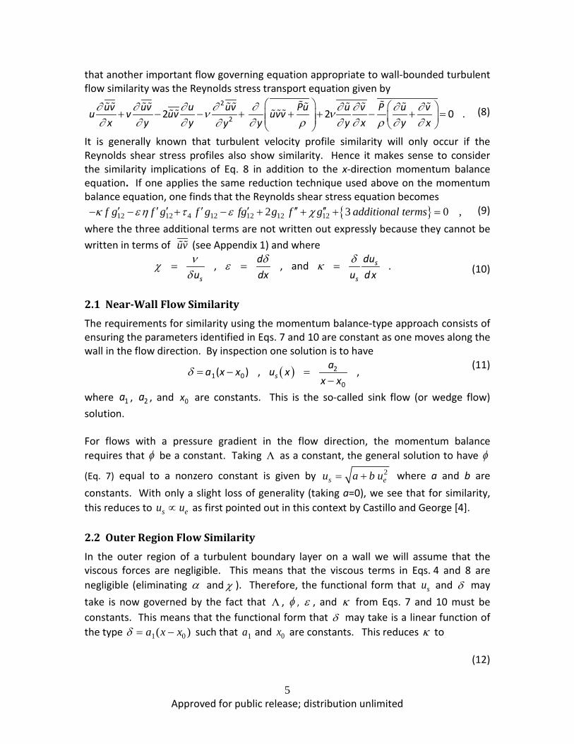
that another important flow governing equation appropriate to wall-bounded turbulent flow similarity was the Reynolds stress transport equation given by
2
22 2 0 .uv uv u uv Pu u v P u vu v uv uvvx y y y y x y xy
∂ ∂ ∂ ∂ ∂ ∂ ∂ ∂ ∂ν ν∂ ∂ ∂ ∂ ρ ∂ ∂ ρ ∂ ∂∂
+ − − + + + − + =
It is generally known that turbulent velocity profile similarity will only occur if the Reynolds shear stress profiles also show similarity. Hence it makes sense to consider the similarity implications of Eq. 8 in addition to the x-direction momentum balance equation. If one applies the same reduction technique used above on the momentum balance equation, one finds that the Reynolds shear stress equation becomes
{ }12 12 4 12 12 12 122 3 0 ,κ εη τ ε χ′ ′ ′ ′ ′ ′′ ′′− − + − + + + =f g f g f g fg g f g additional terms
where the three additional terms are not written out expressly because they cannot be written in terms of uv (see Appendix 1) and where
, , and .s
s s
dudu dx u d xν δ δχ ε κδ
= = =
2.1 Near-Wall Flow Similarity
The requirements for similarity using the momentum balance-type approach consists of ensuring the parameters identified in Eqs. 7 and 10 are constant as one moves along the wall in the flow direction. By inspection one solution is to have
( ) 21 0
0( ) , ,s
aa x x u xx x
δ = − =−
where 1a , 2a , and 0x are constants. This is the so-called sink flow (or wedge flow) solution. For flows with a pressure gradient in the flow direction, the momentum balance requires that φ be a constant. Taking Λ as a constant, the general solution to have φ
(Eq. 7) equal to a nonzero constant is given by 2s eu a b u= + where a and b are
constants. With only a slight loss of generality (taking a=0), we see that for similarity, this reduces to s eu u∝ as first pointed out in this context by Castillo and George [4]. 2.2 Outer Region Flow Similarity
In the outer region of a turbulent boundary layer on a wall we will assume that the viscous forces are negligible. This means that the viscous terms in Eqs. 4 and 8 are negligible (eliminating α and χ ). Therefore, the functional form that su and δ may take is now governed by the fact that Λ , φ , ε , and κ from Eqs. 7 and 10 must be constants. This means that the functional form that δ may take is a linear function of the type 1 0( )a x xδ = − such that 1a and 0x are constants. This reduces κ to
(8)
(9)
(10)
(11)
(12)
6 Approved for public release; distribution unlimited
1 0( ),s
s
a x x duu d x
κ−
=
which has the general solution of ( ) ( )2 0su x a x x κ= −
where 2a is a constant. For flows with a pressure gradient in the flow direction, the momentum balance requires that φ be a constant. The general solution to have φ (Eq. 7) equal to a nonzero
constant is given by 2s eu a b u= + where a and b are constants. With only a slight loss
of generality (taking a=0), we see that for similarity, this reduces to s eu u∝ as first pointed out in this context by Castillo and George [4].
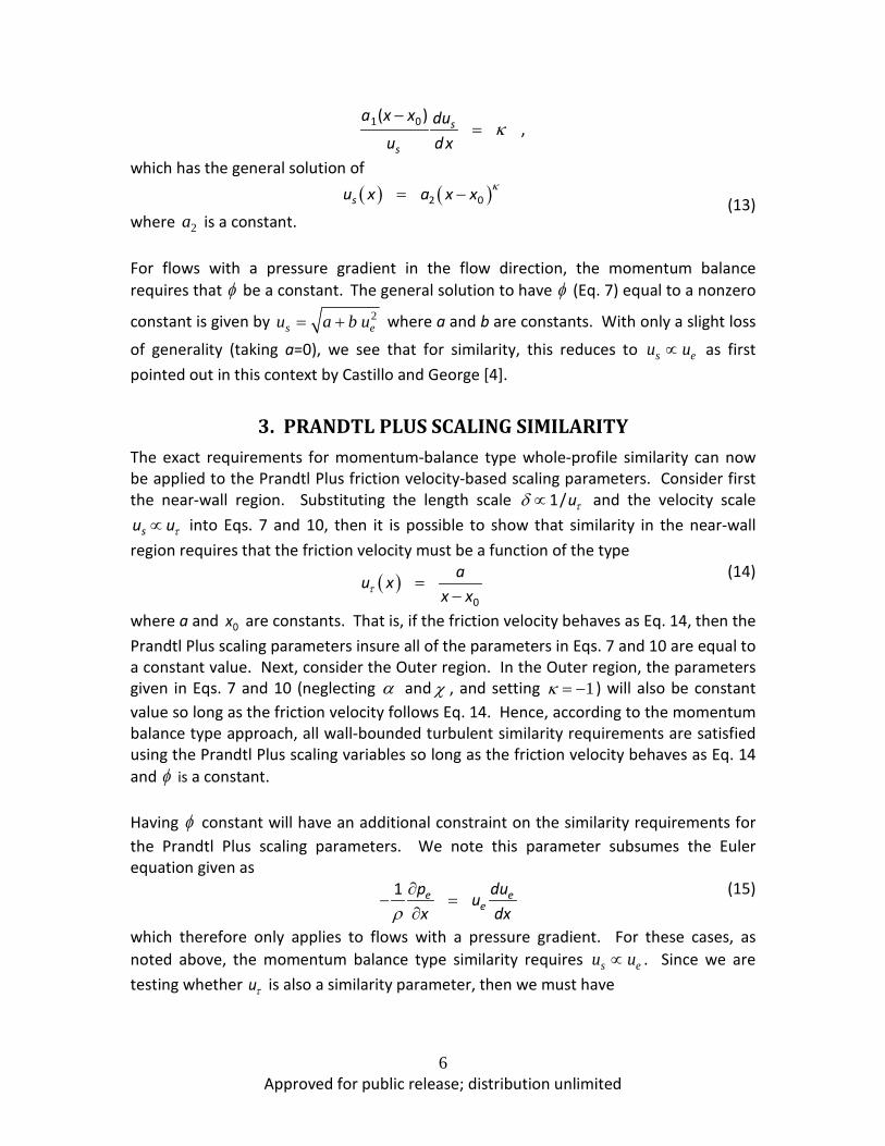
3. PRANDTL PLUS SCALING SIMILARITY The exact requirements for momentum-balance type whole-profile similarity can now be applied to the Prandtl Plus friction velocity-based scaling parameters. Consider first the near-wall region. Substituting the length scale 1/uτδ ∝ and the velocity scale
su uτ∝ into Eqs. 7 and 10, then it is possible to show that similarity in the near-wall region requires that the friction velocity must be a function of the type
( )0
au xx xτ =−
where a and 0x are constants. That is, if the friction velocity behaves as Eq. 14, then the Prandtl Plus scaling parameters insure all of the parameters in Eqs. 7 and 10 are equal to a constant value. Next, consider the Outer region. In the Outer region, the parameters given in Eqs. 7 and 10 (neglecting α and χ , and setting 1κ = − ) will also be constant value so long as the friction velocity follows Eq. 14. Hence, according to the momentum balance type approach, all wall-bounded turbulent similarity requirements are satisfied using the Prandtl Plus scaling variables so long as the friction velocity behaves as Eq. 14 and φ is a constant. Having φ constant will have an additional constraint on the similarity requirements for the Prandtl Plus scaling parameters. We note this parameter subsumes the Euler equation given as
1 e ee
p duu
x dxρ∂
− =∂
which therefore only applies to flows with a pressure gradient. For these cases, as noted above, the momentum balance type similarity requires s eu u∝ . Since we are testing whether uτ is also a similarity parameter, then we must have
(13)
(14)
(15)
7 Approved for public release; distribution unlimited
constant,euuτ
=
the so-called Rotta constraint.
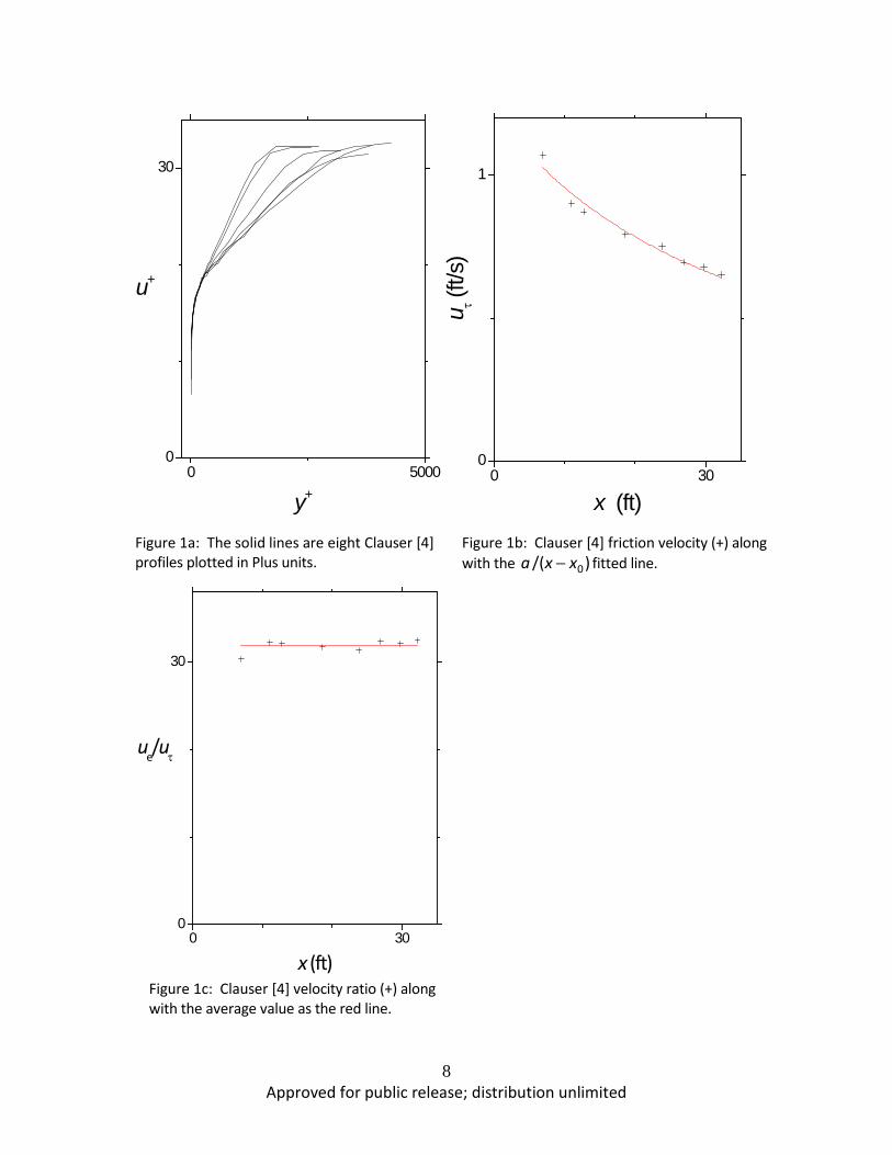
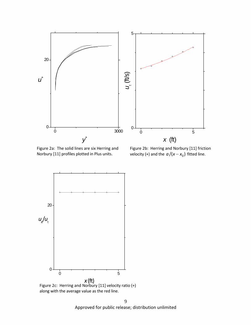
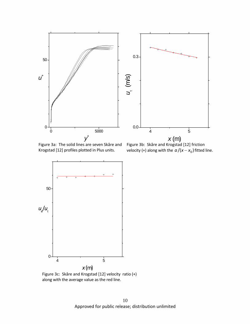
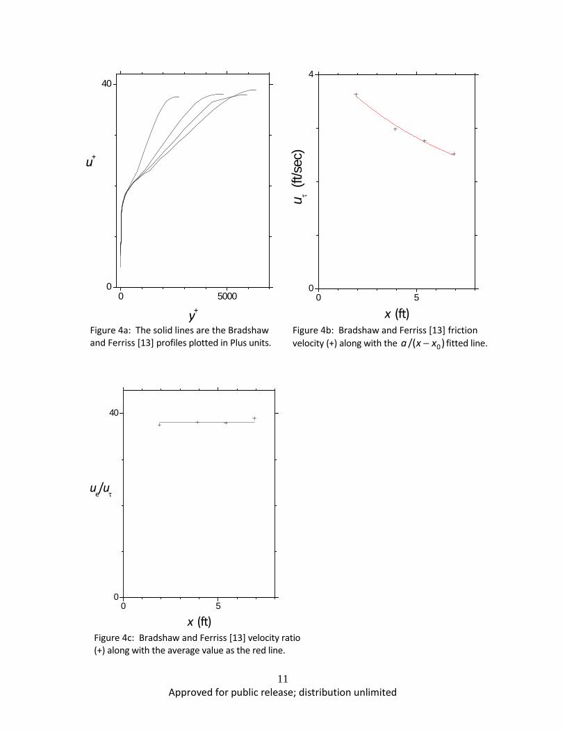
4. EXPERIMENTAL VERIFICATION We are now in a position to answer the question as to whether the Prandtl Plus friction velocity-based scaling parameters satisfy the momentum-balance type whole-profile similarity requirements. A number of datasets from the literature were selected based on satisfying Eq. 16. In Figs. 1a-7a we plot some sets of velocity profiles in which the plot axes are put in reduced units using the Prandtl Plus friction velocity-based scaling parameters. In these figures the wall is located at 0y+ = . In all cases there is a region near the wall for which all of the profiles overlap, i.e. they display near-wall similarity behavior. The question we want to answer is whether these same datasets also satisfy the condition for whole-profile similarity, that is does the friction velocity values fit to Eq. 14 and is Eq. 16 satisfied. First, consider the friction velocity fits. In Figs. 1b-7b we plot the experimental friction velocity as points (+) versus the station location for each corresponding dataset. The red line in each plot is the least squares fit to the points using Eq. 14. In general, the fits are good indicating that Prandtl Plus scaling factors do in fact satisfy the condition for constant parameter ratios (Eqs. 7 and 10). For the flows considered in Figs. 1-5, which do have a pressure gradient present in the flow direction, we must also have Eq. 16 hold if uτ is to be a similarity parameter. This
condition is checked in Figs. 1c-5c which plots this velocity ratio along with average velocity ratio value as the red line. As is evident from the plots, this constraint does in fact hold for these datasets (recall that in fact these datasets were selected based on this criterion). It is necessary to note that datasets presented in Figs. 6 and 7 are for flat plate flows for which dp/dx=0, and therefore the φ parameter constraint is not applicable. The experimental results presented above indicate that all of these datasets satisfy the conditions for similarity using the momentum balance type approach when using uτ as
the velocity scaling parameter and 1/uτ as the length scaling parameter. However, it
also apparent from Figs. 1a-7a that these datasets do not in general display velocity profile similarity over the whole profile.
(16)
8 Approved for public release; distribution unlimited
0 50000
30
u+
y+0 30
0
1
u τ (f
t/s)
x (ft)
0 300
30
ue/uτ
x (ft)
Figure 1a: The solid lines are eight Clauser [4] profiles plotted in Plus units.
Figure 1b: Clauser [4] friction velocity (+) along with the 0/( )a x x− fitted line.
Figure 1c: Clauser [4] velocity ratio (+) along with the average value as the red line.
9 Approved for public release; distribution unlimited
0 30000
20
u+
y+0 5
0
5
u τ (f
t/s)
x (ft)
0 50
20
ue/uτ
x (ft)
Figure 2a: The solid lines are six Herring and Norbury [11] profiles plotted in Plus units.
Figure 2b: Herring and Norbury [11] friction velocity (+) and the 0/( )a x x− fitted line.
Figure 2c: Herring and Norbury [11] velocity ratio (+) along with the average value as the red line.
10 Approved for public release; distribution unlimited
0 50000
50
u+
y+4 5
0.0
0.3
u τ (
m/s
)
x (m)
4 50
50
ue/uτ
x (m)
Figure 3a: The solid lines are seven Skåre and Krogstad [12] profiles plotted in Plus units.
Figure 3b: Skåre and Krogstad [12] friction velocity (+) along with the 0/( )a x x− fitted line.
Figure 3c: Skåre and Krogstad [12] velocity ratio (+) along with the average value as the red line.
11 Approved for public release; distribution unlimited
0 50000
40
u+
y+0 5
0
4
u τ (
ft/se
c)x (ft)
0 50
40
ue/uτ
x (ft)
Figure 4a: The solid lines are the Bradshaw and Ferriss [13] profiles plotted in Plus units.
Figure 4b: Bradshaw and Ferriss [13] friction velocity (+) along with the 0/( )a x x− fitted line.
Figure 4c: Bradshaw and Ferriss [13] velocity ratio (+) along with the average value as the red line.
12 Approved for public release; distribution unlimited
0 30000
20
u+
y+0 3000
0
1
u τ (m
/s)
x (mm)
2000 30000
20
ue/uτ
x (mm)
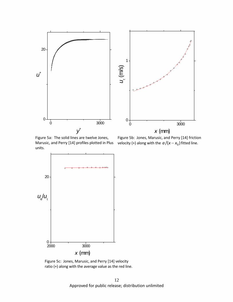
Figure 5a: The solid lines are twelve Jones, Marusic, and Perry [14] profiles plotted in Plus units.
Figure 5b: Jones, Marusic, and Perry [14] friction velocity (+) along with the 0/( )a x x− fitted line.
Figure 5c: Jones, Marusic, and Perry [14] velocity ratio (+) along with the average value as the red line.
13 Approved for public release; distribution unlimited
0 50000
20
u+
y+1 2 3 4
0
1
uτ
x (m)
0 50000
30
u+
y+0 5
0
1
u τ (
m/s
)
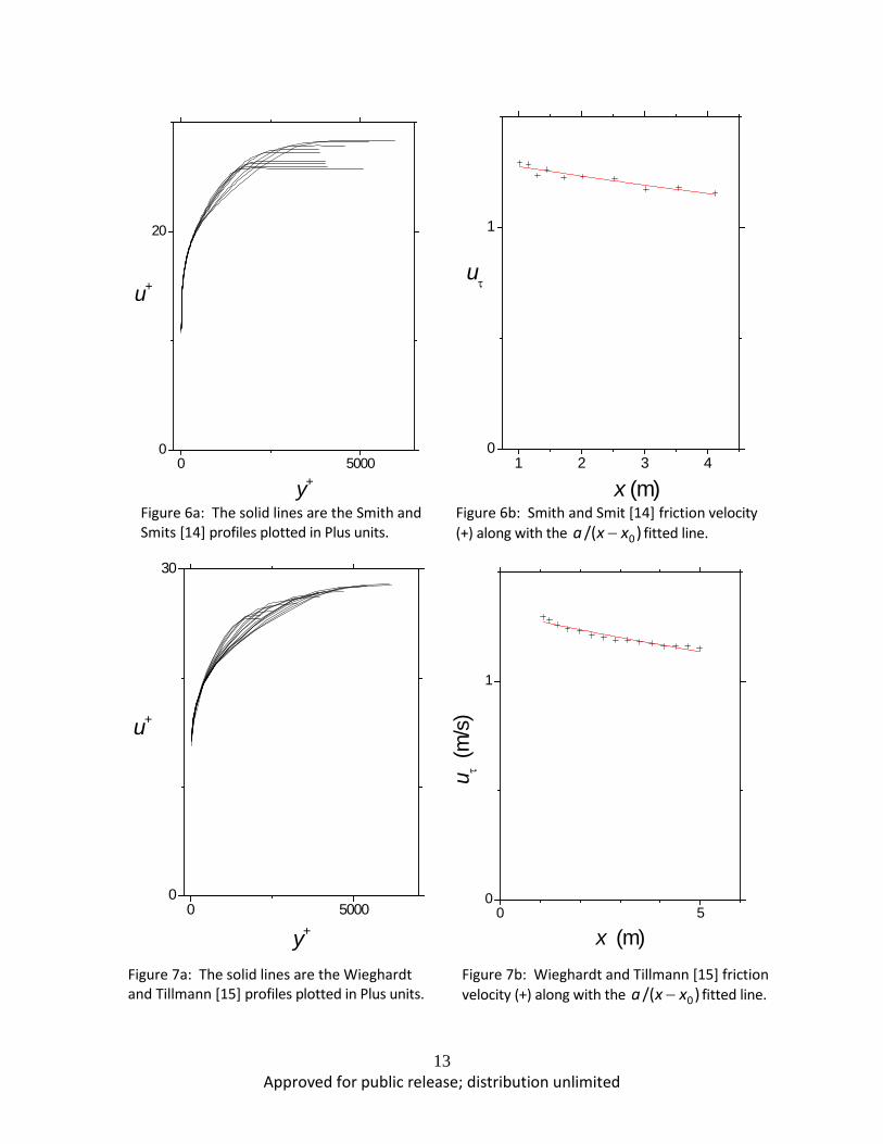
x (m)Figure 7a: The solid lines are the Wieghardt and Tillmann [15] profiles plotted in Plus units.
Figure 7b: Wieghardt and Tillmann [15] friction velocity (+) along with the 0/( )a x x− fitted line.
Figure 6a: The solid lines are the Smith and Smits [14] profiles plotted in Plus units.
Figure 6b: Smith and Smit [14] friction velocity (+) along with the 0/( )a x x− fitted line.
14 Approved for public release; distribution unlimited
5. DISCUSSION The implications of the above results should be viewed in the context of two observations which stand out: 1) in spite of satisfying all of the requirements, the set of profiles given in Figs. 1a-7a clearly demonstrate that the Prandtl Plus scaling parameters do NOT, in general, result in similarity flow behavior (except at the near-wall), and 2) while the length scale 1/uτδ ∝ and the velocity scale su uτ∝ have the correct x-behavior (Eq. 14), it is necessary to point out that only two of the geometries considered in Figs. 1-7 conform to the traditional sink flow/wedge flow geometry. Consider the first observation, that is, the Prandtl Plus scaling parameters do NOT in general result in similarity flow behavior in spite of satisfying all of the conditions for similarity using the momentum balance type approach. First of all we must point out that the datasets chosen above were not picked at random. They were picked because the experiments in question were intentionally (or unintentionally) set up specifically to obtain similar profiles. In fact only a handful of wall-bounded turbulent boundary layer datasets fall into this category. In any case, given the examples above which do satisfy all of the constraints but do not show whole-profile similarity, it must be concluded that the scaling variables discovered by the momentum balance type approach are a necessary but not sufficient condition for velocity profile similarity. The implications of this are rather perplexing. How is it possible to satisfy the conditions for similarity using the momentum balance type approach and yet not have similar profiles? One possibility is that there is some other factor that we are not capturing with the momentum balance type approach. Consider the results of Herring and Norbury [11] and Jones, Marusic, and Perry [14] shown in Figs. 2 and 5. It is apparent from Fig. 2a and Fig. 5a that there are stations along the flow direction that do in fact show similarity-like behavior over the whole boundary layer. It is important to note that these two datasets are the only ones studied here that actually corresponds to the sink flow/wedge flow geometry. Hence it is not unexpected that they show similarity behavior. What is unexpected is that the other datasets do not show similarity in spite of satisfying all the requirements. Thus it may be that there is some other factor that we are not capturing with the momentum balance type approach that explains why these sink flow results show similarity behavior and the other results do not. The second related observation is also perplexing in that the scaling velocity under consideration behaves as 01/( )x x− but not all of the flow geometries are the traditional sink flow/wedge flow type geometry. This perplexing result may be due to a matter of definition. Traditional sink flows/wedge flows are associated with laminar flow between two converging planes which will have potential flows for which the outer velocity eu will behave as 01/( )x x− . Since the datasets above all obey the Rotta constraint and we have shown that the uτ values in the flow direction behaves as
01/( )x x− , then it follows that eu will also behave as 01/( )x x− , results we have
15 Approved for public release; distribution unlimited
confirmed but have not shown. Hence, not all flows for which the velocity eu scales as
01/( )x x− corresponds to the traditional sink/wedge-type flow geometry.
6. CONCLUSION Prandtl’s “Plus” scaling variables were examined as velocity profile scaling parameters using the momentum balance type approach to similarity. It was shown that certain datasets can be found for which the Plus scaling variables do in fact satisfy all of the requirements for similarity based on this approach. However, the same velocity profile datasets also confirm that Prandtl’s Plus scaling variables do not always show whole profile similarity. Hence, we conclude that the scaling variables discovered by the momentum balance type approach are a necessary but not sufficient condition for velocity profile similarity.
16 Approved for public release; distribution unlimited
REFERENCES
[1] O. Reynolds, “An experimental investigation of the circumstances which determine whether the motion of water in parallel channels shall be direct or sinuous, and of the law of resistance in parallel channels,” Phil. Trans. R. Soc., 174, 935 (1883).
[2] T. von Kármán, "Mechanische Ähnlichkeit und Turbulenz", Nachr. Ges. Wiss. Goettingen, Math.-Phys. Kl., 5, 58 (1930) (also as: “Mechanical Similitude and Turbulence”, Tech. Mem. NACA, no. 611, 1931).
[3] L. Prandtl, “ Bemerkungen zur Theorie der freien Turbulenz,” ZAMM, 22, 241(1942).
[4] F. Clauser, “The turbulent boundary layer in adverse pressure gradients,” J. Aeronaut. Sci. 21, 91 (1954). Tabulated data from Coles and Hirst [17].
[5] J. Rotta, “Turbulent Boundary Layers in Incompressible Flow,” Prog. Aerospace Sci. 2, 1 (1962).
[6] A. Townsend, The Structure of Turbulent Shear Flow, 2nd edn. (Cambridge University Press, Cambridge, 1956).
[7] L. Castillo and W. George, “Similarity Analysis for Turbulent Boundary Layer with Pressure Gradient: Outer Flow,” AIAA J. 39, 41 (2001).
[8] D. Weuburne, “Similarity of the Outer Region of the Turbulent Boundary,” US Air Force Technical Report AFRL-RY-HS-TR-2010-0013.
[9] H. Blasius, “Grenzschichten in Flüssigkeiten mit kleiner Reibung,“ Zeitschrift für Mathematik und Physik, 56, 1(1908).
[10] V. Falkner and S. Skan, “Some Approximate solutions of the boundary layer solutions,” Philosophical Magazine, 12, 865(1931). [11] H. Herring, and J. Norbury, “Some Experiments on Equilibrium Boundary Layers in Favourable Pressure Gradients,” J. Fluid Mech. 27, 541 (1967). Tabulated data from Coles and Hirst [17]. [12] P.E. Skåre and P.A. Krogstad, “A Turbulent Equilibrium Boundary Layer near Separation,” J. Fluid Mech. 272, 319 (1994). Tabulated data supplied by the author. [13] P. Bradshaw and D. Ferriss, “The Response of a Retarded Equilibrium Turbulent Boundary Layer to the Sudden Removal of Pressure Gradient,” NPL Aero. Rept. 1145 (1965). Tabulated data from Coles and Hirst [17].
17 Approved for public release; distribution unlimited
[14] M. Jones, I. Marusic, and A. Perry, “Evolution and structure of sink-flow turbulent boundary layers,” J. Fluid Mech. 428, 1 (2001). Tabulated data supplied by the author. [15] R. Smith, “Effect of Reynolds Number on the Structure of Turbulent Boundary Layers,” Ph.D. Thesis, Department of Mechanical and Aerospace Engineering, Princeton University, 1994. Tabulated data downloaded from Princeton Univ. website. [16] K. Wieghardt and W. Tillmann, “On the Turbulent Friction for Rising Pressure,” NACA TM 1314 (1951). Tabulated data from Coles and Hirst [17]. [17] D. Coles and E. Hirst, eds., Proceedings of Computation of Turbulent Boundary Layers, AFOSR–IFP–Stanford Conference, Vol. 2, (Thermosciences Div., Dept. of Mechanical Engineering, Stanford Univ. Press, Stanford, CA, 1969).
18 Approved for public release; distribution unlimited
APPENDIX 1 In this section the relevant equations for the momentum balance type approach to velocity profile similarity are derived. Suppose that the x-axis is placed in the plane of the wall and that the y-axis is at right angles to this wall into the fluid layer. Furthermore, suppose only steady state solutions are considered. We start with the Reynolds decomposition into a mean (or average) component and a fluctuating component
ˆ ,ˆ ,ˆ ,
u u uv v vp p p
= += += +
where the average components are u, the x-velocity, v, the y-velocity, and p, the pressure. The fluctuating components are u , v , and p .
The equation for the mass conservation requires ˆ ˆ ˆ ˆ
0 0 and 0 .u v u v u vx y x y x y
∂ ∂ ∂ ∂ ∂ ∂∂ ∂ ∂ ∂ ∂ ∂
+ = ⇒ + = + =
For a two-dimensional, incompressible, turbulent boundary layer, we ASSUME the x-component of the momentum balance is given approximately by
{ } { }2
22
1u u p uu v u uvx y x y x y
∂ ∂ ∂ ∂ ∂ ∂ν∂ ∂ ∂ ∂ ρ ∂ ∂
+ + + ≅ − +
where ρ is the density and ν is the kinematic viscosity. Next, we introduce the Reynolds stress transport equation given by
2
22 2 0 .uv uv u uv Pu u v P u v
u v uv uvvx y y y y x y xy
∂ ∂ ∂ ∂ ∂ ∂ ∂ ∂ ∂ν ν∂ ∂ ∂ ∂ ρ ∂ ∂ ρ ∂ ∂∂
+ − − + + + − + =
In order to reduce these equations to dimensionless equations we start by defining a dimensionless independent variable
( )yx
ηδ
≡
where the function )(xδ is an as yet unknown boundary layer thickness scaling parameter that is only a function of x. Furthermore, we define a stream function
),( yxψ in terms of a product of functions as ( , ) ( ) ( ) ( , ) ,sx y x u x f xψ δ η=
where ( ),f x η is a dimensionless function, and )(xus is the as yet unknown scaling velocity. We ASSUME that the stream function satisfies the conditions
( , ) ( , ), .x y x yu vy x
ψ ψ∂ ∂= = −
∂ ∂
This means that
(1.1)
(1.2)
(1.3)
(1.4)
(1.5)
(1.6)
(1.7)
19 Approved for public release; distribution unlimited
{ }s
s
d u fv f ux d x x
δψ δ∂ ∂= − = − −
∂ ∂
where we have used the fact that
.( )y d
x x x dxη η δ
δ δ∂ ∂ = = − ∂ ∂
Hence the stream-wise velocity becomes
su u fyψ∂ ′= =∂
where the prime indicates differentiation with respect to η and where 1 .
( )y
y y xη
δ δ∂ ∂ = = ∂ ∂
Substituting the above variable property similarity variables into the x-component of the momentum equation (Eq. 1.3), starting on the left-hand side, we have
2 2 .ss s
duu fu u f u fx dx x
∂ ′∂′ ′= +∂ ∂
The next term is { } 2 .ss
s
d uuu fv ff u fy d x x
δ∂δ
∂′′ ′′= − −∂ ∂
Combining these terms { }2 2 .ss s
s s s
d udu uu u f fu v u f ff u f u fx y dx dx x x
δ∂ ∂ δδ
′ ∂ ∂′ ′′ ′ ′′+ = − + − ∂ ∂ ∂ ∂
The next step is to transform the viscous component in Eq. 1.3 given by 2
2 2 .suu fy
∂ν ν∂ δ
′′′=
ASSUME that the pressure in the boundary layer is constant and equal to the pressure at the boundary layer edge and that the Euler equation given by
1 ee
dup ux dxρ∂
− =∂
holds where ( )eu x is the velocity at the boundary edge. ASSUME that the stress terms can be separated into the product of an x-dependent functional and an η -dependent functional as
( ) ( )2
12 11, .( ) ( )
uv ug guv x uu x
η η= =
The Reynolds stress terms reduce to
(1.8)
(1.9)
(1.10)
(1.11)
(1.12)
(1.13)
(1.14)
(1.15)
(1.16)
(1.17)
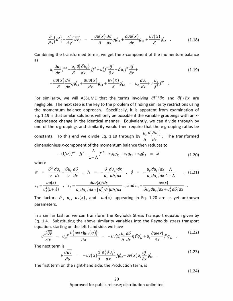
20 Approved for public release; distribution unlimited
{ } { } ( ) ( ) ( )211 11 12 .
uu x duu x uv xdu uv g g gx y dx dx∂ ∂ δ η∂ ∂ δ δ
′ ′+ = − + +
Combining the transformed terms, we get the x-component of the momentum balance as
{ }
( ) ( ) ( )
2 2
11 11 12 2 .
ss ss s s
e se
d udu u f fu f ff u f u fdx dx x x
uu x duu x uv x du ud g g g u fdx dx dx
δδ
δ
δ η νδ δ δ
′∂ ∂′ ′′ ′ ′′− + − +∂ ∂
′ ′ ′′′− + + = +
For similarity, we will ASSUME that the terms involving /′∂ ∂f x and /∂ ∂f x are negligible. The next step is the key to the problem of finding similarity restrictions using the momentum balance approach. Specifically, it is apparent from examination of Eq. 1.19 is that similar solutions will only be possible if the variable groupings with an x-dependence change in the identical manner. Equivalently, we can divide through by one of the x-groupings and similarity would then require that the x-grouping ratios be
constants. To this end we divide Eq. 1.19 through by { }ss d uudxδ
δ. The transformed
dimensionless x-component of the momentum balance then reduces to 2
1 11 2 11 3 12(1 )1
f ff f g g gα τ η τ τ φΛ′′′ ′′ ′ ′ ′− − − − + + =−Λ
where
( )
2
1 2 32 22
, , ,1
( )( ) ( ), , and .(1 )
s e es s
s s s
s s s ss s s
du dx u du dxdu u ddx dx u d dx u du dx
duu x dxuu x uv xu u du dx u d dxu du dx u d dx
δδ δ δα φν ν δ
τ τ τλ δ δδ δ
Λ= + Λ = − = −
−Λ
= = =+ ++
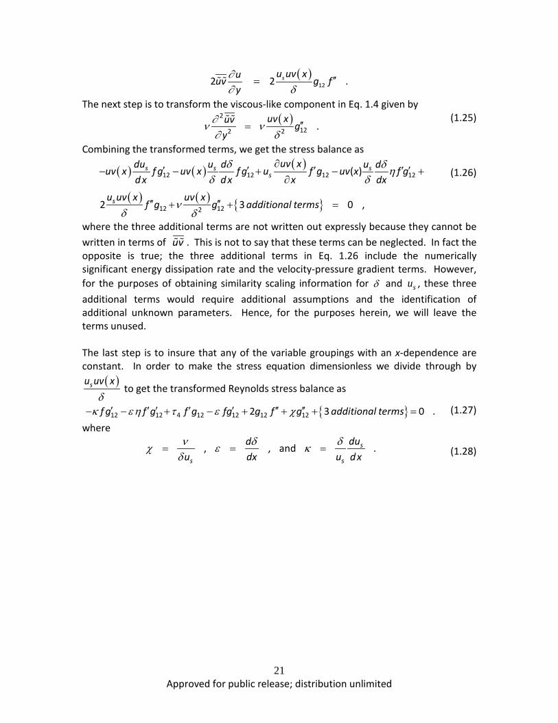
The factors δ , su , ( )uv x , and ( )uu x appearing in Eq. 1.20 are as yet unknown parameters. In a similar fashion we can transform the Reynolds Stress Transport equation given by Eq. 1.4. Substituting the above similarity variables into the Reynolds stress transport equation, starting on the left-hand side, we have
( ){ }1212 12
( ) ( )( ) .s
s s
uv x g uv xuuv du u f uv x f g u f gx x dx x
η∂ δ η∂ δ
∂ ∂′ ′ ′ ′= = − +∂ ∂
The next term is
( ) { } ( )12 121 .s
s
d uuv fv uv x fg uv x u gy d x x
δ∂∂ δ
∂′ ′= − −∂
The first term on the right-hand side, the Production term, is
(1.18)
(1.19)
(1.20)
(1.21)
(1.22)
(1.23)
(1.24)
21 Approved for public release; distribution unlimited
( )122 2 .su uv xuuv g f
y∂∂ δ
′′=
The next step is to transform the viscous-like component in Eq. 1.4 given by ( )2
122 2 .uv xuv g
y∂ν ν∂ δ
′′=
Combining the transformed terms, we get the stress balance as
( ) ( ) ( )
( ) ( ) { }
12 12 12 12
12 122
( )
2 3 0 ,
s s ss
s
uv xdu du u duv x f g uv x f g u f g uv x f gd x d x x dx
u uv x uv xf g g additional terms
δ δ ηδ δ
νδ δ
∂′ ′ ′ ′ ′− − + − +
∂
′′ ′′+ + =
where the three additional terms are not written out expressly because they cannot be written in terms of uv . This is not to say that these terms can be neglected. In fact the opposite is true; the three additional terms in Eq. 1.26 include the numerically significant energy dissipation rate and the velocity-pressure gradient terms. However, for the purposes of obtaining similarity scaling information for δ and su , these three additional terms would require additional assumptions and the identification of additional unknown parameters. Hence, for the purposes herein, we will leave the terms unused. The last step is to insure that any of the variable groupings with an x-dependence are constant. In order to make the stress equation dimensionless we divide through by
( )su uv xδ
to get the transformed Reynolds stress balance as
{ }12 12 4 12 12 12 122 3 0 .f g f g f g fg g f g additional termsκ εη τ ε χ′ ′ ′ ′ ′ ′′ ′′− − + − + + + = where
, , and .s
s s
dudu dx u d xν δ δχ ε κδ
= = =
(1.25)
(1.26)
(1.27)
(1.28)

![User profile correlation-based similarity (UPCSim) algorithm ......collaborative ltering similarity [29], the Triangle Multiplying Jaccard (TMJ) similarity [30], and the similarity](https://img.pdfslide.net/doc/110x75/6147013af4263007b1358a2c/user-profile-correlation-based-similarity-upcsim-algorithm-collaborative.jpg)