Transportation Research Part C 48 (2014) 158–171

Contents lists available at ScienceDirect

Transportation Research Part C

journal homepage: www.elsevier .com/locate / t rc

Evaluation of the effectiveness of accident information onfreeway changeable message signs: A comparison of empiricalmethodologies

http://dx.doi.org/10.1016/j.trc.2014.08.0110968-090X/� 2014 Elsevier Ltd. All rights reserved.

⇑ Corresponding author.E-mail addresses: xuanyg@berkeley.edu (Y. Xuan), kanafani@berkeley.edu (A. Kanafani).

Yiguang (Ethan) Xuan ⇑, Adib KanafaniInstitute of Transportation Studies, University of California, Berkeley, CA 94720, USA

a r t i c l e i n f o

Article history:Received 27 February 2014Received in revised form 30 May 2014Accepted 14 August 2014

Keywords:EmpiricalDriver behaviorChangeable message signAccidentVisible congestion

a b s t r a c t

In this paper, we study the effectiveness of accident messages that are displayed on free-way changeable message signs (CMS). Motivated by the lack of empirical studies and themixed results reported in the limited empirical studies, this paper focuses on the compar-ison of different aggregate analysis methodologies and their corresponding results, usingthe same empirical data set. We have two major findings. First, we find that the CMS acci-dent messages do not seem to have any significant immediate effect on driver diversionbased on our empirical data. Visible congestion, on the other hand, seems to be an impor-tant factor for driver diversion. Second, we show how the conclusion could have been ifwrong methodologies were to be adopted. Methods that rely on correlation alone butnot the timing of events (what we call correlation method) yield high correlation betweenCMS accident messages and driver diversion, which is typically and incorrectly interpretedas CMS accident messages being effective.

� 2014 Elsevier Ltd. All rights reserved.

1. Introduction

In this paper, we use empirical data to evaluate drivers’ response to messages displayed on freeway changeable messagesigns (CMS, also known as variable message signs or dynamic message signs).

We are generally interested in the effect of information on traveler behavior. As a starting point, we focus on the infor-mation conveyed through freeway CMS for two reasons. First, CMS has been in use in the field for a long time, at least sincethe 1960s. Second, the CMS system is expensive: Typical installation cost is around $200,000 for each freeway CMS, exclud-ing the cost for operation and maintenance. In California alone, there are about 771 such signs on the freeway, which cost atleast $150 million for installation. Therefore, we would like to understand the worth of this system.

However, we have very limited understanding of how effective CMS messages are. According to a recently publishedNCHRP report (Robinson et al., 2012), only 30 percent of the agencies reported having evaluation data that demonstratethe benefits of providing information to the traveling public, and only 40 percent have an ongoing program for evaluatingthe provision of traveler information. To most public agencies, the empirical effect of CMS is largely anecdotal and difficultto quantify. Most of the literature on the effect of CMS, as described in the next section, is based on stated preference surveysor simulations. Therefore, there is a need to study the effect of CMS with empirical data.

Y. Xuan, A. Kanafani / Transportation Research Part C 48 (2014) 158–171 159

2. Literature review

The literature on the effect of CMS is summarized into the following categories:

2.1. Idealized assumptions

Earlier efforts to quantify the effect of traveler information (Kanafani and Al-Deek, 1991; Al-Deek and Kanafani, 1993)tend to make idealized assumptions about driver response, for example that drivers will fully comply with route diversionsuggestions, either for system optimal assignment or to avoid incidents. The purpose of these studies is typically not tomodel driver response accurately, but rather to estimate the upper bound of the benefit of traveler information.

2.2. Stated preference surveys or simulations

The most commonly used method to study the effect of CMS is stated preference (SP) surveys (Khattak et al., 1993;Mannering et al., 1994; Madanat et al., 1995; Benson, 1996; Emmerink et al., 1996; Polydoropoulou et al., 1996;Wardman et al., 1997; Abdel-Aty et al., 1997; Peeta et al., 2000; Lappin and Bottom, 2001; Abdel-Aty and Abdalla, 2004;Chatterjee and Mcdonald, 2004; Chorus et al., 2006; Ben-Elia et al., 2013; Razo and Gao, 2013). Lappin and Bottom(2001), Chorus et al. (2006) provide good literature review on the findings from SP surveys. Typically, participants are askedwhat they would do if they see certain CMS messages. SP survey is an effective method to obtain information from individ-uals on their thought process. These and many other studies have offered insights into factors that affect drivers’ decision forroute diversion, including purpose of travel, schedule flexibility, travel distance, cause of congestion on current route, famil-iarity with alternative routes, information availability on alternative routes, and previous experiences with travelerinformation.

Studies using driving simulator (Dutta et al., 2004; Chorus et al., 2007, 2013) provide a comparatively more realistic set-ting to identify factors that affect the readability of information as well as the behavior of drivers. For example, Dutta et al.(2004) identifies the following factors that significant affect driver performance: visual obstructions of message signs, thedisplaying sequence of content, the message content, and the number and direction of lane changes required.

However, travelers’ stated preference (or their behavior in the driving simulator) can be different from their actual behav-ior, due to the lack of commitment. For example, Xu et al. (2011) finds that SP survey overestimates the number of driverswho take diversion routes. Therefore, results obtained through SP surveys or simulations may not be appropriate for oper-ational applications. For example, if CMS is used to divert traffic to arterial streets, the amount of traffic diverted needs to beestimated so that traffic signals on local streets can account for it. SP methods generally do not provide the level of accuracyneeded for such operational purposes.

2.3. Empirical data

Alternatively, one can study the effect of CMS with empirical data to see what travelers actually did. This is the approachtaken in this paper. The number of studies we are aware of in this category is much smaller compared with those using SPmethods, and these studies are summarized in Table 1.

We find that the effect of CMS reported by these studies varies over a wide range. While almost all the studies report theeffect of CMS to be statistically significant, the magnitude can sometimes be small and insignificant for operational purposes,such as in Dudek et al. (1982). Of course, the mixed results could be due to the differences in site location. But we also iden-tify two problems in the methodologies adopted by these studies, which we think contribute to the mixed results.

The first problem is that many studies regard CMS as the only information source, while failing to account for the poten-tial effect of visible congestion. However, the effect of visible congestion on diversion is well documented (Dudek et al., 1982;Ullman, 1992, 1996; Bushman et al., 2004; Liu et al., 2011; Wu et al., 2011; Xu et al., 2011). It has been empirically observedthat many drivers change their routes when serious congestion is visible, and visible congestion is potentially the explana-tion for the observation in Foo et al. (2008) that sometimes the turning rate changes before the message changes.

The second problem is in the method used to derive the effect of CMS. Two types of methods are mainly used in the lit-erature. The first method compares driver behavior with and without CMS messages, which we will call the correlationmethod. The second method compares the behavior right before and after CMS message changes, which we will call the cau-sality method. The correlation method is more likely to capture a mixed effect from various information sources, while thecausality methods is more likely to reveal the effect of CMS.1

As a summary, the number of empirical studies on the effect of CMS is small. Of the limited empirical studies, the reportedeffect of CMS varies greatly. Besides difference in site location, we speculate the mixed results can also be attributed to thedifferent methodologies adopted by the studies. The comparison between methodologies has not been done to our knowl-edge, and typically only one methodology is adopted by each study.

1 Strictly speaking, the term causality is too strong for the second method. In addition to correlation, the second method accounts for the timing of the events,which is a necessary but not sufficient condition for causality.

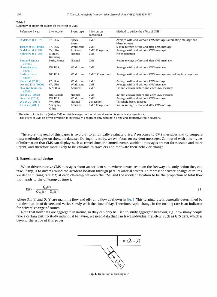
Table 1Summary of empirical studies on the effect of CMS.

Reference & year Site location Event type Info sourcesconsidered

Method to derive the effect of CMS

Dudek et al. (1978) TX, USA Specialevents

CMS⁄ Average with and without CMS message (alternating message andblank screen)

Turner et al. (1978) TX, USA Work zone CMS⁄ 5-min average before and after CMS messageDudek et al. (1982) TX, USA Accident CMS⁄ Congestion⁄ Average with and without CMS messageKuhne et al. (1996) Munich,

GermanyNormal CMS⁄ No explanation

Yim and Ygnace(1996)

Paris, France Normal CMS⁄ 5-min average before and after CMS message

Horowitz et al.(2003)

WI, USA Work zone CMS⁄ Average with and without CMS message

Bushman et al.(2004)

NC, USA Work zone CMS⁄⁄ Congestion⁄ Average with and without CMS message, controlling for congestion

Chu et al. (2005) CA, USA Work zone CMS⁄ Average with and without CMS messageLee and Kim (2006) CA, USA Work zone CMS⁄ Average with and without CMS messageHuo and Levinson

(2006)MN, USA Accident CMS⁄ 10-min average before and after CMS message

Foo et al. (2008) ON, Canada Normal CMS⁄ 30-min average before and after CMS messageLiu et al. (2011) WI, USA Work zone CMS⁄ Average with and without CMS messageWu et al. (2011) WA, USA Normal Congestion⁄ Threshold based methodXu et al. (2011) Shanghai,

ChinaAccident CMS⁄ Congestion⁄ 5-min average before and after CMS message

⁄ The effect of this factor (either CMS or visible congestion) on driver diversion is statistically significant.⁄⁄ The effect of CMS on driver diversion is statistically significant only with both delay and alternative route advisory.

160 Y. Xuan, A. Kanafani / Transportation Research Part C 48 (2014) 158–171

Therefore, the goal of this paper is twofold: to empirically evaluate drivers’ response to CMS messages and to comparethese methodologies on the same data set. During this study, we will focus on accident messages. Compared with other typesof information that CMS can display, such as travel time or planned events, accident messages are not foreseeable and moreurgent, and therefore more likely to be valuable to travelers and motivate their behavior change.

3. Experimental design

When drivers receive CMS messages about an accident somewhere downstream on the freeway, the only action they cantake, if any, is to divert around the accident location through parallel arterial streets. To represent drivers’ change of routes,we define turning rate RðtÞ at each off-ramp between the CMS and the accident location to be the proportion of total flowthat heads to the off-ramp at time t:

RðtÞ ¼ QRðtÞQ MLðtÞ þ Q RðtÞ

; ð1Þ

where Q MLðtÞ and Q RðtÞ are mainline flow and off-ramp flow as shown in Fig. 1. This turning rate is generally determined bythe destination of drivers and varies slowly with the time of day. Therefore, rapid change in the turning rate is an indicatorfor drivers’ change of routes.

Note that flow data are aggregate in nature, so they can only be used to study aggregate behavior, e.g., how many peopletake a certain exit. To study individual behavior, we need data that can trace individual travelers, such as GPS data, which isbeyond the scope of this paper.

Fig. 1. Definition of turning rate.

Y. Xuan, A. Kanafani / Transportation Research Part C 48 (2014) 158–171 161

3.1. Sites

Because of the data-driven nature of this study, the study sites are restricted to freeway sections that are well instru-mented with loop detectors, especially on the off-ramps. We try to select freeway sections that start with a freeway CMS,and have most of the downstream exits instrumented.

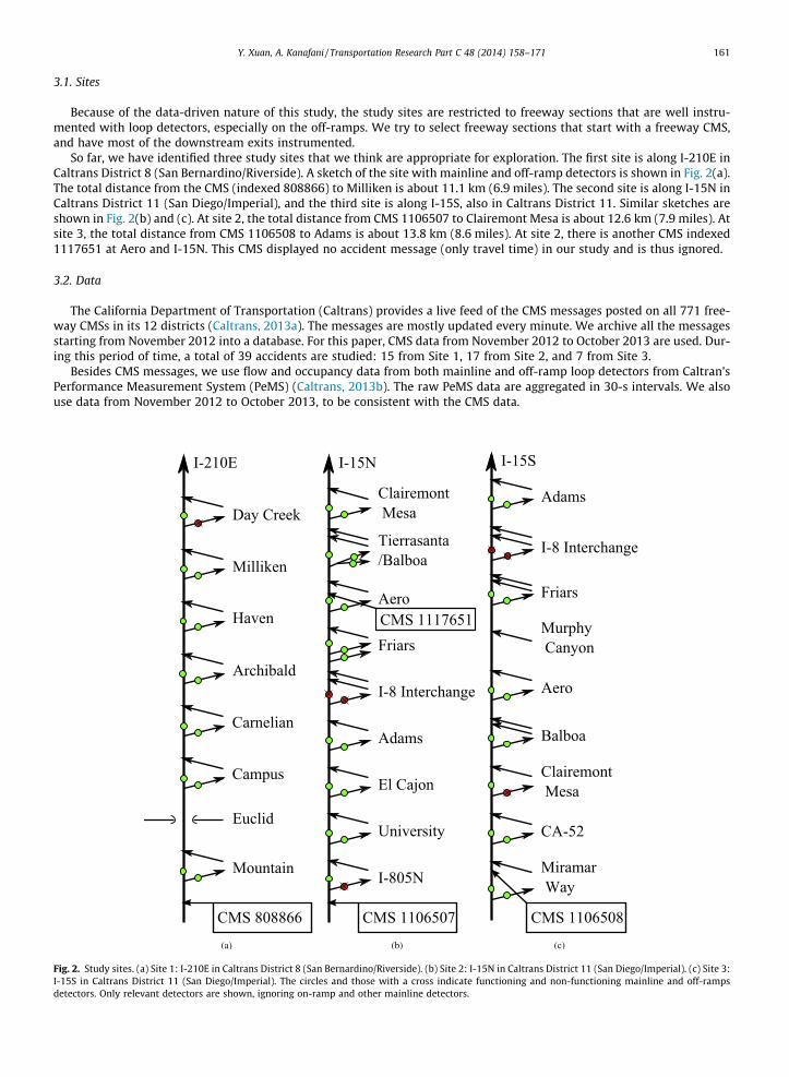
So far, we have identified three study sites that we think are appropriate for exploration. The first site is along I-210E inCaltrans District 8 (San Bernardino/Riverside). A sketch of the site with mainline and off-ramp detectors is shown in Fig. 2(a).The total distance from the CMS (indexed 808866) to Milliken is about 11.1 km (6.9 miles). The second site is along I-15N inCaltrans District 11 (San Diego/Imperial), and the third site is along I-15S, also in Caltrans District 11. Similar sketches areshown in Fig. 2(b) and (c). At site 2, the total distance from CMS 1106507 to Clairemont Mesa is about 12.6 km (7.9 miles). Atsite 3, the total distance from CMS 1106508 to Adams is about 13.8 km (8.6 miles). At site 2, there is another CMS indexed1117651 at Aero and I-15N. This CMS displayed no accident message (only travel time) in our study and is thus ignored.

3.2. Data

The California Department of Transportation (Caltrans) provides a live feed of the CMS messages posted on all 771 free-way CMSs in its 12 districts (Caltrans, 2013a). The messages are mostly updated every minute. We archive all the messagesstarting from November 2012 into a database. For this paper, CMS data from November 2012 to October 2013 are used. Dur-ing this period of time, a total of 39 accidents are studied: 15 from Site 1, 17 from Site 2, and 7 from Site 3.

Besides CMS messages, we use flow and occupancy data from both mainline and off-ramp loop detectors from Caltran’sPerformance Measurement System (PeMS) (Caltrans, 2013b). The raw PeMS data are aggregated in 30-s intervals. We alsouse data from November 2012 to October 2013, to be consistent with the CMS data.

Fig. 2. Study sites. (a) Site 1: I-210E in Caltrans District 8 (San Bernardino/Riverside). (b) Site 2: I-15N in Caltrans District 11 (San Diego/Imperial). (c) Site 3:I-15S in Caltrans District 11 (San Diego/Imperial). The circles and those with a cross indicate functioning and non-functioning mainline and off-rampsdetectors. Only relevant detectors are shown, ignoring on-ramp and other mainline detectors.

162 Y. Xuan, A. Kanafani / Transportation Research Part C 48 (2014) 158–171

4. Case studies

We start our analysis with two case studies to draw insights into the effect of CMS on driver diversion.

4.1. Case study 1

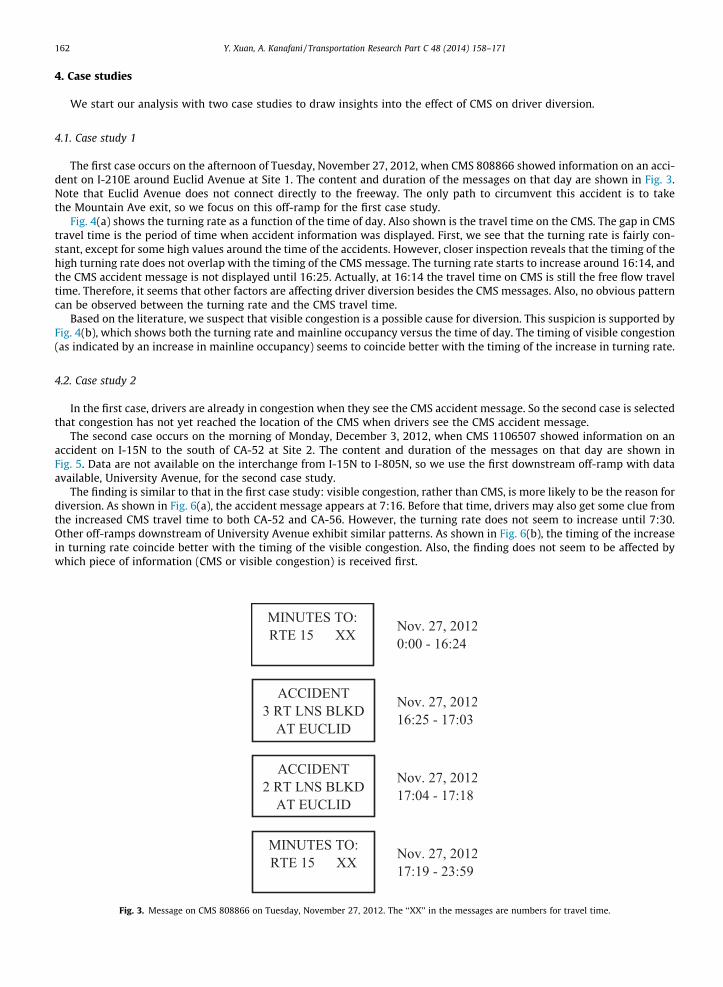
The first case occurs on the afternoon of Tuesday, November 27, 2012, when CMS 808866 showed information on an acci-dent on I-210E around Euclid Avenue at Site 1. The content and duration of the messages on that day are shown in Fig. 3.Note that Euclid Avenue does not connect directly to the freeway. The only path to circumvent this accident is to takethe Mountain Ave exit, so we focus on this off-ramp for the first case study.

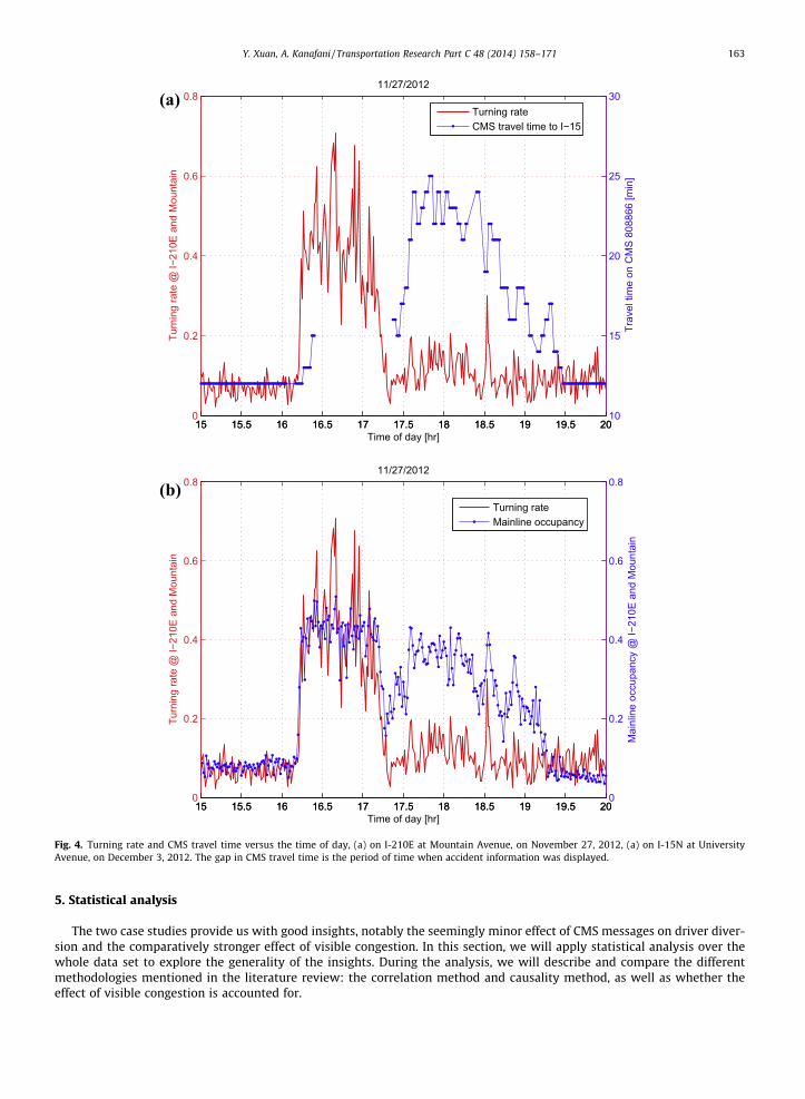
Fig. 4(a) shows the turning rate as a function of the time of day. Also shown is the travel time on the CMS. The gap in CMStravel time is the period of time when accident information was displayed. First, we see that the turning rate is fairly con-stant, except for some high values around the time of the accidents. However, closer inspection reveals that the timing of thehigh turning rate does not overlap with the timing of the CMS message. The turning rate starts to increase around 16:14, andthe CMS accident message is not displayed until 16:25. Actually, at 16:14 the travel time on CMS is still the free flow traveltime. Therefore, it seems that other factors are affecting driver diversion besides the CMS messages. Also, no obvious patterncan be observed between the turning rate and the CMS travel time.

Based on the literature, we suspect that visible congestion is a possible cause for diversion. This suspicion is supported byFig. 4(b), which shows both the turning rate and mainline occupancy versus the time of day. The timing of visible congestion(as indicated by an increase in mainline occupancy) seems to coincide better with the timing of the increase in turning rate.

4.2. Case study 2

In the first case, drivers are already in congestion when they see the CMS accident message. So the second case is selectedthat congestion has not yet reached the location of the CMS when drivers see the CMS accident message.

The second case occurs on the morning of Monday, December 3, 2012, when CMS 1106507 showed information on anaccident on I-15N to the south of CA-52 at Site 2. The content and duration of the messages on that day are shown inFig. 5. Data are not available on the interchange from I-15N to I-805N, so we use the first downstream off-ramp with dataavailable, University Avenue, for the second case study.

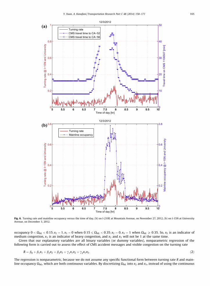
The finding is similar to that in the first case study: visible congestion, rather than CMS, is more likely to be the reason fordiversion. As shown in Fig. 6(a), the accident message appears at 7:16. Before that time, drivers may also get some clue fromthe increased CMS travel time to both CA-52 and CA-56. However, the turning rate does not seem to increase until 7:30.Other off-ramps downstream of University Avenue exhibit similar patterns. As shown in Fig. 6(b), the timing of the increasein turning rate coincide better with the timing of the visible congestion. Also, the finding does not seem to be affected bywhich piece of information (CMS or visible congestion) is received first.

Fig. 3. Message on CMS 808866 on Tuesday, November 27, 2012. The ‘‘XX’’ in the messages are numbers for travel time.

15 15.5 16 16.5 17 17.5 18 18.5 19 19.5 200

0.2

0.4

0.6

0.8

Time of day [hr]

Turn

ing

rate

@ I−

210E

and

Mou

ntai

n

15 15.5 16 16.5 17 17.5 18 18.5 19 19.5 2010

15

20

25

30

Trav

el ti

me

on C

MS

8088

66 [m

in]

11/27/2012

Turning rateCMS travel time to I−15

(a)

15 15.5 16 16.5 17 17.5 18 18.5 19 19.5 200

0.2

0.4

0.6

0.8

Time of day [hr]

Turn

ing

rate

@ I−

210E

and

Mou

ntai

n

15 15.5 16 16.5 17 17.5 18 18.5 19 19.5 200

0.2

0.4

0.6

0.8

Mai

nlin

e oc

cupa

ncy

@ I−

210E

and

Mou

ntai

n

11/27/2012

Turning rateMainline occupancy

(b)

Fig. 4. Turning rate and CMS travel time versus the time of day, (a) on I-210E at Mountain Avenue, on November 27, 2012, (a) on I-15N at UniversityAvenue, on December 3, 2012. The gap in CMS travel time is the period of time when accident information was displayed.

Y. Xuan, A. Kanafani / Transportation Research Part C 48 (2014) 158–171 163

5. Statistical analysis

The two case studies provide us with good insights, notably the seemingly minor effect of CMS messages on driver diver-sion and the comparatively stronger effect of visible congestion. In this section, we will apply statistical analysis over thewhole data set to explore the generality of the insights. During the analysis, we will describe and compare the differentmethodologies mentioned in the literature review: the correlation method and causality method, as well as whether theeffect of visible congestion is accounted for.

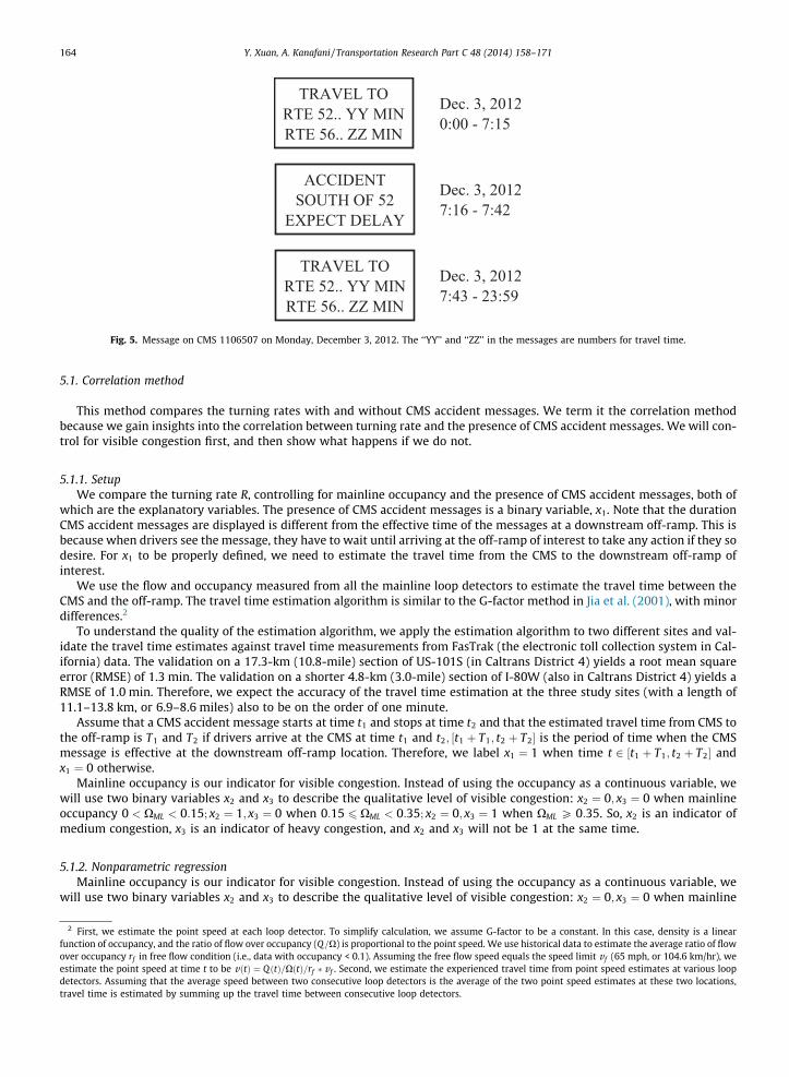
Fig. 5. Message on CMS 1106507 on Monday, December 3, 2012. The ‘‘YY’’ and ‘‘ZZ’’ in the messages are numbers for travel time.

164 Y. Xuan, A. Kanafani / Transportation Research Part C 48 (2014) 158–171

5.1. Correlation method

This method compares the turning rates with and without CMS accident messages. We term it the correlation methodbecause we gain insights into the correlation between turning rate and the presence of CMS accident messages. We will con-trol for visible congestion first, and then show what happens if we do not.

5.1.1. SetupWe compare the turning rate R, controlling for mainline occupancy and the presence of CMS accident messages, both of

which are the explanatory variables. The presence of CMS accident messages is a binary variable, x1. Note that the durationCMS accident messages are displayed is different from the effective time of the messages at a downstream off-ramp. This isbecause when drivers see the message, they have to wait until arriving at the off-ramp of interest to take any action if they sodesire. For x1 to be properly defined, we need to estimate the travel time from the CMS to the downstream off-ramp ofinterest.

We use the flow and occupancy measured from all the mainline loop detectors to estimate the travel time between theCMS and the off-ramp. The travel time estimation algorithm is similar to the G-factor method in Jia et al. (2001), with minordifferences.2

To understand the quality of the estimation algorithm, we apply the estimation algorithm to two different sites and val-idate the travel time estimates against travel time measurements from FasTrak (the electronic toll collection system in Cal-ifornia) data. The validation on a 17.3-km (10.8-mile) section of US-101S (in Caltrans District 4) yields a root mean squareerror (RMSE) of 1.3 min. The validation on a shorter 4.8-km (3.0-mile) section of I-80W (also in Caltrans District 4) yields aRMSE of 1.0 min. Therefore, we expect the accuracy of the travel time estimation at the three study sites (with a length of11.1–13.8 km, or 6.9–8.6 miles) also to be on the order of one minute.

Assume that a CMS accident message starts at time t1 and stops at time t2 and that the estimated travel time from CMS tothe off-ramp is T1 and T2 if drivers arrive at the CMS at time t1 and t2; ½t1 þ T1; t2 þ T2� is the period of time when the CMSmessage is effective at the downstream off-ramp location. Therefore, we label x1 ¼ 1 when time t 2 ½t1 þ T1; t2 þ T2� andx1 ¼ 0 otherwise.

Mainline occupancy is our indicator for visible congestion. Instead of using the occupancy as a continuous variable, wewill use two binary variables x2 and x3 to describe the qualitative level of visible congestion: x2 ¼ 0; x3 ¼ 0 when mainlineoccupancy 0 < XML < 0:15; x2 ¼ 1; x3 ¼ 0 when 0:15 6 XML < 0:35; x2 ¼ 0; x3 ¼ 1 when XML P 0:35. So, x2 is an indicator ofmedium congestion, x3 is an indicator of heavy congestion, and x2 and x3 will not be 1 at the same time.

5.1.2. Nonparametric regressionMainline occupancy is our indicator for visible congestion. Instead of using the occupancy as a continuous variable, we

will use two binary variables x2 and x3 to describe the qualitative level of visible congestion: x2 ¼ 0; x3 ¼ 0 when mainline

2 First, we estimate the point speed at each loop detector. To simplify calculation, we assume G-factor to be a constant. In this case, density is a linearfunction of occupancy, and the ratio of flow over occupancy (Q=X) is proportional to the point speed. We use historical data to estimate the average ratio of flowover occupancy rf in free flow condition (i.e., data with occupancy < 0.1). Assuming the free flow speed equals the speed limit v f (65 mph, or 104.6 km/hr), weestimate the point speed at time t to be vðtÞ ¼ QðtÞ=XðtÞ=rf � v f . Second, we estimate the experienced travel time from point speed estimates at various loopdetectors. Assuming that the average speed between two consecutive loop detectors is the average of the two point speed estimates at these two locations,travel time is estimated by summing up the travel time between consecutive loop detectors.

5 5.5 6 6.5 7 7.5 8 8.5 9 9.5 100

0.2

0.4

0.6

0.8

1

Time of day [hr]

Turn

ing

rate

@ I−

15N

and

Uni

vers

ity

12/3/2012

5 5.5 6 6.5 7 7.5 8 8.5 9 9.5 100

10

20

30

40

50

Trav

el ti

me

on C

MS

1106

507

[min

]

Turning rateCMS travel time to CA−52CMS travel time to CA−56

(a)

5 5.5 6 6.5 7 7.5 8 8.5 9 9.5 100

0.2

0.4

0.6

0.8

Time of day [hr]

Turn

ing

rate

@ I−

15N

and

Uni

vers

ity

12/3/2012

5 5.5 6 6.5 7 7.5 8 8.5 9 9.5 100

0.2

0.4

0.6

0.8

Mai

nlin

e oc

cupa

ncy

@ I−

15N

and

Uni

vers

ity

Turning rateMainline occupancy

(b)

Fig. 6. Turning rate and mainline occupancy versus the time of day, (b) on I-210E at Mountain Avenue, on November 27, 2012, (b) on I-15N at UniversityAvenue, on December 3, 2012.

Y. Xuan, A. Kanafani / Transportation Research Part C 48 (2014) 158–171 165

occupancy 0 < XML < 0:15; x2 ¼ 1; x3 ¼ 0 when 0:15 6 XML < 0:35; x2 ¼ 0; x3 ¼ 1 when XML P 0:35. So, x2 is an indicator ofmedium congestion, x3 is an indicator of heavy congestion, and x2 and x3 will not be 1 at the same time.

Given that our explanatory variables are all binary variables (or dummy variables), nonparametric regression of thefollowing form is carried out to assess the effect of CMS accident messages and visible congestion on the turning rate

R ¼ b0 þ b1x1 þ b2x2 þ b2x3 þ c1x1x2 þ c2x1x3: ð2Þ

The regression is nonparametric, because we do not assume any specific functional form between turning rate R and main-line occupancy XML, which are both continuous variables. By discretizing XML into x2 and x3, instead of using the continuous

166 Y. Xuan, A. Kanafani / Transportation Research Part C 48 (2014) 158–171

variable, the model only estimate the level but not the slope. The interaction terms x1x2 and x1x3 are added to account for thecorrelation between explanatory variables.

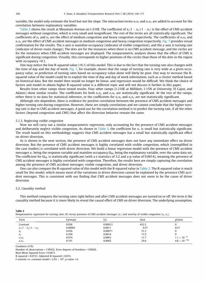
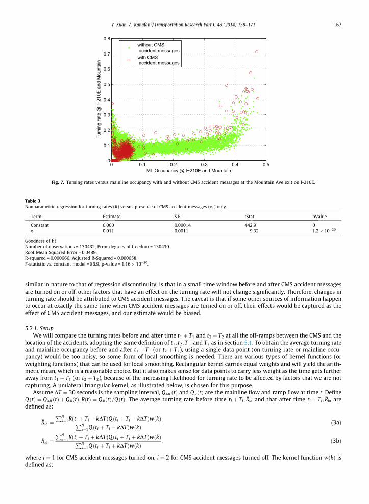
Table 2 shows the result at Mountain Avenue on I-210E. The coefficient of x1ð1� x2Þð1� x3Þ is the effect of CMS accidentmessages without congestion, which is very small and insignificant. The rest of the terms are all statistically significant. Thecoefficients of x2 and x3 are the effect of medium congestion and heavy congestion respectively. The coefficients of x1x2 andx1x3 are the effect of CMS accident messages in medium congestion and heavy congestion respectively. Fig. 7 provides visualconfirmation for the results. The x-axis is mainline occupancy (indicator of visible congestion), and the y-axis is turning rate(indicator of driver route change). The dots are for the instances when there is no CMS accident message, and the circles arefor the instances when CMS accident messages are displayed. The nonparametric analysis shows that the effect of CMS issignificant during congestion. Visually, this corresponds to higher positions of the circles than those of the dots in the regionwith occupancy >0.1.

One may notice the low R-squared value (<0.1) of this model. This is due to the fact that the turning rate also changes withthe time of day and the day of week. Fig. 7, for example, shows that the range of turning rate is very wide at a given occu-pancy value, so prediction of turning rates based on occupancy value alone will likely be poor. One way to increase the R-squared value of the model could be to exploit the time of day and day of week information, such as a cluster method basedon historical data. But the model then would no longer be linear, and regression would be difficult. We think the choice offactors and model to obtain higher R-squared value is a different topic and will not discuss it further in this paper.

Results from other ramps show mixed results. Four other ramps (I-210E at Milliken; I-15N at University, El Cajon, andAdams) show similar results: The coefficients for both x1x2 and x1x3 are statistically significant. At the rest of the ramps,either there is no data for statistical inference, or the coefficients for x1x2 and x1x3 are not statistically significant.

Although site-dependent, there is evidence for positive correlation between the presence of CMS accident messages andhigher turning rate during congestion. However, these are simply correlations and we cannot conclude that the higher turn-ing rate is due to CMS accident messages. A good use for the correlation method is to predict the turning rate, if all the otherfactors (beyond congestion and CMS) that affect the diversion behavior remain the same.

5.1.3. Neglecting visible congestionNow we will carry out a similar nonparametric regression, only accounting for the presence of CMS accident messages

and deliberately neglect visible congestion. As shown in Table 3, the coefficient for x1 is small but statistically significant.The result based on this methodology suggests that CMS accident messages has a small but statistically significant effecton driver diversion.

As is shown in the next section, the presence of CMS accident messages does not have any immediate effect on driverdiversion. But the presence of CMS accident messages is highly correlated with visible congestion, which (exemplified inthe case studies) is correlated with driver diversion. We build a linear regression model with the presence of CMS accidentmessages x1 being the response variable and mainline occupancy XML being the explanatory variable, over the same data set.The coefficient for XML is statistically significant (with a t-statistics of 3.2 and a p-value of 0.0014), meaning the presence ofCMS accident messages is highly correlated with congestion. Therefore, the results here are simply capturing the correlationamong the presence of CMS accident messages, visible congestion, and driver diversion.

One can also compare the R-squared value of this model with the R-squared value in Table 2. The R-squared value is muchsmall for this model, which means most of the variations in driver diversion cannot be explained by the presence CMS acci-dent messages. This is consistent with our finding that CMS accident messages does not seem to be the cause of driverdiversion.

5.2. Causality method

This method compares the turning rates right before and after CMS accident messages are turned on or off. We term it thecausality method because it is more likely to reveal the causal effect of CMS on driver diversion. The underlying assumption,

Table 2Nonparametric regression for turning rates (R) versus presence of CMS accident messages (x1) and severity of visible congestion (x2 ; x3).

Term Estimate S.E. tStat pValue

Constant 0.058 0.00013 432.5 0x1ð1� x2Þð1� x3Þ 0.00065 0.0011 0.57 0.57x2 0.036 0.00071 51.2 0x3 0.104 0.0014 71.9 0x1x2 0.074 0.0063 11.7 1.1 � 10�31

x1x3 0.191 0.0065 29.6 4.8 � 10�192

Goodness of fit:Number of observations = 130432, Error degrees of freedom = 130426.Root Mean Squared Error = 0.0471.R-squared = 0.0721, Adjusted R-Squared = 0.072.F-statistic vs. constant model = 2.03 � 103, p-value = 0.

0 0.1 0.2 0.3 0.4 0.50

0.1

0.2

0.3

0.4

0.5

0.6

0.7

0.8

ML Occupancy @ I−210E and Mountain

Turn

ing

rate

@ I−

210E

and

Mou

ntai

n

without CMS accident messageswith CMS accident messages

Fig. 7. Turning rates versus mainline occupancy with and without CMS accident messages at the Mountain Ave exit on I-210E.

Table 3Nonparametric regression for turning rates (R) versus presence of CMS accident messages (x1) only.

Term Estimate S.E. tStat pValue

Constant 0.060 0.00014 442.9 0x1 0.011 0.0011 9.32 1.2 � 10�20

Goodness of fit:Number of observations = 130432, Error degrees of freedom = 130430.Root Mean Squared Error = 0.0489.R-squared = 0.000666, Adjusted R-Squared = 0.000658.F-statistic vs. constant model = 86.9, p-value = 1.16 � 10�20.

Y. Xuan, A. Kanafani / Transportation Research Part C 48 (2014) 158–171 167

similar in nature to that of regression discontinuity, is that in a small time window before and after CMS accident messagesare turned on or off, other factors that have an effect on the turning rate will not change significantly. Therefore, changes inturning rate should be attributed to CMS accident messages. The caveat is that if some other sources of information happento occur at exactly the same time when CMS accident messages are turned on or off, their effects would be captured as theeffect of CMS accident messages, and our estimate would be biased.

5.2.1. SetupWe will compare the turning rates before and after time t1 þ T1 and t2 þ T2 at all the off-ramps between the CMS and the

location of the accidents, adopting the same definition of t1; t2; T1, and T2 as in Section 5.1. To obtain the average turning rateand mainline occupancy before and after t1 þ T1 (or t2 þ T2), using a single data point (on turning rate or mainline occu-pancy) would be too noisy, so some form of local smoothing is needed. There are various types of kernel functions (orweighting functions) that can be used for local smoothing. Rectangular kernel carries equal weights and will yield the arith-metic mean, which is a reasonable choice. But it also makes sense for data points to carry less weight as the time gets furtheraway from t1 þ T1 (or t2 þ T2), because of the increasing likelihood for turning rate to be affected by factors that we are notcapturing. A unilateral triangular kernel, as illustrated below, is chosen for this purpose.

Assume DT ¼ 30 seconds is the sampling interval, QMLðtÞ and QRðtÞ are the mainline flow and ramp flow at time t. DefineQðtÞ ¼ Q MLðtÞ þ Q RðtÞ;RðtÞ ¼ Q RðtÞ=QðtÞ. The average turning rate before time ti þ Ti; �Rib and that after time ti þ Ti; �Ria aredefined as:

�Rib ¼PN

k¼1Rðti þ Ti � kDTÞQðti þ Ti � kDTÞwðkÞPNk¼1Qðti þ Ti � kDTÞwðkÞ

; ð3aÞ

�Ria ¼PN

k¼1Rðti þ Ti þ kDTÞQðti þ Ti þ kDTÞwðkÞPNk¼1Qðti þ Ti þ kDTÞwðkÞ

; ð3bÞ

where i ¼ 1 for CMS accident messages turned on, i ¼ 2 for CMS accident messages turned off. The kernel function wðkÞ isdefined as:

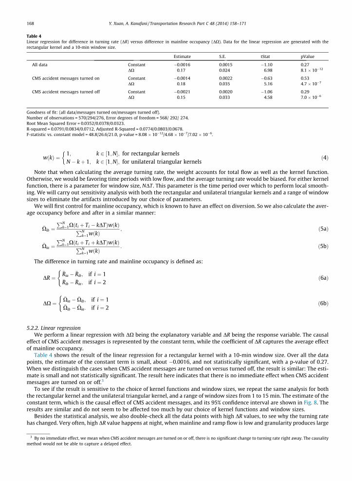
Table 4Linear regression for difference in turning rate (DR) versus difference in mainline occupancy (DX). Data for the linear regression are generated with therectangular kernel and a 10-min window size.

Estimate S.E. tStat pValue

All data Constant �0.0016 0.0015 �1.10 0.27DX 0.17 0.024 6.98 8.1 � 10�12

CMS accident messages turned on Constant �0.0014 0.0022 �0.63 0.53DX 0.18 0.035 5.16 4.7 � 10�7

CMS accident messages turned off Constant �0.0021 0.0020 �1.06 0.29DX 0.15 0.033 4.58 7.0 � 10�6

Goodness of fit: (all data/messages turned on/messages turned off).Number of observations = 570/294/276, Error degrees of freedom = 568/ 292/ 274.Root Mean Squared Error = 0.0352/0.0378/0.0323.R-squared = 0.0791/0.0834/0.0712, Adjusted R-Squared = 0.0774/0.0803/0.0678.F-statistic vs. constant model = 48.8/26.6/21.0, p-value = 8.08 � 10�12/4.68 � 10�7/7.02 � 10�6.

3 Bymethod

168 Y. Xuan, A. Kanafani / Transportation Research Part C 48 (2014) 158–171

wðkÞ ¼1; k 2 ½1;N�; for rectangular kernelsN � kþ 1; k 2 ½1;N�; for unilateral triangular kernels

�ð4Þ

Note that when calculating the average turning rate, the weight accounts for total flow as well as the kernel function.Otherwise, we would be favoring time periods with low flow, and the average turning rate would be biased. For either kernelfunction, there is a parameter for window size, NDT. This parameter is the time period over which to perform local smooth-ing. We will carry out sensitivity analysis with both the rectangular and unilateral triangular kernels and a range of windowsizes to eliminate the artifacts introduced by our choice of parameters.

We will first control for mainline occupancy, which is known to have an effect on diversion. So we also calculate the aver-age occupancy before and after in a similar manner:

�Xib ¼PN

k¼1Xðti þ Ti � kDTÞwðkÞPNk¼1wðkÞ

; ð5aÞ

�Xia ¼PN

k¼1Xðti þ Ti þ kDTÞwðkÞPNk¼1wðkÞ

: ð5bÞ

The difference in turning rate and mainline occupancy is defined as:

DR ¼�Ria � �Rib; if i ¼ 1�Rib � �Ria; if i ¼ 2

(ð6aÞ

DX ¼�Xia � �Xib; if i ¼ 1�Xib � �Xia: if i ¼ 2

(ð6bÞ

5.2.2. Linear regressionWe perform a linear regression with DX being the explanatory variable and DR being the response variable. The causal

effect of CMS accident messages is represented by the constant term, while the coefficient of DR captures the average effectof mainline occupancy.

Table 4 shows the result of the linear regression for a rectangular kernel with a 10-min window size. Over all the datapoints, the estimate of the constant term is small, about �0.0016, and not statistically significant, with a p-value of 0.27.When we distinguish the cases when CMS accident messages are turned on versus turned off, the result is similar: The esti-mate is small and not statistically significant. The result here indicates that there is no immediate effect when CMS accidentmessages are turned on or off.3

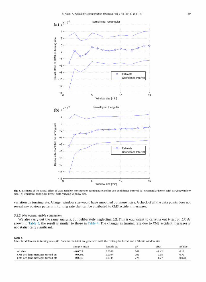
To see if the result is sensitive to the choice of kernel functions and window sizes, we repeat the same analysis for boththe rectangular kernel and the unilateral triangular kernel, and a range of window sizes from 1 to 15 min. The estimate of theconstant term, which is the causal effect of CMS accident messages, and its 95% confidence interval are shown in Fig. 8. Theresults are similar and do not seem to be affected too much by our choice of kernel functions and window sizes.

Besides the statistical analysis, we also double-check all the data points with high DR values, to see why the turning ratehas changed. Very often, high DR value happens at night, when mainline and ramp flow is low and granularity produces large

no immediate effect, we mean when CMS accident messages are turned on or off, there is no significant change to turning rate right away. The causalitywould not be able to capture a delayed effect.

0 5 10 15−14

−12

−10

−8

−6

−4

−2

0

2

4

6x 10−3

Window size [min]

Cau

sal e

ffect

of C

MS

on tu

rnin

g ra

te

kernel type: rectangular

EstimateConfidence Interval

(a)

0 5 10 15−16

−14

−12

−10

−8

−6

−4

−2

0

2

4x 10−3

Window size [min]

Cau

sal e

ffect

of C

MS

on tu

rnin

g ra

te

kernel type: triangular

EstimateConfidence Interval

(b)

Fig. 8. Estimate of the causal effect of CMS accident messages on turning rate and its 95% confidence interval. (a) Rectangular kernel with varying windowsize. (b) Unilateral triangular kernel with varying window size.

Y. Xuan, A. Kanafani / Transportation Research Part C 48 (2014) 158–171 169

variation on turning rate. A larger window size would have smoothed out more noise. A check of all the data points does notreveal any obvious pattern in turning rate that can be attributed to CMS accident messages.

5.2.3. Neglecting visible congestionWe also carry out the same analysis, but deliberately neglecting DX. This is equivalent to carrying out t-test on DR. As

shown in Table 5, the result is similar to those in Table 4: The changes in turning rate due to CMS accident messages isnot statistically significant.

Table 5T-test for difference in turning rate (DR). Data for the t-test are generated with the rectangular kernel and a 10-min window size.

Sample mean Sample std dF tStat pValue

All data �0.0022 0.0366 569 �1.42 0.16CMS accident messages turned on �0.00087 0.0394 293 �0.38 0.70CMS accident messages turned off �0.0036 0.0334 275 �1.77 0.078

170 Y. Xuan, A. Kanafani / Transportation Research Part C 48 (2014) 158–171

We also have figures like those in Fig. 8, by neglecting visible congestion. We did not show them here because they arealmost the same and the difference is too small to notice.

The reason for the little difference by neglecting visible congestion is likely that the mainline occupancy does not changemuch when CMS accident messages are turned on or off. This finding seems to support the assumption of the causalitymethod, that factors not captured by this method will not change significantly in a short time window before and afterCMS accident messages are turned on or off.

5.3. Findings

Based on our empirical data, we think it is safe to conclude that CMS accident messages do not seem to have any signif-icant immediate effect on driver diversion. The finding is consistent with our observations from the case studies, as well assome previous studies that are carefully carried out (Dudek et al., 1982; Bushman et al., 2004). Visible congestion, on theother hand, seems to be an important factor for driver diversion.

Another important contribution of this paper is the comparison of different methodologies over the same data set. Thecausality method, which is the correct one to use, shows that CMS accident messages do not seem to have any significantimmediate effect on driver diversion. The method is actually robust to whether visible congestion is accounted for or not.The correlation method identifies correlation between the presence of CMS accident messages and driver diversion duringcongestion. If this method is misused, one may incorrectly conclude that CMS accident messages are effective to driver diver-sion during congestion. If one further fails to account for the effect of visible congestion, the conclusion would be that CMSaccident messages have a small but statistically significant effect on driver diversion.

6. Conclusion and future research

This paper studies the empirical effect of accident messages conveyed through freeway changeable message sign (CMS)on driver diversion. The literature on the empirical effect of CMS is very limited. The few empirical studies we find reportmixed results, which we think is caused by the difference in site location as well as the various methodologies adoptedby these studies. The main contribution of this paper is twofold. First, we use empirical data to evaluate the effect of CMSaccident messages on driver diversion. Second, we compare the various methodologies using the same data set.

With case studies and statistical methods that focus on both correlation and the timing of events, we find that CMS acci-dent messages do not seem to have any significant immediate effect on driver diversion. This conclusion only applies to thethree study sites and the duration of data from November 2012 to October 2013, but it is consistent with some previousstudies that are carefully carried out (Dudek et al., 1982; Bushman et al., 2004). Visible congestion, on the other hand, seemsto be an important factor for driver diversion. We also show that with statistical analysis that only focuses on correlation,one may incorrectly conclude that CMS accident messages are effective to driver diversion during congestion. If one furtherfails to account for the effect of visible congestion, the conclusion would be that CMS accident messages have a small butstatistically significant effect on driver diversion.

There are a few possible directions for future research:

� The study obviously should be expanded to include more study sites, if data are available.� The CMS accident messages in this study are descriptive (i.e., where and what happened) in nature. There is some evi-

dence, in the literature and through our investigation, that prescriptive messages (i.e., CMS tells drivers to take certainroutes) are more effective. Although prescriptive CMS messages are much less frequent, their potential is worthinvestigating.� The flow data used in this study only provide insights into aggregated behavior represented by the change of turning

rates. GPS data carry much richer information on individual routes, and can help us better understand how drivers changetheir routes.

Acknowledgment

This research is funded by the California Department of Transportation under the Connected Corridors program.

References

Abdel-Aty, M., Abdalla, M., 2004. Modeling drivers’ diversion from normal routes under ATIS using generalized estimating equations and binomial probitlink function. Transportation 31, 327–348.

Abdel-Aty, M.A., Kitamura, R., Jovanis, P.P., 1997. Using stated preference data for studying the effect of advanced traffic information on drivers’ routechoice. Transp. Res. Part C: Emerging Technol. 5, 39–50.

Al-Deek, H., Kanafani, A., 1993. Modeling the benefits of advanced traveler information systems in corridors with incidents. Transp. Res. Part C: EmergingTechnol. 1, 303–324.

Ben-Elia, E., Pace, R.D., Bifulco, G.N., Shiftan, Y., 2013. The impact of travel information’s accuracy on route-choice. Transp. Res. Part C: Emerging Technol. 26,146–159.

Benson, B., 1996. Motorist attitudes about content of variable-message signs. Transp. Res. Rec. J. Transp. Res. Board 1550, 48–57.

Y. Xuan, A. Kanafani / Transportation Research Part C 48 (2014) 158–171 171

Bushman, R., Berthelot, C., Chan, J., 2004. Effects of a smart work zone on motorist route decisions. In: 2004 Annual Conference of the TransportationAssociation of Canada, pp. 1–11.

Caltrans, 2013a. Changeable Message Signs (CMS) Feed. <http://www.dot.ca.gov/cwwp2/documentation/cms/cms.htm>.Caltrans, 2013b. Performance Measurement System (PeMS). <http://pems.dot.ca.gov/>.Chatterjee, K., Mcdonald, M., 2004. Effectiveness of using variable message signs to disseminate dynamic traffic information: evidence from field trails in

european cities. Transp. Rev. 24, 559–585.Chorus, C.G., Molin, E.J., Arentze, T.A., Hoogendoorn, S.P., Timmermans, H.J., Wee, B.V., 2007. Validation of a multimodal travel simulator with travel

information provision. Transp. Res. Part C: Emerging Technol. 15, 191–207.Chorus, C.G., Molin, E.J., van Wee, B., 2006. Traveler information as an instrument to change car-drivers’ travel choices: a literature review. Eur. J. Transp.

Infrastruct. Res. 6, 335–364.Chorus, C.G., Walker, J.L., Ben-Akiva, M., 2013. A joint model of travel information acquisition and response to received messages. Transp. Res. Part C:

Emerging Technol. 26, 61–77.Chu, L., Kim, H.K., Chung, Y., Recker, W., 2005. Evaluation of effectiveness of automated work zone information systems. Transp. Res. Rec. J. Transp. Res.

Board 1911, 73–81.Dudek, C.L., Stokton, W.R., Hatcher, D.R., 1982. Real-time freeway-to-freeway diversion: the san antonio experience. Transp. Res. Rec. J. Transp. Res. Board

841, 1–14.Dudek, C.L., Weaver, G.D., Hatcher, D.R., Richards, S.H., 1978. Field evaluation of messages for real-time diversion of freeway traffic for special events.

Transp. Res. Rec. J. Transp. Res. Board 682, 37–45.Dutta, A., Fisher, D.L., Noyce, D.A., 2004. Use of a driving simulator to evaluate and optimize factors affecting understandability of variable message signs.

Transp. Res. Part F: Traffic Psychol. Behav. 7, 209–227.Emmerink, R.H., Nijkamp, P., Rietveld, P., Ommeren, J.N.V., 1996. Variable message signs and radio traffic information: an integrated empirical analysis of

drivers’ route choice behaviour. Transp. Res. Part A: Policy Pract. 30, 135–153.Foo, S., Abdulhai, B., Hall, F., 2008. Impacts on traffic diversion rates of changed message on changeable message sign. Transp. Res. Rec. J. Transp. Res. Board

2047, 11–18.Horowitz, A., Weisser, I., Notbohm, T., 2003. Diversion from a rural work zone with traffic-responsive variable message signage system. Transp. Res. Rec. J.

Transp. Res. Board 1824, 23–28.Huo, H., Levinson, D., 2006. Effectiveness of VMS Using Empirical Loop Detector Data. Technical Report UCB-ITS-PWP-2006-4, University of Minnesota.Jia, Z., Chen, C., Coifman, B., Varaiya, P., 2001. The PEMS algorithms for accurate, real-time estimates of g-factors and speeds from single-loop detectors. In:

Proceedings of the 2001 IEEE Intelligent Transportation Systems, 2001, pp. 536–541.Kanafani, A., Al-Deek, H., 1991. A simple model for route guidance benefits. Transp. Res. Part B: Method. 25, 191–201.Khattak, A.J., Schofer, J.L., Koppelman, F.S., 1993. Commuters’ enroute diversion and return decisions: analysis and implications for advanced traveler

information systems. Transp. Res. Part A: Policy Pract. 27, 101–111.Kuhne, R., Langbein-Euchner, K., Hilliges, M., Koch, N., 1996. Evaluation of compliance rates and travel time calculation for automatic alternative route

guidance systems on freeways. Transp. Res. Rec. J. Transp. Res. Board 1554, 153–161.Lappin, J., Bottom, J., 2001. Understanding and Predicting Traveler Response to Information: a Literature Review. Technical Report. John A. Volpe National

Transportation Systems Center.Lee, E.B., Kim, C., 2006. Automated work zone information system on urban freeway rehabilitation: California implementation. Transp. Res. Rec. J. Transp.

Res. Board 1948, 77–85.Liu, Y., Chang, G.L., Yu, J., 2011. An integrated control model for freeway corridor under nonrecurrent congestion. IEEE Trans. Veh. Technol. 60, 1404–1418.Madanat, S., Yang, C., Yen, Y., 1995. Analysis of stated route diversion intentions under advanced traveler information systems using latent variable

modeling. Transp. Res. Rec. J. Transp. Res. Board 1485, 10–17.Mannering, F., Kim, S.G., Barfield, W., Ng, L., 1994. Statistical analysis of commuters’ route, mode, and departure time flexibility. Transp. Res. Part C:

Emerging Technol. 2, 35–47.Peeta, S., Ramos, J., Pasupathy, R., 2000. Content of variable message signs and on-line driver behavior. Transp. Res. Rec. J. Transp. Res. Board 1725, 102–108.Polydoropoulou, A., Ben-Akiva, M., Khattak, A., Lauprete, G., 1996. Modeling revealed and stated en-route travel response to advanced traveler information

systems. Transp. Res. Rec. J. Transp. Res. Board 1537, 38–45.Razo, M., Gao, S., 2013. A rank-dependent expected utility model for strategic route choice with stated preference data. Transp. Res. Part C: Emerging

Technol. 27, 117–130, Selected papers from the Seventh Triennial Symposium on Transportation Analysis (TRISTAN VII).Robinson, E., Jacobs, T., Frankle, K., Serulle, N., Pack, M., 2012. Deployment, Use, and Effect of Real-Time Traveler Information Systems. Technical Report

NCHRP W192 (NCHRP Project 08-82). Westat and University of Maryland-CATT. Rockville, MD.Turner, J.M., Dudek, C.L., Carvell, J.D., 1978. Real-time diversion of freeway traffic during maintenance operations. Transp. Res. Rec. J. Transp. Res. Board 683,

8–10.Ullman, G., 1996. Queuing and natural diversion at short-term freeway work zone lane closures. Transp. Res. Rec. J. Transp. Res. Board 1529, 19–26.Ullman, G.L., 1992. Natural Diversion at Temporary Work Zone Lane Closure on Urban Freeways in Texas. Technical Report FHWA/TX-92/1108-6. Texas

Transportation Institute.Wardman, M., Bonsall, P., Shires, J., 1997. Driver response to variable message signs: a stated preference investigation. Transp. Res. Part C: Emerging

Technol. 5, 389–405.Wu, Y.J., Hallenbeck, M.E., Wang, Y., 2011. Impacts of freeway traffic congestion on en-route traveler’s diversion. In: Yin, Y., Wang, Y., Lu, J., Wang, W. (Eds.),

11th International Conference of Chinese Transportation Professionals (ICCTP) 2011, pp. 4077–4090.Xu, T., Sun, L., Peng, Z.R., 2011. Empirical analysis and modeling of drivers’ response to variable message signs in shanghai, china. Transp. Res. Rec. J. Transp.

Res. Board 2243, 99–107.Yim, Y., Ygnace, J.L., 1996. Link flow evaluation using loop detector data: traveler response to variable-message signs. Transp. Res. Rec. J. Transp. Res. Board

1550, 58–64.