Xuelian Wei Department of Statistics Most of Slides Adapted from by Darlene Goldstein Classification

Xuelian Wei

Department of Statistics

Most of Slides Adapted from

http://statwww.epfl.ch/davison/teaching/Microarrays/

by Darlene Goldstein

Classification (Discrimination, Classification (Discrimination, Supervised Learning) Using Supervised Learning) Using

Microarray DataMicroarray Data

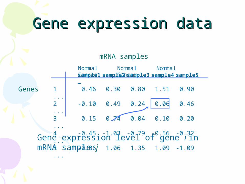
Gene expression dataGene expression data

Genes

mRNA samples

Gene expression level of gene i in mRNA sample j

sample1 sample2 sample3 sample4 sample5 …

1 0.46 0.30 0.80 1.51 0.90 ...2 -0.10 0.49 0.24 0.06 0.46 ...3 0.15 0.74 0.04 0.10 0.20 ...4 -0.45 -1.03 -0.79 -0.56 -0.32 ...5 -0.06 1.06 1.35 1.09 -1.09 ...

Normal Normal Normal Cancer Cancer

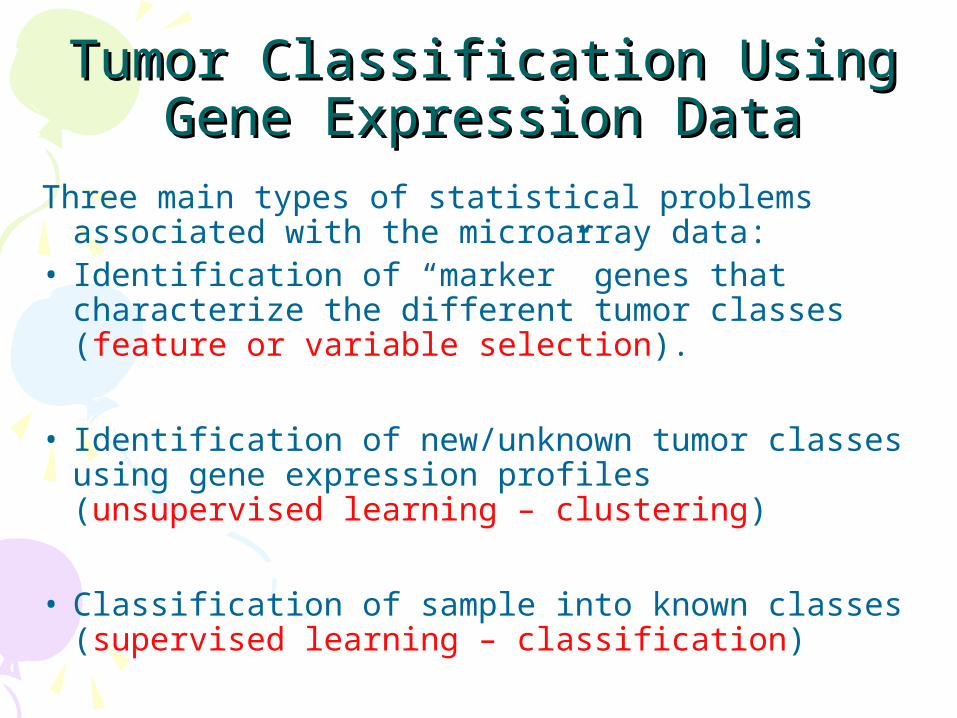
Tumor Classification Using Gene Tumor Classification Using Gene Expression DataExpression Data

Three main types of statistical problems associated with the microarray data:

• Identification of “marker” genes that characterize the different tumor classes (feature or variable selection).

• Identification of new/unknown tumor classes using gene expression profiles (unsupervised learning – clustering)

• Classification of sample into known classes (supervised learning – classification)

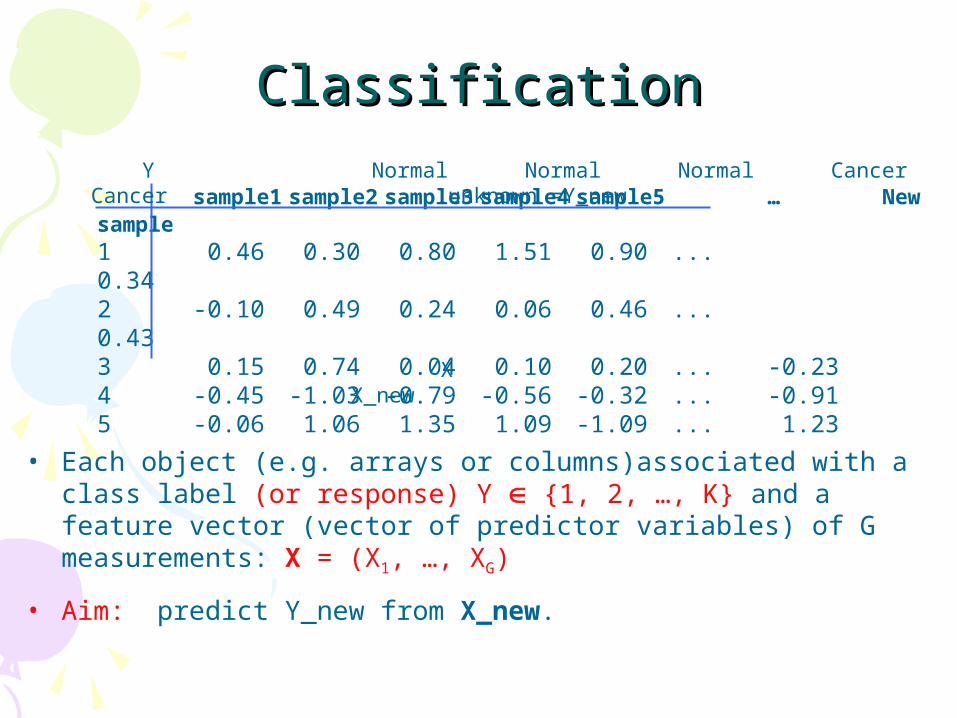
ClassificationClassification

• Each object (e.g. arrays or columns)associated with a class label (or response) Y {1, 2, …, K} and a feature vector (vector of predictor variables) of G measurements: X = (X1, …, XG)

• Aim: predict Y_new from X_new.

sample1 sample2 sample3 sample4 sample5 … New sample

1 0.46 0.30 0.80 1.51 0.90 ... 0.342 -0.10 0.49 0.24 0.06 0.46 ... 0.433 0.15 0.74 0.04 0.10 0.20 ... -0.234 -0.45 -1.03 -0.79 -0.56 -0.32 ... -0.915 -0.06 1.06 1.35 1.09 -1.09 ... 1.23

Y Normal Normal Normal Cancer Cancer unknown =Y_new

X X_new

ClassifiersClassifiers• A predictor or classifier partitions the space of gene expression profiles into

K disjoint subsets, A1, ..., AK, such that for a sample with expression profile X=(X1, ...,XG) Ak the predicted class is k.

• Classifiers are built from a learning set (LS)

L = (X1, Y1), ..., (Xn,Yn)

• Classifier C built from a learning set L: C( . ,L): X {1,2, ... ,K}

• Predicted class for observation X:

C(X,L) = k if X is in Ak

Classification MethodsClassification Methods• Fisher Linear Discriminant Analysis.• Maximum Likelihood Discriminant Rule.

– Quadratic discriminant analysis (QDA).– Linear discriminant analysis (LDA, equivalent to FLDA for K=2).– Diagnal quadratic discriminant analysis (DQDA).– Diagnal linear discriminant analysis (DLDA).

• Nearest Neighbor Classification.• Classification and Regression Tree (CART).• Aggregating & Bagging.

Fisher Linear Discriminant AnalysisFisher Linear Discriminant Analysis

-- M.Barnard. The secular variations of skull characters in four series of egyptian skulls. Annals of Eugenics, 6:352-371, 1935.

-- R.A.Fisher. The use of multiple measurements in taxonomic problems. Annals of Eugenics, 7:179-188, 1936.


• In a two-class classification problem, given n samples in a d-dimensional feature space. n1 in class 1 and n2 in class 2.

• Goal: to find a vector w, and project the n samples on the axis y=w’x, so that the projected samples are well separated.

QuickTime™ and aTIFF (LZW) decompressor

are needed to see this picture.


• The sample mean vector for the ith class is mi and the sample covariance matrix for the ith class is Si.

• The between-class scatter matrix is:

SB=(m1-m2)(m1-m2)’• The within-class scatter matrix is:

Sw= S1+S2

• The sample mean of the projected points in the ith class is:

• The variance of the projected points in the ith class is:

€

˜ m i =1

ni

w' xx∈ith class

∑ = w'mi

€

˜ S i = (w' x − w'mi)2

x∈ith class

∑ = w'Siw




€

˜ m 1

€

˜ m 2

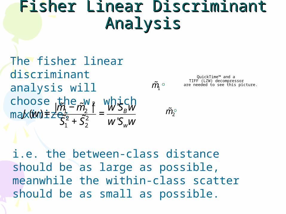
The fisher linear discriminant analysis will choose the w, which maximize:

€

J(w) =| ˜ m 1 − ˜ m 2 |2

˜ S 12 + ˜ S 2

2=

w'SB w

w'Sww

i.e. the between-class distance should be as large as possible, meanwhile the within-class scatter should be as small as possible.




For K=2, FLDA yields the same classifier as the Lear maximum likelihood discriminant rule.

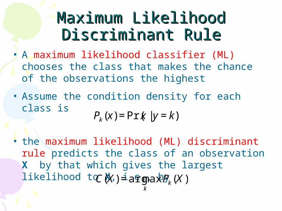
Maximum Likelihood Discriminant RuleMaximum Likelihood Discriminant Rule• A maximum likelihood classifier (ML) chooses the

class that makes the chance of the observations the highest

• Assume the condition density for each class is

• the maximum likelihood (ML) discriminant rule predicts the class of an observation X by that which gives the largest likelihood to X, i.e., by €

Pk (x) = Pr(x | y = k)

€

C(X) = argmaxk

Pk (X)

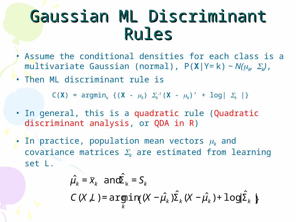
Gaussian ML Discriminant RulesGaussian ML Discriminant Rules• Assume the conditional densities for each class is a

multivariate Gaussian (normal), P(X|Y= k) ~ N(k, k),

• Then ML discriminant rule is

C(X) = argmink {(X - k) k-1

(X - k)’ + log| k |}

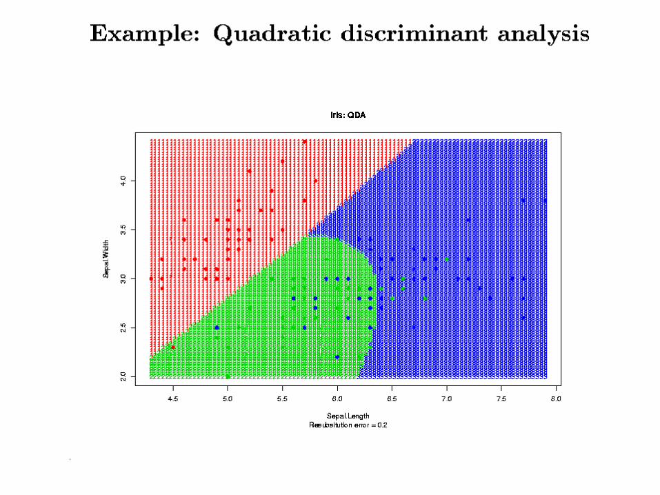
• In general, this is a quadratic rule (Quadratic discriminant analysis, or QDA in R)

• In practice, population mean vectors k and covariance matrices k are estimated from learning set L.

€

ˆ μ k = x k and ˆ Σ k = Sk

C(X,L) = argmink

(X − ˆ μ k ) ˆ Σ k (X − ˆ μ k ) + log | ˆ Σ k |{ }

Gaussian ML Discriminant RulesGaussian ML Discriminant Rules

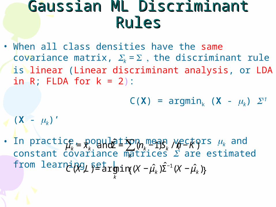
• When all class densities have the same covariance matrix, k = the discriminant rule is linear (Linear discriminant analysis, or LDA in R; FLDA for k = 2):

C(X) = argmink (X - k) -1 (X - k)’

• In practice, population mean vectors k and constant covariance matrices are estimated from learning set L.

€

ˆ μ k = x k and ˆ Σ = (nk −1)Sk

k

∑ /(n − K)

C(X,L) = argmink

(X − ˆ μ k ) ˆ Σ −1(X − ˆ μ k ){ }

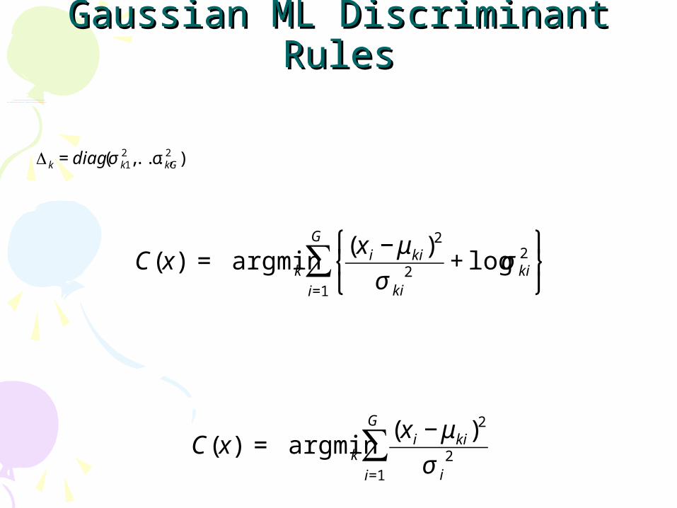
Gaussian ML Discriminant RulesGaussian ML Discriminant Rules•

When the class densities have diagonal covariance matrices,

, the discriminant rule is given by addit ive quadratic contribut ions from each variable (Diagonal quadratic discriminant analysis, or DQDA)

• When all class densities have the same diagonal covariance matrix =diag(12… G

2 ), the discriminant rule is again linear (Diagonal linear discriminant analysis, or DLDA in R)

€

C(x) = argmink

(x i − μ ki)2

σ i2

i=1

G

∑

€

k = diag(σ k12 ,...,σ kG

2 )

€

C(x) = argmink

(x i − μ ki)2

σ ki2 + logσ ki

2 ⎧ ⎨ ⎩

⎫ ⎬ ⎭i=1

G

∑

Application of ML discriminant Application of ML discriminant RuleRule

• Weighted gene voting method. (Golub et al. 1999)– One of the first application of a ML discriminant rule to gene

expression data. – This methods turns out to be a minor variant of the sample

Diagonal Linear Discriminant rule.

– Golub TR, Slonim DK, Tamayo P, Huard C, Gaasenbeek M, Mesirov JP,Coller H, Loh ML, Downing JR, Caligiuri MA, Bloomfield CD, Lander ES. (1999).Molecular classification of cancer: class discovery and class prediction bygene expression monitoring. Science. Oct 15;286(5439):531 - 537.

Example: Weighted gene voting methodExample: Weighted gene voting method

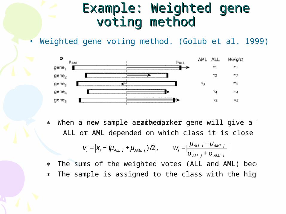
• Weighted gene voting method. (Golub et al. 1999)

€

∗ When a new sample arrived, each marker gene will give a vote for either

ALL or AML depended on which class it is close to.

v i = x i − (μALL,i + μAML,i) /2, wi =|μALL,i − μAML,i

σ ALL ,i + σ AML,i

|

∗ The sums of the weighted votes (ALL and AML) become the total votes.

∗ The sample is assigned to the class with the higher total vote,

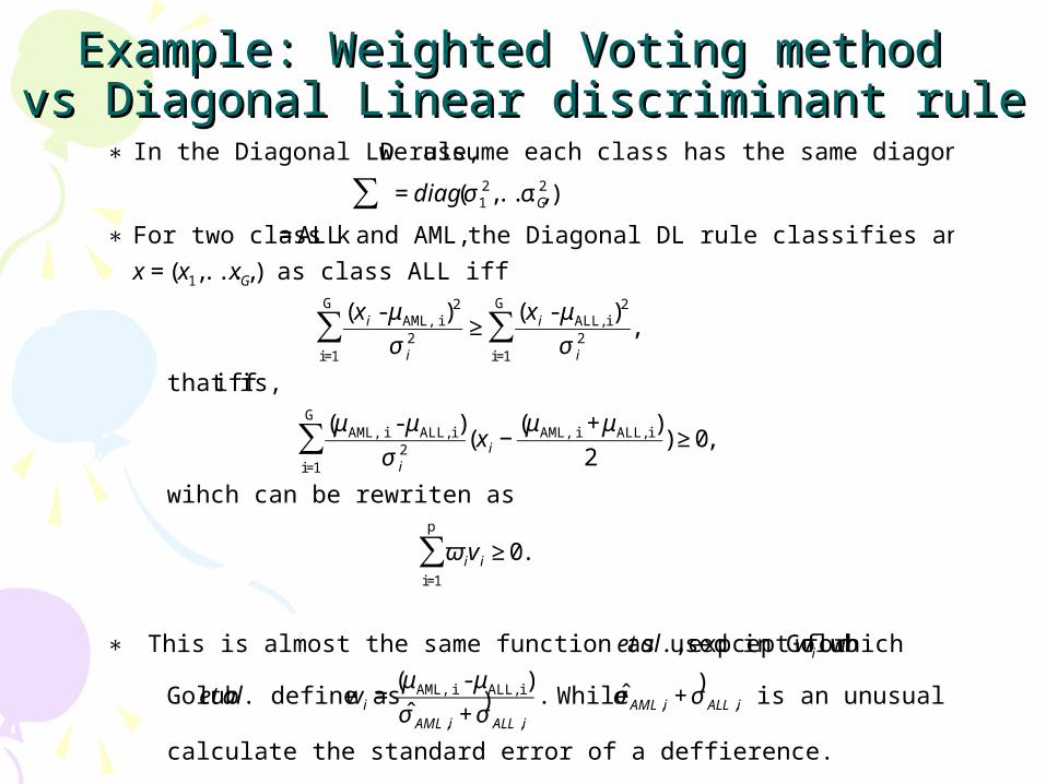
Example: Weighted Voting method Example: Weighted Voting method vs Diagonal Linear discriminant rulevs Diagonal Linear discriminant rule

€

∗ In the Diagonal LD rule, we assume each class has the same diagonal covariance.

∑ = diag(σ 12,...,σ G

2 )

∗ For two class k = ALL and AML, the Diagonal DL rule classifies an observation

x = (x1,...,xG ) as class ALL iff

(x i - μAML,i)

2

σ i2

i=1

G

∑ ≥(x i - μALL,i)

2

σ i2

i=1

G

∑ ,

that is, iff

(μAML,i - μALL,i)

σ i2

i=1

G

∑ (x i −(μAML,i +μALL,i)

2) ≥ 0,

wihch can be rewriten as

ϖ i

i=1

p

∑ v i ≥ 0.

∗ This is almost the same function as used in Golub et al., expcept for wi which

Golub et al. define as wi =(μAML,i - μALL,i)ˆ σ AML,i +

) σ ALL ,i

. While ˆ σ AML,i +) σ ALL,i is an unusual way to

calculate the standard error of a deffierence.

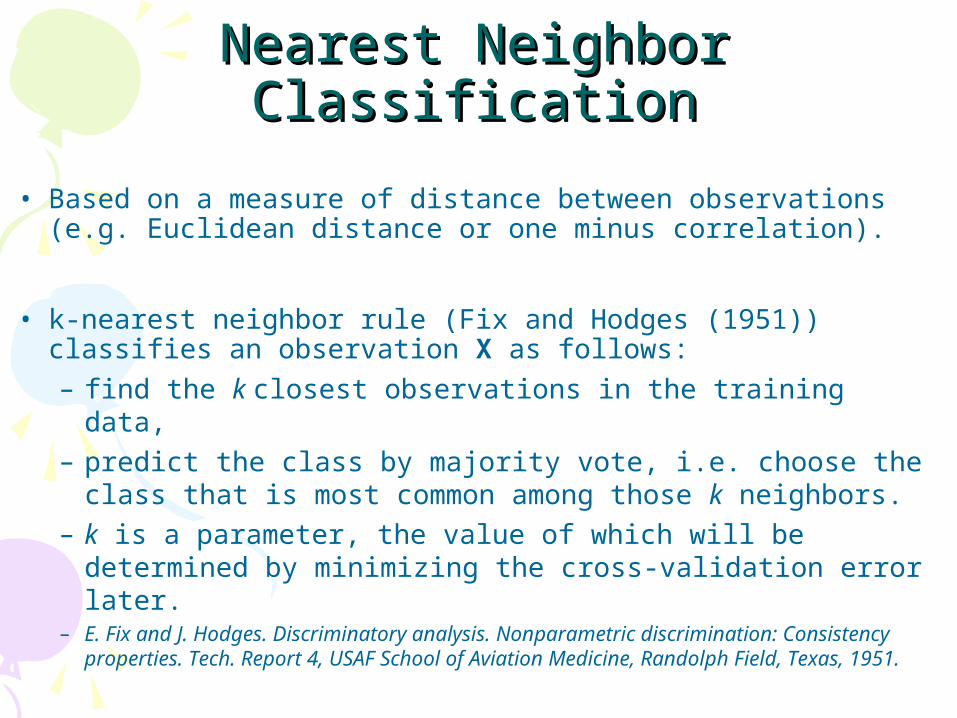
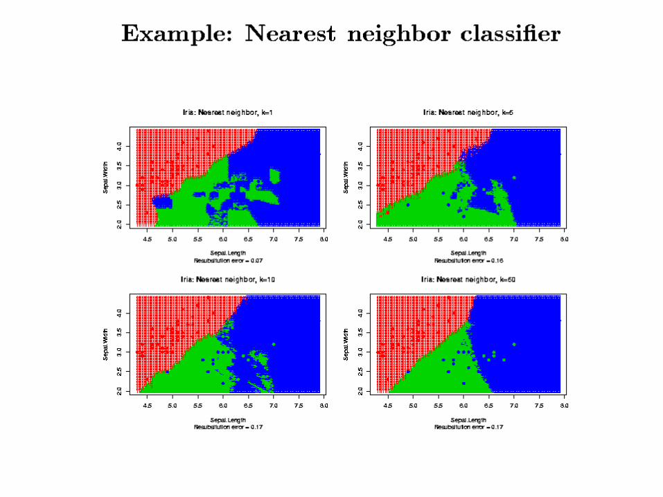
Nearest Neighbor ClassificationNearest Neighbor Classification

• Based on a measure of distance between observations (e.g. Euclidean distance or one minus correlation).

• k-nearest neighbor rule (Fix and Hodges (1951)) classifies an observation X as follows:

– find the k closest observations in the training data,– predict the class by majority vote, i.e. choose the class that

is most common among those k neighbors.– k is a parameter, the value of which will be determined by

minimizing the cross-validation error later.– E. Fix and J. Hodges. Discriminatory analysis. Nonparametric

discrimination: Consistency properties. Tech. Report 4, USAF School of Aviation Medicine, Randolph Field, Texas, 1951.

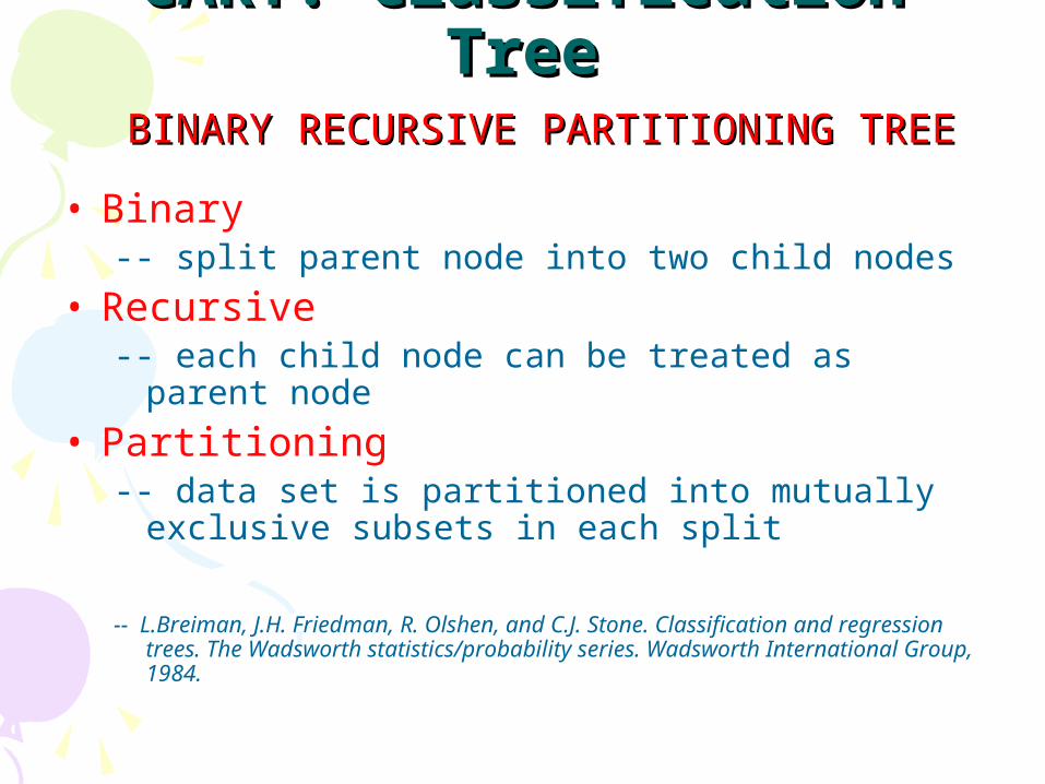
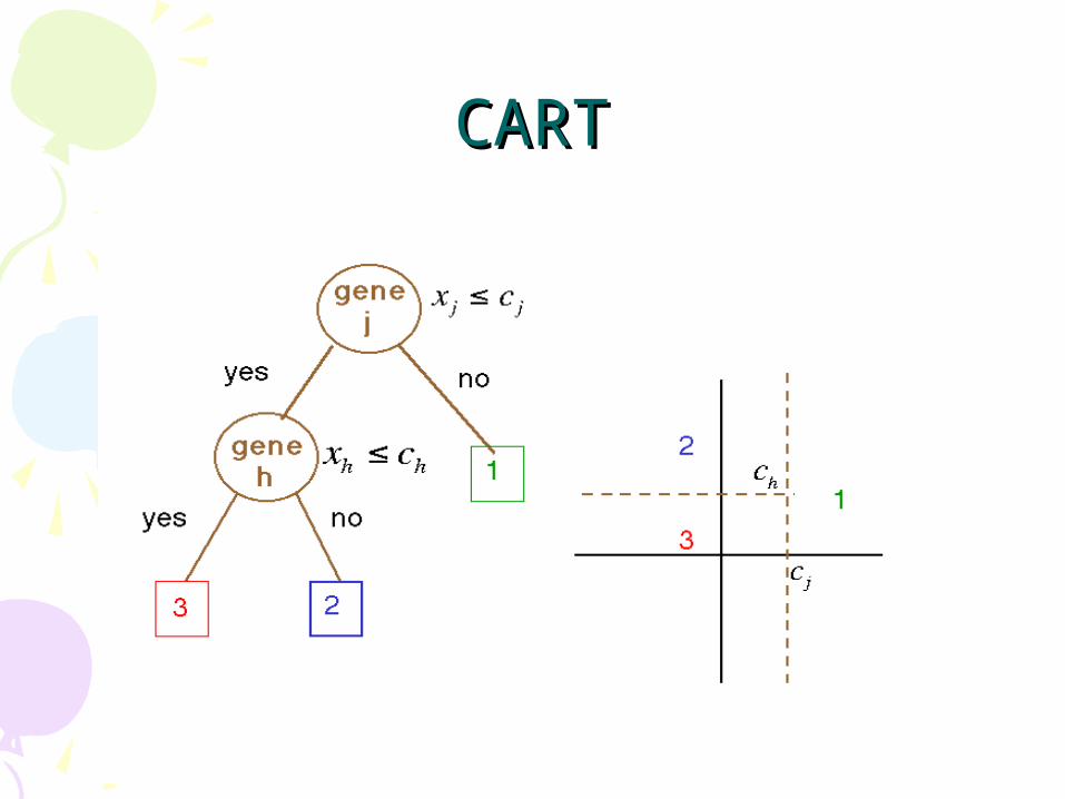
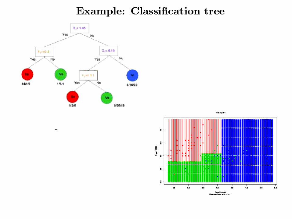
CART: Classification TreeCART: Classification Tree BINARY RECURSIVE PARTITIONING TREEBINARY RECURSIVE PARTITIONING TREE

• Binary-- split parent node into two child nodes

• Recursive -- each child node can be treated as parent node

• Partitioning-- data set is partitioned into mutually exclusive

subsets in each split

-- L.Breiman, J.H. Friedman, R. Olshen, and C.J. Stone. Classification and regression trees. The Wadsworth statistics/probability series. Wadsworth International Group, 1984.

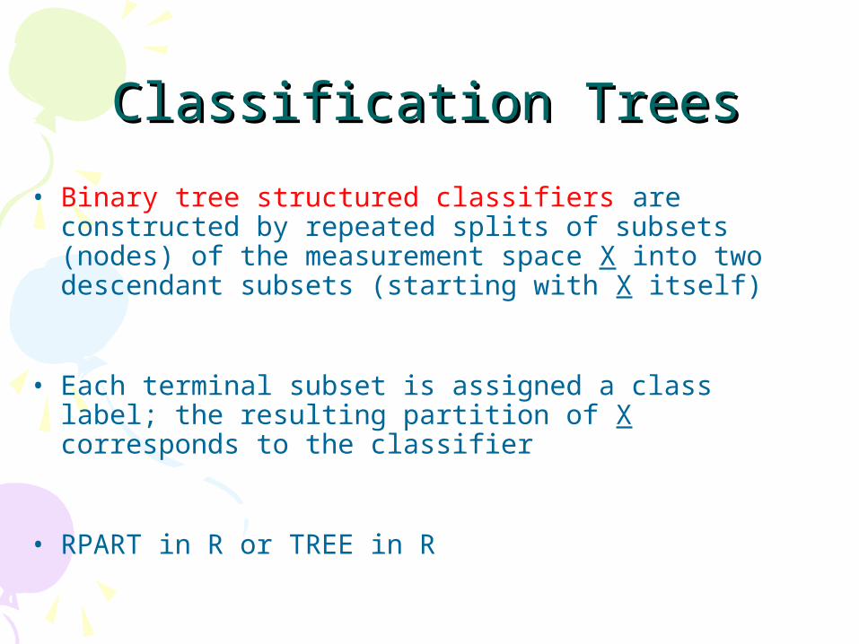
Classification TreesClassification Trees

• Binary tree structured classifiers are constructed by repeated splits of subsets (nodes) of the measurement space X into two descendant subsets (starting with X itself)

• Each terminal subset is assigned a class label; the resulting partition of X corresponds to the classifier

• RPART in R or TREE in R

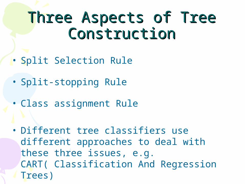
Three Aspects of Tree Three Aspects of Tree ConstructionConstruction

• Split Selection Rule

• Split-stopping Rule

• Class assignment Rule

• Different tree classifiers use different approaches to deal with these three issues, e.g. CART( Classification And Regression Trees)

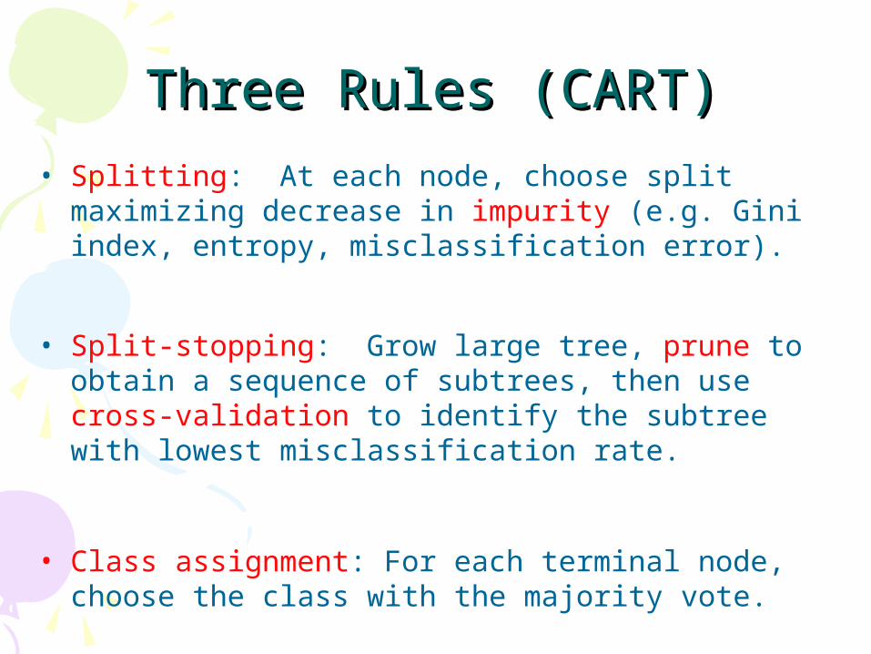
Three Rules (CART)Three Rules (CART)

• Splitting: At each node, choose split maximizing decrease in impurity (e.g. Gini index, entropy, misclassification error).

• Split-stopping: Grow large tree, prune to obtain a sequence of subtrees, then use cross-validation to identify the subtree with lowest misclassification rate.

• Class assignment: For each terminal node, choose the class with the majority vote.

CARTCART

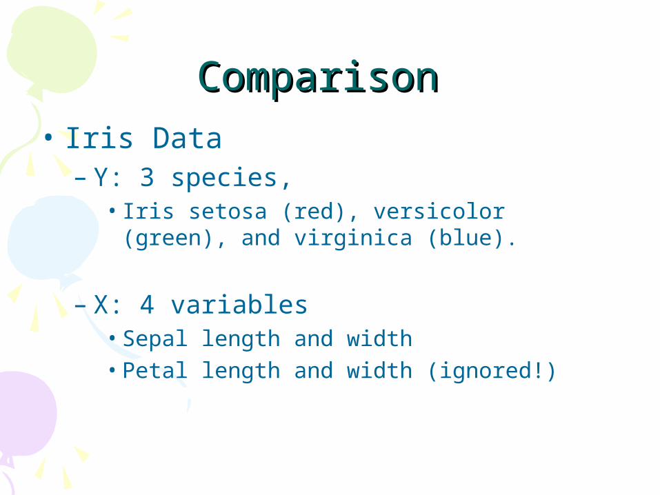
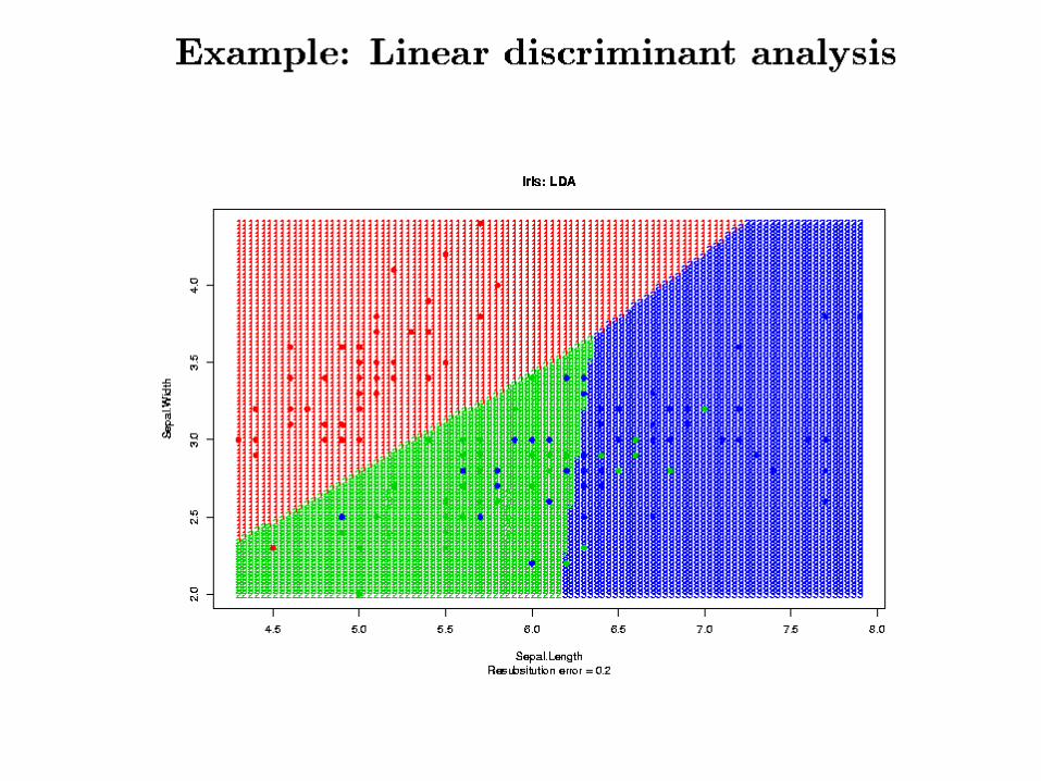
Comparison Comparison

• Iris Data– Y: 3 species,

• Iris setosa (red), versicolor (green), and virginica (blue).

– X: 4 variables• Sepal length and width • Petal length and width (ignored!)

Other Classifiers Include…Other Classifiers Include…

• Support vector machines (SVMs)

• Neural networks

• HUNDREDS more…

• The Best Reference: Google

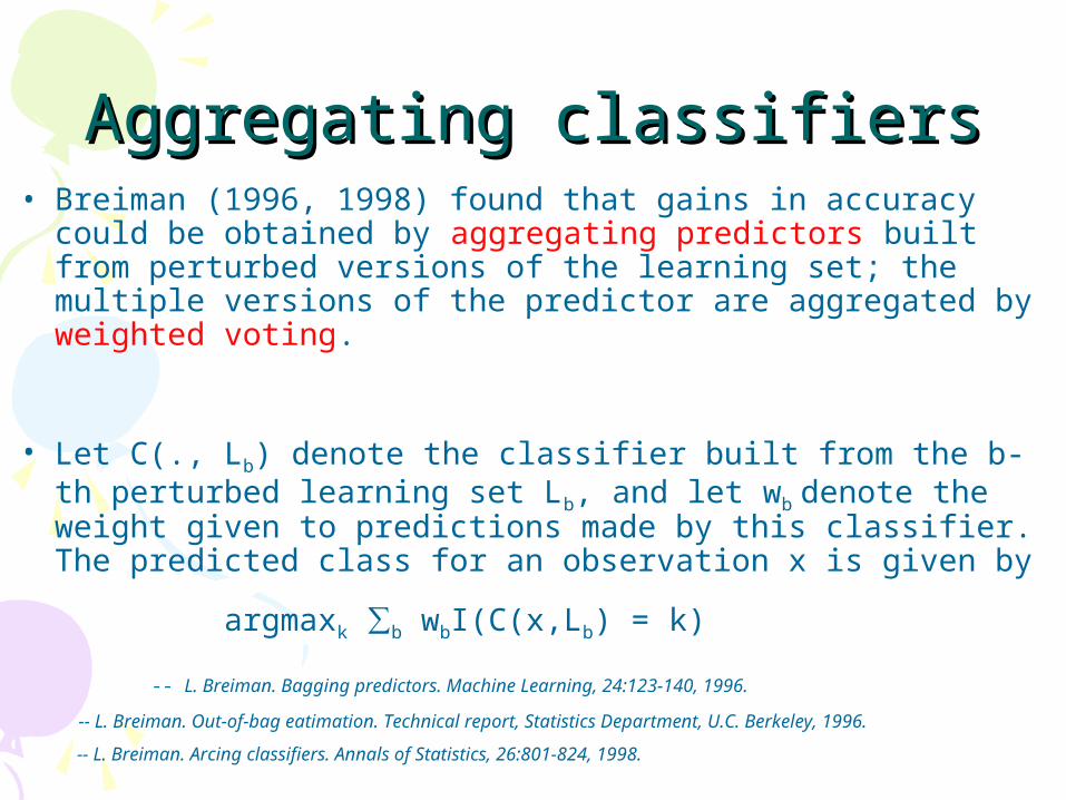
Aggregating classifiersAggregating classifiers• Breiman (1996, 1998) found that gains in accuracy could be

obtained by aggregating predictors built from perturbed versions of the learning set; the multiple versions of the predictor are aggregated by weighted voting.

• Let C(., Lb) denote the classifier built from the b-th perturbed learning set Lb, and let wb denote the weight given to predictions made by this classifier. The predicted class for an observation x is given by

argmaxk ∑b wbI(C(x,Lb) = k)

-- L. Breiman. Bagging predictors. Machine Learning, 24:123-140, 1996.

-- L. Breiman. Out-of-bag eatimation. Technical report, Statistics Department, U.C. Berkeley, 1996.

-- L. Breiman. Arcing classifiers. Annals of Statistics, 26:801-824, 1998.

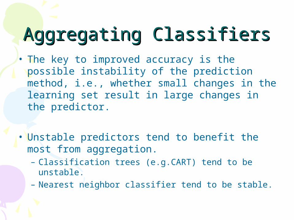
Aggregating ClassifiersAggregating Classifiers• The key to improved accuracy is the possible

instability of the prediction method, i.e., whether small changes in the learning set result in large changes in the predictor.

• Unstable predictors tend to benefit the most from aggregation.– Classification trees (e.g.CART) tend to be unstable.– Nearest neighbor classifier tend to be stable.

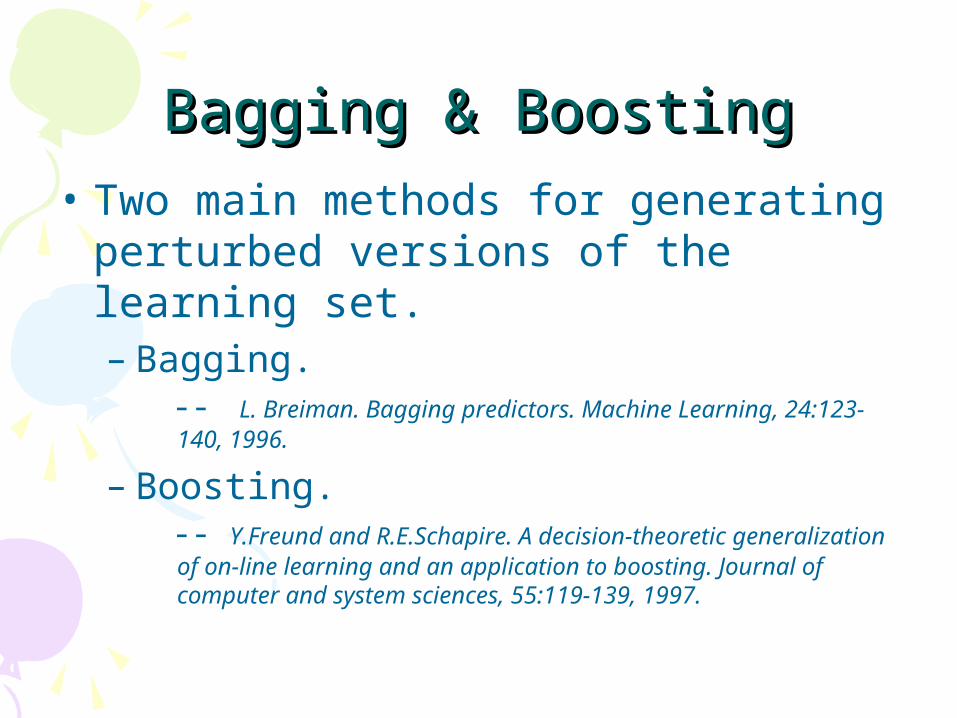
Bagging & BoostingBagging & Boosting

• Two main methods for generating perturbed versions of the learning set.– Bagging.

-- L. Breiman. Bagging predictors. Machine Learning, 24:123-140, 1996.

– Boosting. -- Y.Freund and R.E.Schapire. A decision-theoretic generalization of

on-line learning and an application to boosting. Journal of computer and system sciences, 55:119-139, 1997.

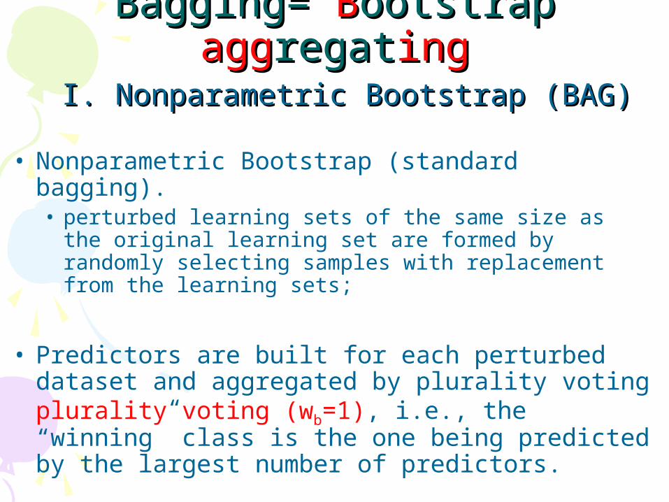
Bagging= Bagging= BBootstrap ootstrap aggaggregatregatinging I. Nonparametric Bootstrap (BAG)I. Nonparametric Bootstrap (BAG)

• Nonparametric Bootstrap (standard bagging).• perturbed learning sets of the same size as the original

learning set are formed by randomly selecting samples with replacement from the learning sets;

• Predictors are built for each perturbed dataset and aggregated by plurality voting plurality voting (wb=1), i.e., the “winning” class is the one being predicted by the largest number of predictors.

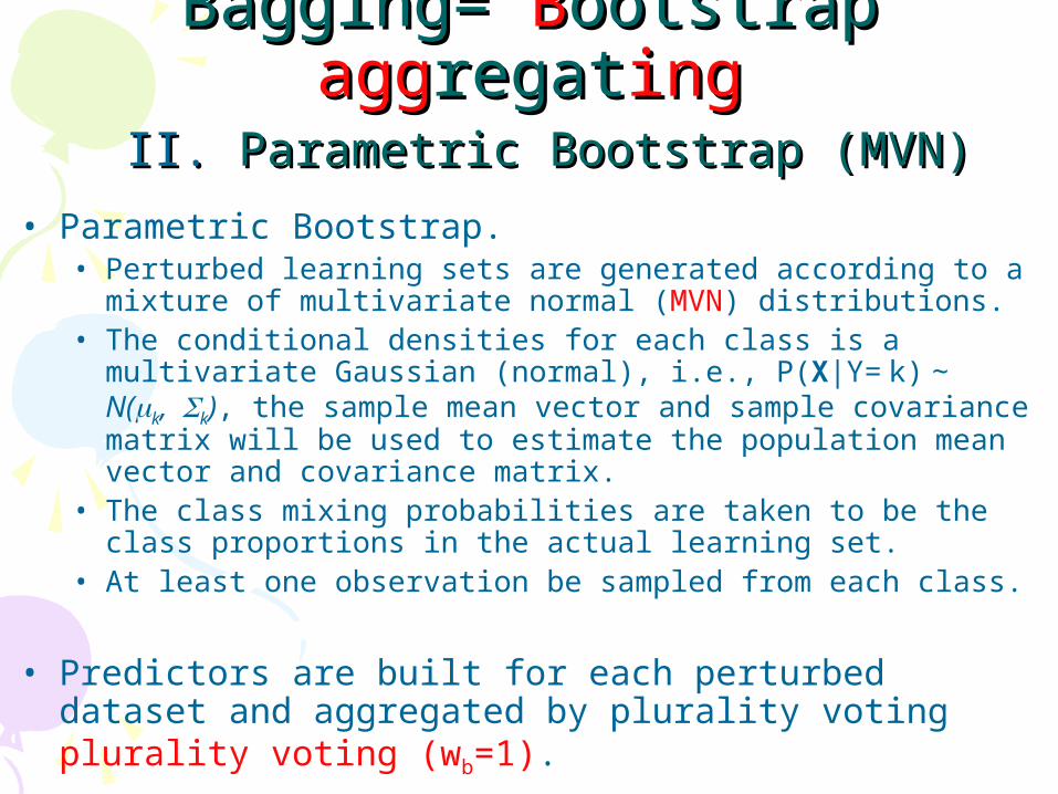
Bagging= Bagging= BBootstrap ootstrap aggaggregatregatinging II. II. Parametric Bootstrap (MVN)Parametric Bootstrap (MVN)

• Parametric Bootstrap.• Perturbed learning sets are generated according to a mixture of

multivariate normal (MVN) distributions.• The conditional densities for each class is a multivariate Gaussian

(normal), i.e., P(X|Y= k) ~ N(k, k), the sample mean vector and sample covariance matrix will be used to estimate the population mean vector and covariance matrix.

• The class mixing probabilities are taken to be the class proportions in the actual learning set.

• At least one observation be sampled from each class.

• Predictors are built for each perturbed dataset and aggregated by plurality voting plurality voting (wb=1).

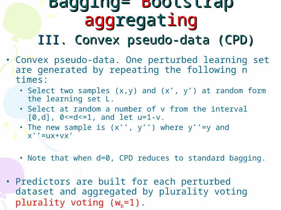
Bagging= Bagging= BBootstrap ootstrap aggaggregatregatinging III. III. Convex pseudo-data (CPD)Convex pseudo-data (CPD)

• Convex pseudo-data. One perturbed learning set are generated by repeating the following n times:• Select two samples (x,y) and (x’, y’) at random form the learning set L.• Select at random a number of v from the interval [0,d], 0<=d<=1, and

let u=1-v.• The new sample is (x’’, y’’) where y’’=y and x’’=ux+vx’

• Note that when d=0, CPD reduces to standard bagging.

• Predictors are built for each perturbed dataset and aggregated by plurality voting plurality voting (wb=1).

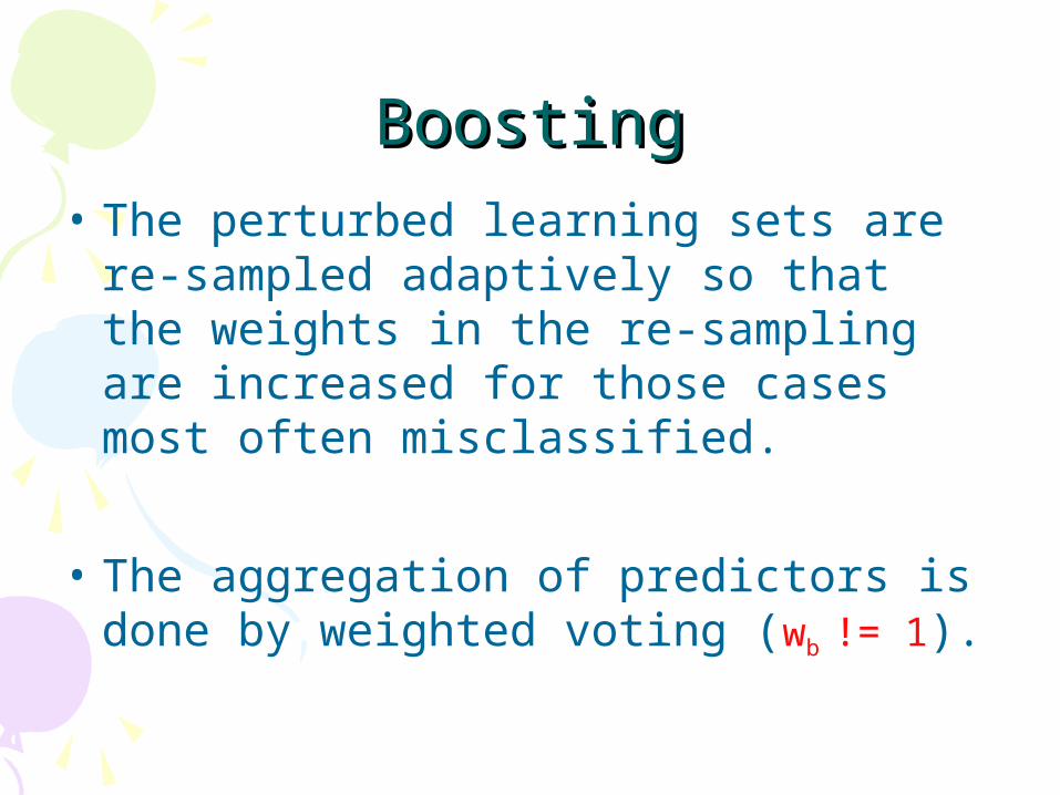
BoostingBoosting

• The perturbed learning sets are re-sampled adaptively so that the weights in the re-sampling are increased for those cases most often misclassified.

• The aggregation of predictors is done by weighted voting (wb != 1).

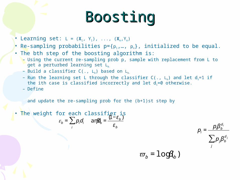
BoostingBoosting• Learning set: L = (X1, Y1), ..., (Xn,Yn)

• Re-sampling probabilities p={p1,…, pn}, initialized to be equal.• The bth step of the boosting algorithm is:

– Using the current re-sampling prob p, sample with replacement from L to get a perturbed learning set Lb.

– Build a classifier C(., Lb) based on Lb.

– Run the learning set L through the classifier C(., Lb) and let di=1 if the ith case is classified incorrectly and let di=0 otherwise.

– Define

and update the re-sampling prob for the (b+1)st step by

• The weight for each classifier is

€

εb = pidi

i

∑ and β b =(1−εb )

εb

€

pi =piβ b

d i

p jβ bd j

j

∑

€

ϖb = log(β b )

Comparison of classifiersComparison of classifiers• Dudoit, Fridlyand, Speed (JASA, 2002)

• FLDA (Fisher Linear Discriminant Analysis)

• DLDA (Diagonal Linear Discriminant Analysis)

• DQDA (Diagonal Quantic Discriminant Analysis)

• NN (Nearest Neighbour)

• CART (Classification and Regression Tree)

• Bagging and boosting • Bagging (Non-parametric Bootstrap )

• CPD (Convex Pseudo Data)

• MVN (Parametric Bootstrap)

• Boosting

-- Dudoit, Fridlyand, Speed: “Comparison of discrimination methods for the classification of tumors using gene expression data”, JASA, 2002

Comparison study datasetsComparison study datasets• Leukemia – Golub et al. (1999)

n = 72 samples, G = 3,571 genes

3 classes (B-cell ALL, T-cell ALL, AML)

• Lymphoma – Alizadeh et al. (2000)n = 81 samples, G = 4,682 genes

3 classes (B-CLL, FL, DLBCL)

• NCI 60 – Ross et al. (2000)N = 64 samples, p = 5,244 genes

8 classes

ProcedureProcedure• For each run (total 150 runs):

– 2/3 of sample randomly selected as learning set (LS), rest 1/3 as testing set (TS).

– The top p genes with the largest BSS/WSS are selected using the learning set.

• p=50 for lymphoma dataset.• p=40 for leukemia dataset.• p=30 for NCI 60 dataset.

– Predictors are constructed and error rated are obtained by applying the predictors to the testing set.

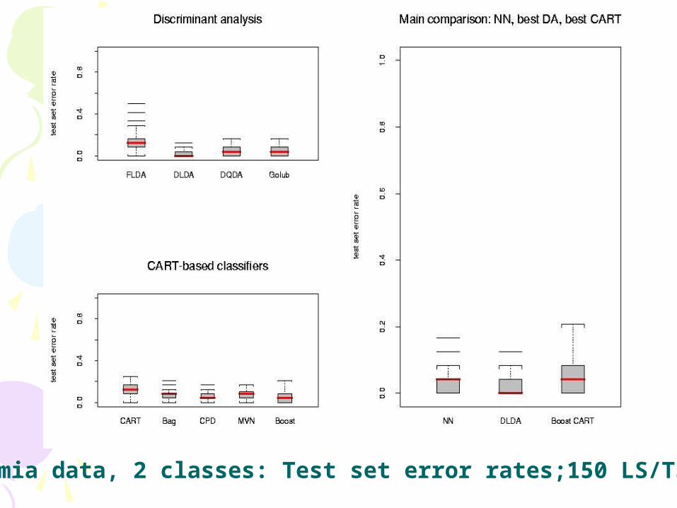
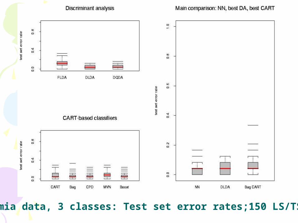
Leukemia data, 2 classes: Test set error rates;150 LS/TS runs

Leukemia data, 3 classes: Test set error rates;150 LS/TS runs

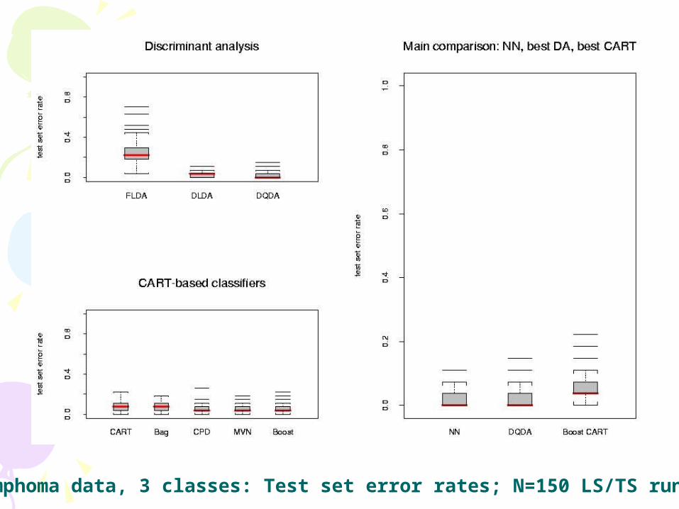
Lymphoma data, 3 classes: Test set error rates; N=150 LS/TS runs

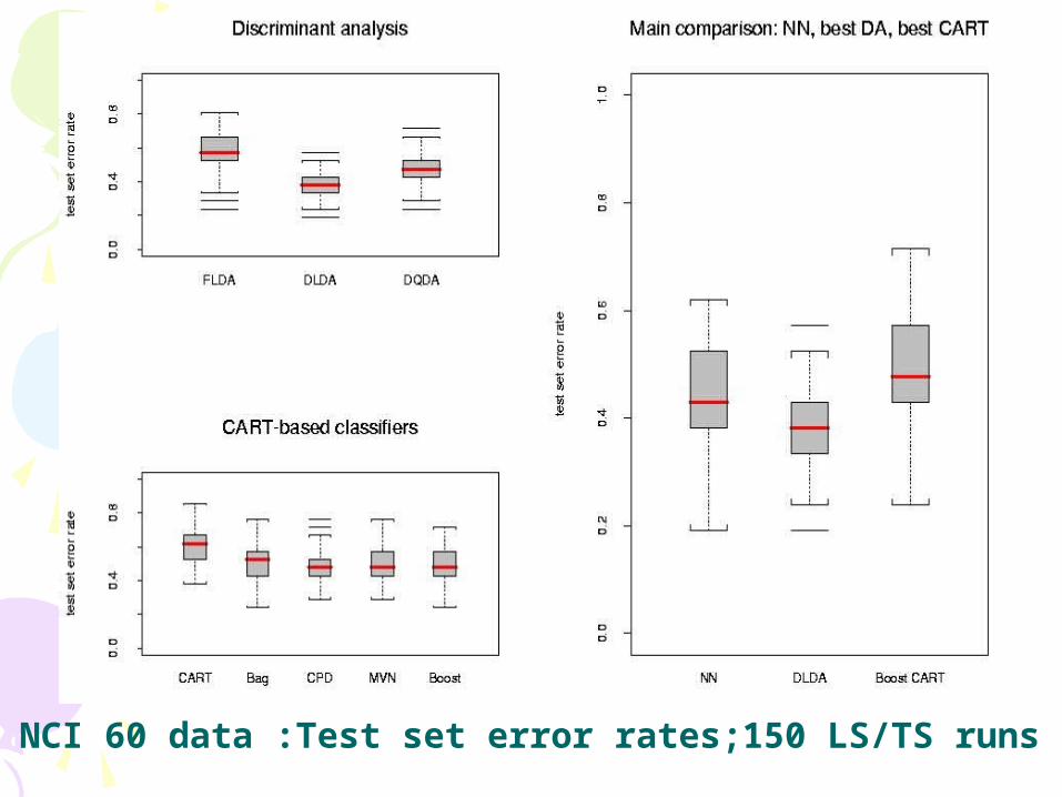
NCI 60 data :Test set error rates;150 LS/TS runs

ResultsResults• In the main comparison of Dudoit et al, NN

and DLDA had the smallest error rates, FLDA had the highest

• For the lymphoma and leukemia datasets, increasing the number of genes to G=200 didn't greatly affect the performance of the various classifiers; there was an improvement for the NCI 60 dataset.

• More careful selection of a small number of genes (10) improved the performance of FLDA dramatically

Comparison study – Discussion (I)Comparison study – Discussion (I)

• “Diagonal” LDA: ignoring correlation between genes helped here. Unlike classification trees and nearest neighbors, LDA is unable to take into account gene interactions

• Although nearest neighbors are simple and intuitive classifiers, their main limitation is that they give very little insight into mechanisms underlying the class distinctions

Comparison study – Discussion (II)Comparison study – Discussion (II)

• Variable selection: A crude criterion such as BSS/WSS may not identify the genes that discriminate between all the classes and may not reveal interactions between genes

• With larger training sets, expect improvement in performance of aggregated classifiers

AcknowledgementsAcknowledgements

• Some of slides adapted form http://statwww.epfl.ch/davison/teaching/Microarrays/ by Darlene Goldstein

Thank you!

Documents

Xuelian Wei Department of Statistics Most of Slides Adapted from by Darlene Goldstein Classification