Embed Size (px)
Citation preview
Zigzag Learning for Weakly Supervised Object Detection
Xiaopeng Zhang1 Jiashi Feng1 Hongkai Xiong2 Qi Tian3
1 National University of Singapore 2 Shanghai Jiao Tong University 3 University of Texas at San Antonio
elezxi,[email protected] [email protected] [email protected]
Abstract
This paper addresses weakly supervised object detection
with only image-level supervision at training stage. Previ-
ous approaches train detection models with entire images
all at once, making the models prone to being trapped in
sub-optimums due to the introduced false positive examples.
Unlike them, we propose a zigzag learning strategy to si-
multaneously discover reliable object instances and prevent
the model from overfitting initial seeds. Towards this goal,
we first develop a criterion named mean Energy Accumula-
tion Scores (mEAS) to automatically measure and rank lo-
calization difficulty of an image containing the target object,
and accordingly learn the detector progressively by feeding
examples with increasing difficulty. In this way, the mod-
el can be well prepared by training on easy examples for
learning from more difficult ones and thus gain a stronger
detection ability more efficiently. Furthermore, we intro-
duce a novel masking regularization strategy over the high
level convolutional feature maps to avoid overfitting initial
samples. These two modules formulate a zigzag learning
process, where progressive learning endeavors to discov-
er reliable object instances, and masking regularization in-
creases the difficulty of finding object instances properly.
We achieve 47.6% mAP on PASCAL VOC 2007, surpassing
the state-of-the-arts by a large margin.
1. Introduction
Current state-of-the-art object detection performance has
been achieved with a fully supervised paradigm. Howev-
er, it requires a large quantity of high-quality object-level
annotations (i.e., object bounding boxes) at training stages
[1], [2], [3], which are very costly to collect. Fortunate-
ly, the prevalence of image tags allows search engines to
quickly provide a set of images related to the target catego-
ry [4], [5], making image-level annotations much easier to
acquire. Hence it is more appealing to learn detection mod-
els from such weakly labeled images. In this paper, we fo-
cus on object detection under a weakly supervised paradig-
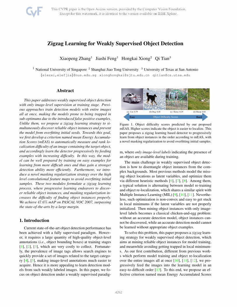
Object Difficulty ScoresEasy Hard
(d) Sheep: 0.02(b) Dog: 0.44 (c) Horse: 0.29(a) Car: 0.79
Figure 1. Object difficulty scores predicted by our proposed
mEAS. Higher scores indicate the object is easier to localize. This
paper proposes a zigzag learning based detector to progressively
learn from object instances in the order according to mEAS, with
a novel masking regularization to avoid overfitting initial samples.
m, where only image-level labels indicating the presence of
an object are available during training.
The main challenge in weakly supervised object detec-
tion is how to disentangle object instances from the com-
plex backgrounds. Most previous methods model the miss-
ing object locations as latent variables, and optimize them
via different heuristic methods [6], [7], [8]. Among them,
a typical solution is alternating between model re-training
and object re-localization, which shares a similar spirit with
Multiple Instance Learning (MIL) [9], [10], [11]. Neverthe-
less, such optimization is non-convex and easy to get stuck
in local minimums if the latent variables are not properly
initialized. Then mining object instances with only image-
level labels becomes a classical chicken-and-egg problem:
without an accurate detection model, object instances can-
not be discovered, while an accurate detection model cannot
be learned without appropriate object examples.
To solve this problem, this paper proposes a zigzag learn-
ing strategy for weakly supervised object detection, which
aims at mining reliable object instances for model training,
and meanwhile avoiding getting trapped in local minimum-
s. As our first contribution, different from previous work-
s which perform model training and object re-localization
over the entire images all at once [10], [11], [12], we pro-
gressively feed the images into the learning model in an
easy-to-difficult order [13]. To this end, we propose an ef-
fective criterion named mean Energy Accumulated Scores
4262
(mEAS) to automatically measure the difficulty of an image
containing the target object, and progressively add samples
during model training. As shown in Fig. 1, car and dog are
simpler to localize while horse and sheep are more difficult.
Intuitively, ignoring this discrepancy of object difficulty in
localization would inevitably include many poorly localized
samples, which deteriorates the trained model. On the other
hand, processing easier images in the initial stages leads to
better detection models, which in turn increases the proba-
bility of successfully localizing objects in difficult images.
Due to lack of object annotations, the mined object in-
stances inevitably include false positive samples. Current
approaches [10], [11] simply treat these pseudo annotations
as ground truth, which is suboptimal and easy to overfit the
initial seeds. This is especially true for a deep network due
to its high fitting capacity. As our second contribution, we
design a novel masking strategy over the last convolution-
al feature maps, which randomly erases the discriminative
regions during training. It prevents the model from concen-
trating on part details at earlier training, and induces the net-
work to focus more on those less discriminative parts at cur-
rent training. In this way, the model is able to discover more
integrated objects as desired. Another advantage is that the
proposed masking operation introduces many random oc-
cluded samples, which can be treated as data augmentation
and enhances the generalization ability of the model.
Integrating the progressive learning and masking regu-
larization formulates a zigzag learning process. The pro-
gressive learning endeavours to discover reliable object in-
stances in an easy-to-difficult order, while the masking strat-
egy increases the difficulty in a way favorable of object min-
ing via introducing many random occluded samples. These
two adversarial modules boost each other, and benefit both
object instance mining and reducing model overfitting risks.
The effectiveness of zigzag learning has been validated ex-
perimentally. On benchmark dataset PASCAL VOC 2007,
we achieve an accuracy of 47.6% under weakly supervised
paradigm, which surpasses the-state-of-the-arts by a large
margin. To sum up, we make following contributions.
• We propose a new and effective criterion named mean
Energy Accumulated Scores (mEAS) to automatically mea-
sure the difficulty of an image w.r.t. localizing a specific
object. Based on mEAS, we train detection models via an
easy-to-hard strategy. This kind of progressive learning is
beneficial to finding reliable object instances especially for
the difficult images.
• We introduce a feature masking strategy during an end-
to-end model learning, which not only forces the network to
focus on less discriminative details during training, but also
avoids model overfitting via introducing random occluded
positive instances. Integrating these two components gives
a novel zigzag learning method and achieves state-of-the-art
performance for weakly supervised object detection.
2. Related Works
Our method is related with two fields: 1) image difficulty
evaluation; 2) weakly supervised detection.
Evaluating image difficulty. Little literature has been
devoted to evaluating the difficulty of an image. A prelim-
inary work in [14] estimates the image difficulty via ana-
lyzing some low-level cues such as edges, segments, and
objectness scores. Similarly, [15] assumes that image d-
ifficulty is most related with the object size, and builds a
regression model to estimate the object size in an image.
However, it needs extra object size annotations for training
the regressor. In contrast, we propose an easy-to-compute
criterion named mean Accumulated Energy Scores (mEAS)
to automatically measure the difficulty of an image. The ad-
vantage is that the criterion is based on the network itself,
and free of human interpretation.
Weakly supervised detection. It is intuitive to mine
object instances from weakly labeled images [7], [8], [10],
and follow the pipeline of fully supervised detection based
on the mined objects. Our proposed method is most re-
lated with [9], [10], [11], which try to obtain reliable ob-
ject instances via an iterative updating strategy. However,
these methods either detach the feature extraction and mod-
el training into separate steps [9], [10], or simply utilize
the high representation ability of CNN without consider-
ing model overfitting [11], which results in limited perfor-
mance. Comparatively, we integrate model training and ob-
ject mining into a unified framework, and propose a zigzag
learning strategy to improve the generalization ability of the
model. These modifications enable us to achieve superior
detection accuracy under the weakly supervised paradigm.
Our method is also related with [16], [17]. Oquab et
al. [16] proposed a weakly supervised object localization
method by explicitly searching over candidate object lo-
cations at different scales during training. However, their
localization result is limited since it only returns a center
point for an object, not the tight bounding box. Bilen [17]
et al. proposed to model image-level loss as the accumu-
lated scores over regions and performed detection based on
the region scores. Nevertheless, this network is modeled as
classification loss, which makes the detection model easily
focus on object parts rather than the whole objects.
3. Method
In this section, we elaborate on the proposed zigza-
g learning based weakly supervised detection model. It-
s overall architecture consists of three modules, as shown
in Fig. 2. The first module estimates image difficulty au-
tomatically via a backbone network [18] trained with only
image-level labels. The second module progressively adds
samples to network training in an ascending order based on
image difficulty. Third, we incorporate convolutional fea-
4263
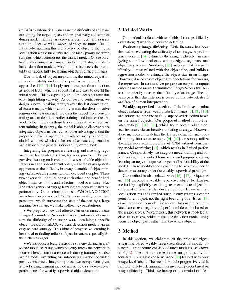
Easy
Hard
RoI
pooling
Conv5 maps
Edge boxes
Random
masking
Masked maps Fc layers
Initialize
Relocalize
Retrain
Relocalize
Retrain
Relocalize
Weighted
classif. loss
Weighted
bbox reg. loss
Figure 2. Architecture of our proposed zigzag detection network. We first estimate the image difficulty with mean Accumulated Energy
Scores (mEAS), organizing training images in an easy-to-difficult order. Then we introduce a masking strategy over the last convolutional
feature maps of fast RCNN framework, which enhances the generalization ability of the model.
ture masking into model training to regularize the high re-
sponsive patches during previous training and enhance the
generalization ability of the model. In the following, we
discuss these modules in details.
3.1. Estimating Image Difficulty
Images differ in their difficulty for localization, which
comes from factors such as object size, background clut-
ter, number of objects, and partial occlusion. For subjective
evaluation, image difficulty can be quantified as the time
needed by a human to determine the actual position of a
given class [14]. However, this brings about extra human
efforts. In this subsection, we evaluate the image difficulty
via diagnosing its localization outputs.
WSDDN framework. Our method needs a pretrained
model to diagnose the localization outputs of an image.
Without loss of generality, we use WSDDN [17] as the
baseline network, for its effectiveness and implementa-
tion convenience. WSDDN explicitly models image-level
classification loss via aggregating region proposal scores.
Specifically, given an image x with region proposals R, and
image level labels y ∈ 1,−1C , where yc = 1 (yc =−1)
indicates the presence (absence) of an object class c. De-
note the outputs of fc8C and fc8R layer as φ(x, fc8C) and
φ(x, fc8R), respectively, which are with size C×|R|. Here,
C represents the number of categories and |R| denotes the
number of regions. The score of region r corresponding to
class c is the dot product of the two fully connected layers
φ(x, fc8C) and φ(x, fc8R), normalized at different dimen-
sions:
xcr =eφ
cr(x,fc8C)
∑C
i=1 eφir(x,fc8C)
. ∗eφ
cr(x,fc8R)
∑|R|j=1 e
φcj(x,fc8R). (1)
Based on the region-level score xcr, the probability output
y w.r.t. category c at image-level is defined as the sum of a
series of region-level scores:
φc(x,wcls) =
|R|∑
j=1
xcj , (2)
where wcls denotes the non-linear mapping from input
x to classification stream output. This network is back-
propagated via a binary log image-level loss, denoted as
Lcls(x, y) =
C∑
i=1
log(yi(φi(x,wcls)− 1/2) + 1/2), (3)
and is able to automatically localize the regions which con-
tribute most to the image level scores.
Mean Energy Accumulated Scores (mEAS). Benefit-
ing from the competitive mechanism, WSDDN is able to
pick out the most discriminative details for classification.
These details sometimes fortunately correspond to the w-
hole object, but in most cases only focus on object parts.
We observe that the successfully localized objects usually
appear in relatively simple, uniform background with only
a few objects in the image. In order to pick out images that
WSDDN localizes successfully, we propose an effective cri-
terion named mean Energy Accumulated Scores (mEAS) to
quantify the localization difficulty of each image.
If the target object is easy to localize, the regions that
contribute most to the classification scores should be high-
ly concentrated. To be specific, given an image x with la-
bels y ∈ 1,−1C , for each class yc = 1, we sort the re-
gion scores xcr (r ∈ 1, ..., |R|) in a descending order,
and obtain the sorted list xcr′ , where r′ is a permutation of
1, ..., |R|. Then we compute the accumulated scores of
xcr′ to obtain a monotonically increasing list Xc ∈ R|R|,
with each dimension denoted as
Xcr =
r′(j)∑
j=r′(1)
xcj/
|R|∑
j=1
xcj . (4)
Xc is in the range of [0 1] and can be regarded as an indi-
cator depicting the convergence degree of the region scores.
If the top scores only focus on a few regions, then Xc con-
verges quickly to 1. In this case, WSDDN is easy to pick
out the target object.
Inspired by the precision/recall metric, we introduce En-
ergy Accumulated Scores (EAS) to quantify the conver-
gence of Xc. EAS is inversely proportional to the minimal
4264
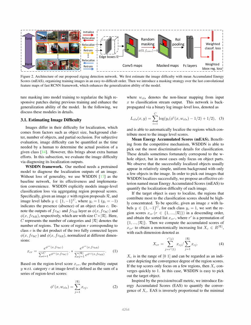
traincarbottle dog chair cat person dingtableFigure 3. Example image difficulty scores by the proposed mEAS metric. Top row: mined object instances and mEAS. Bottom row:
corresponding object heat maps produced by Eq. (7). Best viewed in color.
number of regions needed to make Xc above a threshold t,
EAS(Xc, t) =Xcj[t]
j[t], j[t] = argmin
j
Xcj ≥ t. (5)
It is obvious that a larger EAS(Xc, t) means that fewer re-
gions will be needed to reach the target energy. Finally, we
define the mean Energy Accumulated Scores (mEAS) as the
mean scores at a set of eleven equally spaced energy levels
[0, 0.1, ..., 1]:
mEAS(Xc) =1
11
∑
t∈0,0.1,...,1
EAS(Xc, t). (6)
Mining object instances. Once we obtain the image d-
ifficulty, the remaining task is to mine object instances from
the images. A natural way is to directly choose the top s-
cored region as the target object, which is used for localiza-
tion evaluation in [18]. However, since the whole network
is trained with classification loss, which makes high scored
regions tend to focus on object parts rather than the whole
objects. To relieve this issue, we do not optimistically con-
sider the top scored region to be accurate enough. In con-
trast, we consider them to be accurate enough as soft voters.
To be specific, we compute the object heat map Hc for class
c, which collectively returns the confidence that pixel p lies
in an object, i.e.,
Hc(p) =∑
r
xcrDr(p)/Z, (7)
where Dr(p) = 1 when the r-th region proposal contain-
s pixel p, and Z is a normalization constant such that
maxHc(p)=1. We binarize the heat map Hc with thresh-
old T (set as 0.5 in all experiments), and choose the tightest
bounding box that encloses the largest connect component
as the mined object instance.
Analysis of mEAS. mEAS is an effective criterion to
quantify the localization difficulty of an image. Fig. 3
shows some image difficulty scores from mEAS on PAS-
CAL VOC 2007 dataset, together with the mined object in-
stances (top row) and object heat maps (bottom row). It can
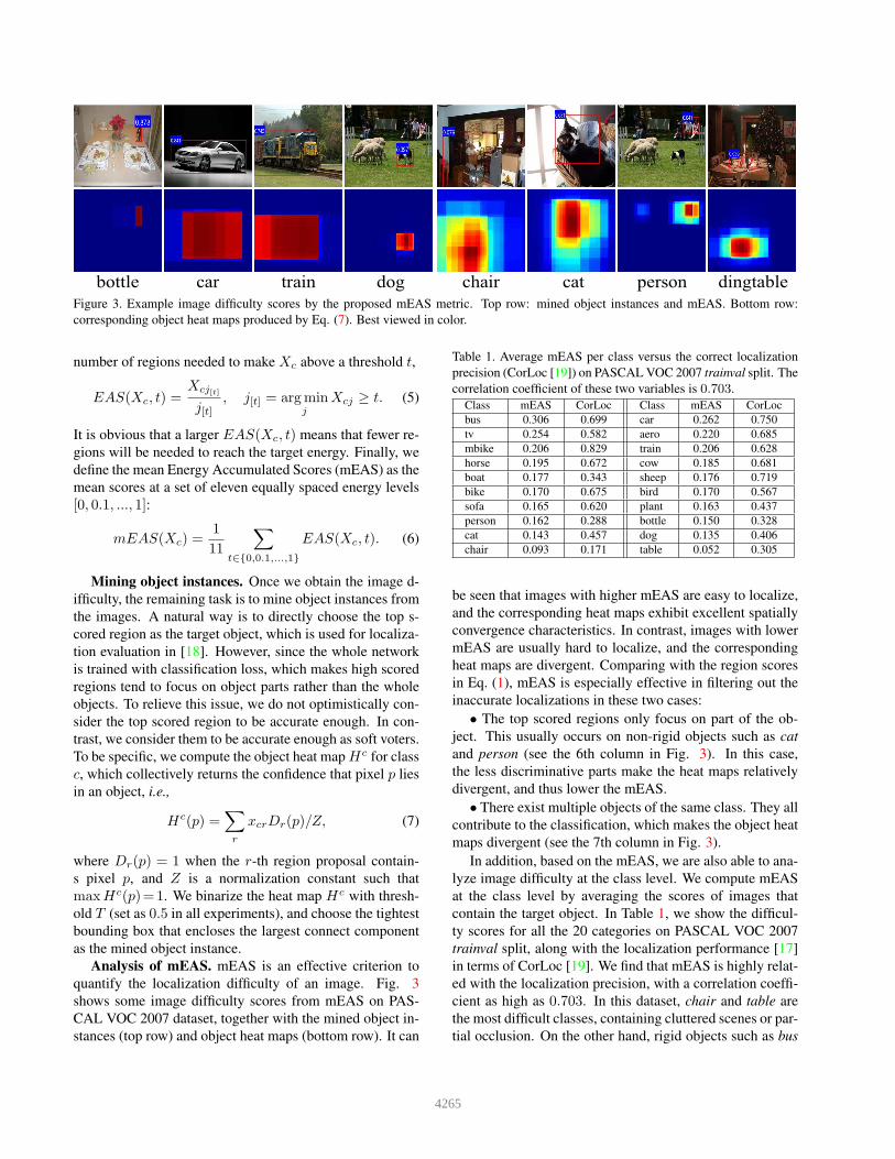
Table 1. Average mEAS per class versus the correct localization
precision (CorLoc [19]) on PASCAL VOC 2007 trainval split. The
correlation coefficient of these two variables is 0.703.
Class mEAS CorLoc Class mEAS CorLoc
bus 0.306 0.699 car 0.262 0.750
tv 0.254 0.582 aero 0.220 0.685
mbike 0.206 0.829 train 0.206 0.628
horse 0.195 0.672 cow 0.185 0.681
boat 0.177 0.343 sheep 0.176 0.719
bike 0.170 0.675 bird 0.170 0.567
sofa 0.165 0.620 plant 0.163 0.437
person 0.162 0.288 bottle 0.150 0.328
cat 0.143 0.457 dog 0.135 0.406
chair 0.093 0.171 table 0.052 0.305
be seen that images with higher mEAS are easy to localize,
and the corresponding heat maps exhibit excellent spatially
convergence characteristics. In contrast, images with lower
mEAS are usually hard to localize, and the corresponding
heat maps are divergent. Comparing with the region scores
in Eq. (1), mEAS is especially effective in filtering out the
inaccurate localizations in these two cases:
• The top scored regions only focus on part of the ob-
ject. This usually occurs on non-rigid objects such as cat
and person (see the 6th column in Fig. 3). In this case,
the less discriminative parts make the heat maps relatively
divergent, and thus lower the mEAS.
• There exist multiple objects of the same class. They all
contribute to the classification, which makes the object heat
maps divergent (see the 7th column in Fig. 3).
In addition, based on the mEAS, we are also able to ana-
lyze image difficulty at the class level. We compute mEAS
at the class level by averaging the scores of images that
contain the target object. In Table 1, we show the difficul-
ty scores for all the 20 categories on PASCAL VOC 2007
trainval split, along with the localization performance [17]
in terms of CorLoc [19]. We find that mEAS is highly relat-
ed with the localization precision, with a correlation coeffi-
cient as high as 0.703. In this dataset, chair and table are
the most difficult classes, containing cluttered scenes or par-
tial occlusion. On the other hand, rigid objects such as bus
4265
Algorithm 1 Zigzag Learning based Weakly Supervised
Detection Network
Input: Training set D = xiNi=1 with image-level labels
Y = yiNi=1, iteration folds K, and masking ratio τ ;
Estimating Image Difficulty: Given an image x with
label y ∈ 1,−1C and region proposals R:
i). Obtain region scores xcr∈RC×|R| with WSDDN.
ii). For each yc = 1, compute mEAS(Xc) with Eq. (6),
and the object instance xoc with Eq. (7).
Progressive Learning: Divide D into K folds D =D1, ...,DK according to mEAS.
for fold k = 1 to K do
i). Training detection model Mk with current selec-
tion of object instances in⋃k
i=1 Di,
a). given an image x, compute the last convolutional
feature maps φ(x, fconv).b). for each mined object instance xo
c , randomly se-
lect regions Ω| SΩ
Sxoc
= τ, and set φ(Ω, fconv) = 0.
c). continue forward and back propagation.
ii). Relocalize object instances in folds⋃k+1
i=1 Di using
current detection model Mk:
end for
Output: Detection models MkKk=1.
and car are the easiest to localize, because these objects are
usually large in images, or in relatively clean background.
3.2. Progressive Detection Network
Given the image difficulty scores and the mined seed
positive instances, we are able to organize our network
training in a progressive learning mode. The detection net-
work follows a fast-RCNN [1] framework. Specifically, we
split the training images D into K folds D = D1, ...,DK,
which are in an easy-to-difficult order. Instead of training
and relocalization on the entire images all at once, we pro-
gressively recruit samples in terms of image difficulty. The
training process starts with running a fast-RCNN on the
first fold D1, which contains the easiest images, and obtains
a trained model MD1. MD1
already has a good general-
ization ability since the trained object instances are highly
reliable. Then we move on to the second fold D2, which
contains relatively more difficult images. Instead of per-
forming training and relocalization from scratch, we choose
the trained model MD1 to discover object instances in fold
D2. It is likely to find more reliable instances on D1
⋃D2.
As the training process proceeds, more images are added
in, which improves the localization ability of the network
steadily. When reaching later folds, the learned model has
been powerful enough for localizing these difficult images.
Weighted loss. Due to the high variation of image dif-
ficulty, the mined object instances used for training cannot
be all reliable. It is suboptimal to treat all these instances
equally important. Therefore, we penalize the output layers
with a weighted loss, which considers the reliability of the
mined instances. At each relocalization step, the network
Mk returns a detection score for each region, indicating it-
s confidence of containing the target object. Formally, let
xoc be the relocalized object with instance label yoc =1, and
φc(xoc ,Mk) be the detection score returned by Mk. The
weighted loss w.r.t. region xoc in the next retraining step is
defined as
Lcls(xoc , y
oc ,Mk+1)=−φc(xo
c ,Mk) log φc(xo
c ,Mk+1). (8)
3.3. Convolutional Feature Masking Regularization
The above detector learning proceeds by alternating be-
tween model retraining and object relocalization, and is
easy to get stuck in sub-optimums without proper initial-
ization. Unfortunately, due to lack of object annotations,
the initial seeds inevitably include inaccurate samples. As
a result, the network tends to overfit those inaccurate in-
stances during each iteration, leading to poor generaliza-
tion. To solve this issue, we propose a regularization strat-
egy to avoid the network from overfitting initial seeds in
the proposed zigzag learning. Concretely, during network
training, we randomly mask out those discriminative details
at previous training, which enforces the network to focus on
those less discriminative details, so that the current network
can see a more holistic object.
The convolutional feature masking operation works as
follows. Given an image x and the mined object xoc for
each yc = 1, we randomly select region Ω ∈ xoc with
SΩ/Sxoc= τ , where SΩ denotes the area of region Ω. As
xoc obtains the highest responses during previous iteration,
Ω is among the most discriminative regions. For each pixel
[u, v] ∈ Ω, we project it onto the last convolutional fea-
ture maps φ(x, fconv), such that the pixel [u, v] in the im-
age domain is closest to the receptive field of that feature
map pixel [u′, v′]. This mapping is complicated due to the
padding operations among convolutional and pooling layer-
s. To simplify the implementation, following [20], we pad
⌊p/2⌋ pixels for each layer with a filter size of p. This estab-
lishes a rough correspondence between a response centered
at [u′, v′], and receptive field in the image domain centered
at [Tu′, T v′], where T is the stride from the image to the
target convolutional feature maps. The mapping of [u, v] to
the feature map [u′, v′] is simply conducted as
u′ = round((u−1)/T+1), v′ = round((v−1)/T+1). (9)
In our experiments, T = 16 for all models. During each
iteration, we randomly mask out the regions by setting
φ(Ω, fconv) = 0, and continue forward and backward prop-
agation as usual. For simplicity, we keep the aspect ratio of
the masked region Ω the same as the mined object xoc . The
whole process is summarized in Algorithm 1.
4266
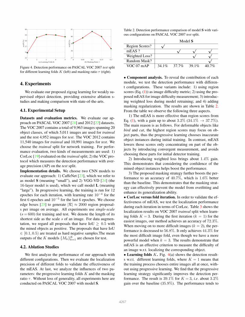
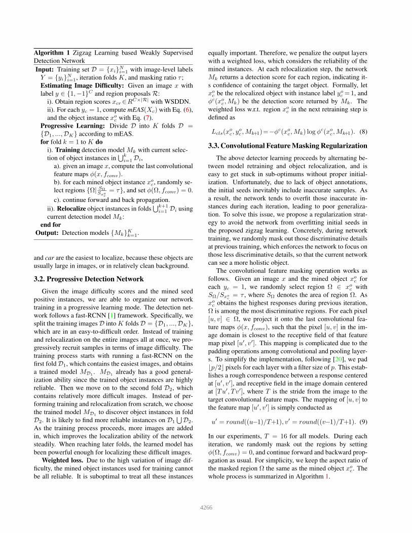
Figure 4. Detection performance on PASCAL VOC 2007 test split
for different learning folds K (left) and masking ratio τ (right).
4. Experiments
We evaluate our proposed zigzag learning for weakly su-
pervised object detection, providing extensive ablation s-
tudies and making comparison with state-of-the-arts.
4.1. Experimental Setup
Datasets and evaluation metrics. We evaluate our ap-
proach on PASCAL VOC 2007 [21] and 2012 [22] datasets.
The VOC 2007 contains a total of 9,963 images spanning 20
object classes, of which 5,011 images are used for trainval
and the rest 4,952 images for test. The VOC 2012 contains
11,540 images for trainval and 10,991 images for test. We
choose the trainval split for network training. For perfor-
mance evaluation, two kinds of measurements are used: 1)
CorLoc [19] evaluated on the trainval split; 2) the VOC pro-
tocol which measures the detection performance with aver-
age precision (AP) on the test split.
Implementation details. We choose two CNN models to
evaluate our approach: 1) CaffeNet [23], which we refer to
as model S (meaning “small”), and 2) VGG-VD [24] (the
16-layer model is used), which we call model L (meaning
“large”). In progressive learning, the training is run for 12epoches for each iteration, with learning rate 10−4 for the
first 6 epoches and 10−5 for the last 6 epoches. We choose
edge boxes [25] to generate |R| ≈ 2000 region proposal-
s per image on average. All experiments use single-scale
(s= 600) for training and test. We denote the length of its
shortest side as the scale s of an image. For data augmen-
tation, we regard all proposals that have IoU ≥ 0.5 with
the mined objects as positive. The proposals that have IoU
∈ [0.1, 0.5) are treated as hard negative samples.The mean
outputs of the K models MkKk=1 are chosen for test.
4.2. Ablation Studies
We first analyze the performance of our approach with
different configurations. Then we evaluate the localization
precision of different folds to validate the effectiveness of
the mEAS. At last, we analyze the influences of two pa-
rameters: the progressive learning folds K and the masking
ratio τ . Without loss of generality, all experiments here are
conducted on PASCAL VOC 2007 with model S.
Table 2. Detection performance comparison of model S with vari-
ous configurations on PASCAL VOC 2007 test split.
Model S
Region Scores?√
mEAS ?√ √ √
Weighted Loss?√ √
Random Mask?√
VOC 07 mAP 34.1% 37.7% 39.1% 40.7%
• Component analysis. To reveal the contribution of each
module, we test the detection performance with differen-
t configurations. These variants include: 1) using region
scores (Eq. (1)) as image difficulty metric; 2) using the pro-
posed mEAS for image difficulty measurement; 3) introduc-
ing weighted loss during model retraining; and 4) adding
masking regularization. The results are shown in Table 2.
From the table we observe the following three aspects.
1) The mEAS is more effective than region scores from
Eq. (1), with a gain up to about 3.2% (34.1% → 37.7%).
The main reason is as follows. For deformable objects like
bird and cat, the highest region scores may focus on ob-
ject parts, thus the progressive learning chooses inaccurate
object instances during initial training. In contrast, mEAS
lowers those scores only concentrating on part of the ob-
jects by introducing convergent measurement, and avoids
choosing these parts for initial detector training.
2) Introducing weighted loss brings about 1.4% gain.
This demonstrates that considering the confidence of the
mined object instances helps boost the performance.
3) The proposed masking strategy further boosts the per-
formance to an accuracy of 40.7%, which is 1.6% better
than the baseline. This demonstrates that the masking strat-
egy can effectively prevent the model from ovetfitting and
enhance its generalization ability.
• CorLoc versus fold iteration. In order to validate the ef-
fectiveness of mEAS, we test the localization performance
during each iteration in terms of CorLoc. Table 3 shows the
localization results on VOC 2007 trainval split when learn-
ing folds K = 3. During the first iteration (k = 1) for the
easiest images, our method achieves an accuracy of 72.3%.
When moving on to more difficult images (k = 2), the per-
formance is decreased to 56.8%. It only achieves 44.3% for
the most difficult image fold, even though we have a more
powerful model when k = 3. The results demonstrate that
mEAS is an effective criterion to measure the difficulty of
an image w.r.t. localizing the corresponding object.
• Learning folds K. Fig. 4(a) shows the detection result-
s w.r.t. different learning folds, where K = 1 means that
the training process chooses entire images all at once, with-
out using progressive learning. We find that the progressive
learning strategy significantly improves the detection per-
formance. The result is 39.1% for K = 3, i.e. about 3.2%gain over the baseline (35.9%). The performance tends to
4267
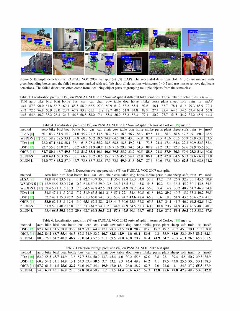
Figure 5. Example detections on PASCAL VOC 2007 test split (47.6% mAP). The successful detections (IoU ≥ 0.5) are marked with
green bounding boxes, and the failed ones are marked with red. We show all detections with scores ≥ 0.7 and use nms to remove duplicate
detections. The failed detections often come from localizing object parts or grouping multiple objects from the same class.
Table 3. Localization precision (%) on PASCAL VOC 2007 trainval split at different fold iterations. The number of total folds is K=3.
Fold aero bike bird boat bottle bus car cat chair cow table dog horse mbike persn plant sheep sofa train tv mAP
k=1 87.3 90.0 81.8 56.7 69.1 85.5 88.9 62.5 27.0 80.9 61.2 53.2 85.4 92.6 36.1 62.7 78.1 81.6 79.3 85.9 72.3
k=2 72.5 76.8 60.9 23.0 20.7 67.7 83.2 61.1 12.8 78.7 48.5 51.8 74.8 88.9 27.4 35.4 64.5 54.6 63.4 67.4 56.8
k=3 64.6 40.7 38.2 28.3 24.7 46.8 68.8 58.0 7.4 55.3 26.9 58.2 58.3 77.1 30.2 27.7 51.5 44.7 32.2 45.9 44.3
Table 4. Localization precision (%) on PASCAL VOC 2007 trainval split in terms of CorLoc [19] metric.
method aero bike bird boat bottle bus car cat chair cow table dog horse mbike persn plant sheep sofa train tv mAP
PLSA [8] 80.1 63.9 51.5 14.9 21.0 55.7 74.2 43.5 26.2 53.4 16.3 56.7 58.3 69.5 14.1 38.3 58.8 47.2 49.1 60.9 48.5
WSDDN [17] 65.1 58.8 58.5 33.1 39.8 68.3 60.2 59.6 34.8 64.5 30.5 43.0 56.8 82.4 25.5 41.6 61.5 55.9 65.9 63.7 53.5
PDA [10] 78.2 67.1 61.8 38.1 36.1 61.8 78.8 55.2 28.5 68.8 18.5 49.2 64.1 73.5 21.4 47.4 64.6 22.3 60.9 52.3 52.4
DSD [12] 72.7 55.3 53.0 27.8 35.2 68.6 81.9 60.7 11.6 71.6 29.7 54.3 64.3 88.2 22.2 53.7 72.2 52.6 68.9 75.5 56.1
OICR [11] 81.7 80.4 48.7 49.5 32.8 81.7 85.4 40.1 40.6 79.5 35.7 33.7 60.5 88.8 21.8 57.9 76.3 59.9 75.3 81.4 60.6
ZLDN-S 74.8 69.1 60.3 35.9 38.1 66.7 80.2 60.5 15.7 71.6 45.5 54.4 72.8 86.1 31.2 42.0 64.6 60.3 58.6 66.4 57.8
ZLDN-L 74.0 77.8 65.2 37.0 46.7 75.8 83.7 58.8 17.5 73.1 49.0 51.3 76.7 87.4 30.6 47.8 75.0 62.5 64.8 68.8 61.2
Table 5. Detection average precision (%) on PASCAL VOC 2007 test split.
method aero bike bird boat bottle bus car cat chair cow table dog horse mbike persn plant sheep sofa train tv mAP
pLSA [8] 48.8 41.0 23.6 12.1 11.1 42.7 40.9 35.5 11.1 36.6 18.4 35.3 34.8 51.3 17.2 17.4 26.8 32.8 35.1 45.6 30.9
WSDDN S [17] 42.9 56.0 32.0 17.6 10.2 61.8 50.2 29.0 3.8 36.2 18.5 31.1 45.8 54.5 10.2 15.4 36.3 45.2 50.1 43.8 34.5
WSDDN L [17] 39.4 50.1 31.5 16.3 12.6 64.5 42.8 42.6 10.1 35.7 24.9 38.2 34.4 55.6 9.4 14.7 30.2 40.7 54.7 46.9 34.8
PDA [10] 54.5 47.4 41.3 20.8 17.7 51.9 63.5 46.1 21.8 57.1 22.1 34.4 50.5 61.8 16.2 29.9 40.7 15.9 55.3 40.2 39.5
DSD [12] 52.2 47.1 35.0 26.7 15.4 61.3 66.0 54.3 3.0 53.6 24.7 43.6 48.4 65.8 6.6 18.8 51.9 43.6 53.6 62.4 41.7
OICR [11] 58.0 62.4 31.1 19.4 13.0 65.1 62.2 28.4 24.8 44.7 30.6 25.3 37.8 65.5 15.7 24.1 41.7 46.9 64.3 62.6 41.2
ZLDN-S 51.9 57.5 40.9 15.8 17.6 53.3 61.2 54.0 2.0 44.2 42.9 34.5 58.3 60.3 18.8 20.7 44.9 43.4 43.5 48.3 40.7
ZLDN-L 55.4 68.5 50.1 16.8 20.8 62.7 66.8 56.5 2.1 57.8 47.5 40.1 69.7 68.2 21.6 27.2 53.4 56.1 52.5 58.2 47.6
Table 6. Localization precision (%) on PASCAL VOC 2012 trainval split in terms of CorLoc [19] metric.
method aero bike bird boat bottle bus car cat chair cow table dog horse mbike persn plant sheep sofa train tv mAP
DSD [12] 82.4 68.1 54.5 38.9 35.9 84.7 73.1 64.8 17.1 78.3 22.5 57.0 70.8 86.6 18.7 49.7 80.7 45.3 70.1 77.3 58.8
OICR [11] 86.2 84.2 68.7 55.4 46.5 82.8 74.9 32.2 46.7 82.8 42.9 41.0 68.1 89.6 9.2 53.9 81.0 52.9 59.5 83.2 62.1
ZLDN-L 80.3 76.5 64.2 40.9 46.7 78.0 84.3 57.6 21.1 69.5 28.0 46.8 70.7 89.4 41.9 54.7 76.3 61.1 76.3 65.2 61.5
Table 7. Detection average precision (%) on PASCAL VOC 2012 test split.
method aero bike bird boat bottle bus car cat chair cow table dog horse mbike persn plant sheep sofa train tv mAP
PDA [10] 62.9 55.5 43.7 14.9 13.6 57.7 52.4 50.9 13.3 45.4 4.0 30.2 55.6 67.0 3.8 23.1 39.4 5.5 50.7 29.3 35.9
DSD [12] 60.8 54.2 34.1 14.9 13.1 54.3 53.4 58.6 3.7 53.1 8.3 43.4 49.8 69.2 4.1 17.5 43.8 25.6 55.0 50.1 38.3
OICR [11] 67.7 61.2 41.5 25.6 22.2 54.6 49.7 25.4 19.9 47.0 18.1 26.0 38.9 67.7 2.0 22.6 41.1 34.3 37.9 55.3 37.9
ZLDN-L 54.3 63.7 43.1 16.9 21.5 57.8 60.4 50.9 1.2 51.5 44.4 36.6 63.6 59.3 12.8 25.6 47.8 47.2 48.9 50.6 42.9
4268
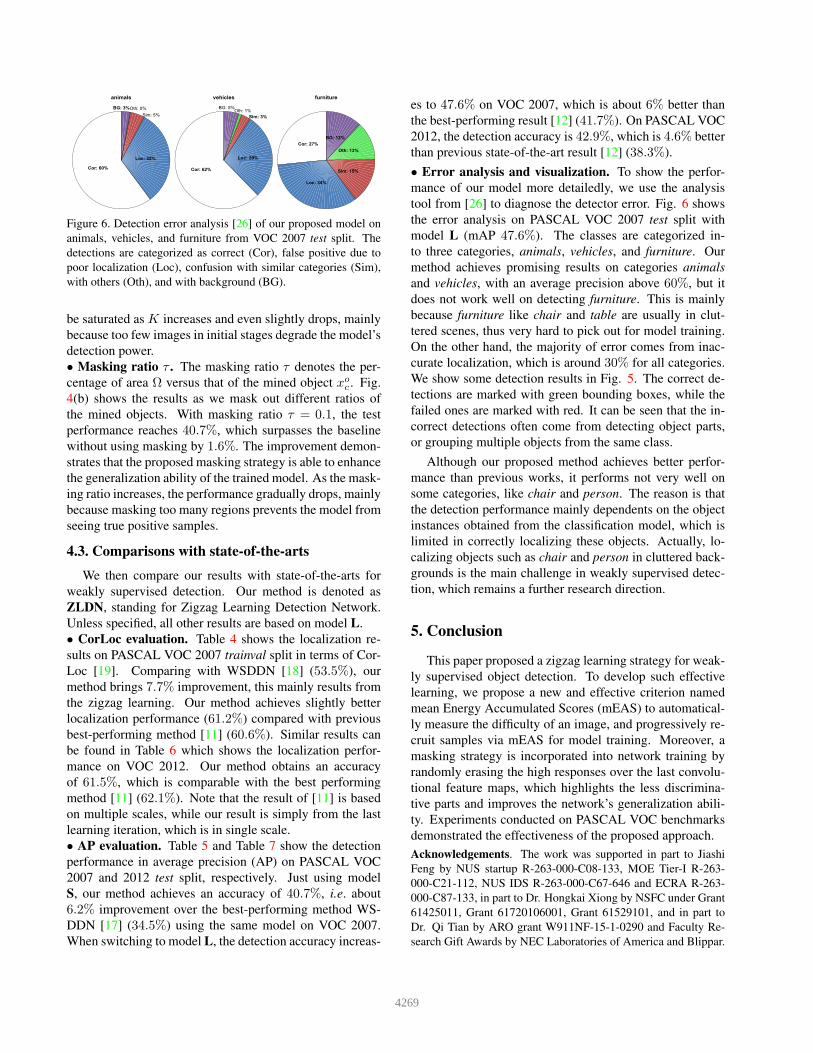
Figure 6. Detection error analysis [26] of our proposed model on
animals, vehicles, and furniture from VOC 2007 test split. The
detections are categorized as correct (Cor), false positive due to
poor localization (Loc), confusion with similar categories (Sim),
with others (Oth), and with background (BG).
be saturated as K increases and even slightly drops, mainly
because too few images in initial stages degrade the model’s
detection power.
• Masking ratio τ . The masking ratio τ denotes the per-
centage of area Ω versus that of the mined object xoc . Fig.
4(b) shows the results as we mask out different ratios of
the mined objects. With masking ratio τ = 0.1, the test
performance reaches 40.7%, which surpasses the baseline
without using masking by 1.6%. The improvement demon-
strates that the proposed masking strategy is able to enhance
the generalization ability of the trained model. As the mask-
ing ratio increases, the performance gradually drops, mainly
because masking too many regions prevents the model from
seeing true positive samples.
4.3. Comparisons with stateofthearts
We then compare our results with state-of-the-arts for
weakly supervised detection. Our method is denoted as
ZLDN, standing for Zigzag Learning Detection Network.
Unless specified, all other results are based on model L.
• CorLoc evaluation. Table 4 shows the localization re-
sults on PASCAL VOC 2007 trainval split in terms of Cor-
Loc [19]. Comparing with WSDDN [18] (53.5%), our
method brings 7.7% improvement, this mainly results from
the zigzag learning. Our method achieves slightly better
localization performance (61.2%) compared with previous
best-performing method [11] (60.6%). Similar results can
be found in Table 6 which shows the localization perfor-
mance on VOC 2012. Our method obtains an accuracy
of 61.5%, which is comparable with the best performing
method [11] (62.1%). Note that the result of [11] is based
on multiple scales, while our result is simply from the last
learning iteration, which is in single scale.
• AP evaluation. Table 5 and Table 7 show the detection
performance in average precision (AP) on PASCAL VOC
2007 and 2012 test split, respectively. Just using model
S, our method achieves an accuracy of 40.7%, i.e. about
6.2% improvement over the best-performing method WS-
DDN [17] (34.5%) using the same model on VOC 2007.
When switching to model L, the detection accuracy increas-
es to 47.6% on VOC 2007, which is about 6% better than
the best-performing result [12] (41.7%). On PASCAL VOC
2012, the detection accuracy is 42.9%, which is 4.6% better
than previous state-of-the-art result [12] (38.3%).
• Error analysis and visualization. To show the perfor-
mance of our model more detailedly, we use the analysis
tool from [26] to diagnose the detector error. Fig. 6 shows
the error analysis on PASCAL VOC 2007 test split with
model L (mAP 47.6%). The classes are categorized in-
to three categories, animals, vehicles, and furniture. Our
method achieves promising results on categories animals
and vehicles, with an average precision above 60%, but it
does not work well on detecting furniture. This is mainly
because furniture like chair and table are usually in clut-
tered scenes, thus very hard to pick out for model training.
On the other hand, the majority of error comes from inac-
curate localization, which is around 30% for all categories.
We show some detection results in Fig. 5. The correct de-
tections are marked with green bounding boxes, while the
failed ones are marked with red. It can be seen that the in-
correct detections often come from detecting object parts,
or grouping multiple objects from the same class.
Although our proposed method achieves better perfor-
mance than previous works, it performs not very well on
some categories, like chair and person. The reason is that
the detection performance mainly dependents on the object
instances obtained from the classification model, which is
limited in correctly localizing these objects. Actually, lo-
calizing objects such as chair and person in cluttered back-
grounds is the main challenge in weakly supervised detec-
tion, which remains a further research direction.
5. Conclusion
This paper proposed a zigzag learning strategy for weak-
ly supervised object detection. To develop such effective
learning, we propose a new and effective criterion named
mean Energy Accumulated Scores (mEAS) to automatical-
ly measure the difficulty of an image, and progressively re-
cruit samples via mEAS for model training. Moreover, a
masking strategy is incorporated into network training by
randomly erasing the high responses over the last convolu-
tional feature maps, which highlights the less discrimina-
tive parts and improves the network’s generalization abili-
ty. Experiments conducted on PASCAL VOC benchmarks
demonstrated the effectiveness of the proposed approach.
Acknowledgements. The work was supported in part to Jiashi
Feng by NUS startup R-263-000-C08-133, MOE Tier-I R-263-
000-C21-112, NUS IDS R-263-000-C67-646 and ECRA R-263-
000-C87-133, in part to Dr. Hongkai Xiong by NSFC under Grant
61425011, Grant 61720106001, Grant 61529101, and in part to
Dr. Qi Tian by ARO grant W911NF-15-1-0290 and Faculty Re-
search Gift Awards by NEC Laboratories of America and Blippar.
4269
References
[1] R. Girshick, “Fast r-cnn,” in ICCV, pp. 1440–1448, 2015. 1,
5
[2] W. Liu, D. Anguelov, D. Erhan, C. Szegedy, S. Reed, C.-Y.
Fu, and A. C. Berg, “Ssd: Single shot multibox detector,” in
ECCV, pp. 21–37, 2016. 1
[3] J. Redmon, S. Divvala, R. Girshick, and A. Farhadi, “You on-
ly look once: Unified, real-time object detection,” in CVPR,
pp. 779–788, 2016. 1
[4] L. Niu, W. Li, and D. Xu, “Visual recognition by learning
from web data: A weakly supervised domain generalization
approach,” in CVPR, pp. 2774–2783, 2015. 1
[5] S. Vijayanarasimhan and K. Grauman, “Keywords to visual
categories: Multiple-instance learning forweakly supervised
object categorization,” in CVPR, pp. 1–8, 2008. 1
[6] Y. Li, L. Liu, C. Shen, and A. v. d. Hengel, “Image co-
localization by mimicking a good detector’s confidence score
distribution,” arXiv preprint arXiv:1603.04619, 2016. 1
[7] H. O. Song, Y. J. Lee, S. Jegelka, and T. Darrell, “Weakly-
supervised discovery of visual pattern configurations,” in
NIPS, pp. 1637–1645, 2014. 1, 2
[8] C. Wang, W. Ren, K. Huang, and T. Tan, “Weakly supervised
object localization with latent category learning,” in ECCV,
pp. 431–445, 2014. 1, 2, 7
[9] R. G. Cinbis, J. Verbeek, and C. Schmid, “Multi-fold mil
training for weakly supervised object localization,” in CVPR,
pp. 2409–2416, 2014. 1, 2
[10] D. Li, J.-B. Huang, Y. Li, S. Wang, and M.-H. Yang, “Weakly
supervised object localization with progressive domain adap-
tation,” in CVPR, pp. 3512–3520, 2016. 1, 2, 7
[11] P. Tang, X. Wang, X. Bai, and W. Liu, “Multiple instance
detection network with online instance classifier refinement,”
in CVPR, pp. 2843–2850, 2017. 1, 2, 7, 8
[12] Z. Jie, Y. Wei, X. Jin, J. Feng, and W. Liu, “Deep self-taught
learning for weakly supervised object localization,” CVPR,
pp. 1377–1385, 2017. 1, 7, 8
[13] M. P. Kumar, B. Packer, and D. Koller, “Self-paced learning
for latent variable models,” in NIPS, pp. 1189–1197, 2010. 1
[14] R. Tudor Ionescu, B. Alexe, M. Leordeanu, M. Popescu,
D. P. Papadopoulos, and V. Ferrari, “How hard can it be?
estimating the difficulty of visual search in an image,” in
CVPR, pp. 2157–2166, 2016. 2, 3
[15] M. Shi and V. Ferrari, “Weakly supervised object localization
using size estimates,” in ECCV, pp. 105–121, 2016. 2
[16] M. Oquab, L. Bottou, I. Laptev, and J. Sivic, “Is object lo-
calization for free?-weakly-supervised learning with convo-
lutional neural networks,” in CVPR, pp. 685–694, 2015. 2
[17] H. Bilen and A. Vedaldi, “Weakly supervised deep detection
networks,” in CVPR, pp. 2846–2854, 2016. 2, 3, 4, 7, 8
[18] A. J. Bency, H. Kwon, H. Lee, S. Karthikeyan, and B. Man-
junath, “Weakly supervised localization using deep feature
maps,” arXiv preprint arXiv:1603.00489, 2016. 2, 4, 8
[19] T. Deselaers, B. Alexe, and V. Ferrari, “Weakly supervised
localization and learning with generic knowledge,” IJCV,
vol. 100, no. 3, pp. 275–293, 2012. 4, 6, 7, 8
[20] K. He, X. Zhang, S. Ren, and J. Sun, “Spatial pyramid pool-
ing in deep convolutional networks for visual recognition,”
in ECCV, pp. 346–361, 2014. 5
[21] M. Everingham, L. Van Gool, C. K. Williams, J. Winn, and
A. Zisserman, “The pascal visual object classes (voc) chal-
lenge,” IJCV, vol. 88, no. 2, pp. 303–338, 2010. 6
[22] M. Everingham, S. A. Eslami, L. Van Gool, C. K. Williams,
J. Winn, and A. Zisserman, “The pascal visual object classes
challenge: A retrospective,” IJCV, vol. 111, no. 1, pp. 98–
136, 2015. 6
[23] Y. Jia, E. Shelhamer, J. Donahue, S. Karayev, J. Long, R. Gir-
shick, S. Guadarrama, and T. Darrell, “Caffe: Convolutional
architecture for fast feature embedding,” in ACM Multimedi-
a, pp. 675–678, 2014. 6
[24] K. Simonyan and A. Zisserman, “Very deep convolutional
networks for large-scale image recognition,” CoRR, vol. ab-
s/1409.1556, 2014. 6
[25] C. L. Zitnick and P. Dollar, “Edge boxes: Locating object
proposals from edges,” in ECCV, pp. 391–405, 2014. 6
[26] D. Hoiem, Y. Chodpathumwan, and Q. Dai, “Diagnosing er-
ror in object detectors,” in ECCV, pp. 340–353, 2012. 8
4270