Discrete Mathematics 309 (2009) 5596–5609

Contents lists available at ScienceDirect

Discrete Mathematics

journal homepage: www.elsevier.com/locate/disc

λ-backbone colorings along pairwise disjoint stars and matchingsH.J. Broersma a,∗, J. Fujisawa b, L. Marchal c, D. Paulusma a, A.N.M. Salman d, K. Yoshimoto e

a Department of Computer Science, Durham University, South Road, DH1 3LE, Durham, United Kingdomb Department of Computer Science, Nihon University, Sakurajosui 3-25-40, Setagaya-Ku, Tokyo 156-8550, Japanc Quantitative Economics, Maastricht University, P.O. Box 616, 6200 MD Maastricht, The Netherlandsd Combinatorial Mathematics Research Group, Faculty of Mathematics and Natural Sciences, Institut Teknologi Bandung,Jalan Ganesa 10 Bandung 40132, Indonesiae Department of Mathematics, College of Science and Technology, Nihon University, 1-8 Kanda-Surugadai, Chiyoda-ku, Tokyo, 101-8308, Japan

a r t i c l e i n f o

Article history:Received 4 August 2006Accepted 1 April 2008Available online 14 May 2008

Keywords:λ-backbone coloringλ-backbone coloring numberStarMatching

a b s t r a c t

Given an integer λ ≥ 2, a graph G = (V, E) and a spanning subgraph H of G (the backbone ofG), a λ-backbone coloring of (G,H) is a proper vertex coloring V → {1, 2, . . .} of G, in whichthe colors assigned to adjacent vertices in H differ by at least λ. We study the case wherethe backbone is either a collection of pairwise disjoint stars or a matching. We show thatfor a star backbone S of G the minimum number ` for which a λ-backbone coloring of (G, S)with colors in {1, . . . , `} exists can roughly differ by a multiplicative factor of at most 2− 1

λfrom the chromatic number χ(G). For the special case of matching backbones this factor isroughly 2− 2

λ+1 . We also show that the computational complexity of the problem “Given agraphGwith a star backbone S, and an integer `, is there aλ-backbone coloring of (G, S) withcolors in {1, . . . , `}?” jumps from polynomially solvable toNP-complete between ` = λ+1and ` = λ+2 (the case ` = λ+2 is even NP-complete for matchings). We finish the paperby discussing some open problems regarding planar graphs.

© 2008 Elsevier B.V. All rights reserved.

1. Introduction

In [7] backbone colorings are introduced, motivated and put into a general framework of coloring problems related tofrequency assignment.

Graphs are used to model the topology and interference between transmitters (receivers, base stations, sensors): thevertices represent the transmitters; two vertices are adjacent if the corresponding transmitters are so close (or so strong)that they are likely to interfere if they broadcast on the same or ‘similar’ frequency channels. The problem is to assign thefrequency channels in an economical way to the transmitters in such a way that interference is kept at an ‘acceptable level’.This has led to various types of coloring problems in graphs, depending on different ways to model the level of interference,the notion of similar frequency channels, and the definition of acceptable level of interference (see, e.g., [16,20]). Althoughnew technologies have led to different ways of avoiding interference between powerful transmitters, such as base stationsfor mobile telephones, the above coloring problems still apply to less powerful transmitters, such as those appearing insensor networks.

We refer the reader to [6,7] for an overview of related research, but we repeat the general framework and some of therelated research here for convenience and background.

∗ Corresponding author.E-mail addresses: hajo.broersma@durham.ac.uk (H.J. Broersma), fujisawa@cs.chs.nihon-u.ac.jp (J. Fujisawa), b.marchal@ke.unimaas.nl (L. Marchal),

daniel.paulusma@durham.ac.uk (D. Paulusma), msalman@math.itb.ac.id (A.N.M. Salman), yosimoto@math.cst.nihon-u.ac.jp (K. Yoshimoto).

0012-365X/$ – see front matter © 2008 Elsevier B.V. All rights reserved.doi:10.1016/j.disc.2008.04.007

H.J. Broersma et al. / Discrete Mathematics 309 (2009) 5596–5609 5597

Given two graphs G1 and G2 with the property that G1 is a spanning subgraph of G2, one considers the following type ofcoloring problems: Determine a coloring of (G1 and) G2 that satisfies certain restrictions of type 1 in G1, and restrictionsof type 2 in G2.

Many known coloring problems fit into this general framework. We mention some of them here explicitly, without givingdetails. First of all suppose that G2 = G2

1, i.e. G2 is obtained from G1 by adding edges between all pairs of vertices that are atdistance 2 in G1. If one just asks for a proper vertex coloring of G2 (and G1), this is known as the distance-2-coloring problem.Much of the research has been concentrated on the case that G1 is a planar graph. We refer to [1,4,5,18,21] for more details.In some versions of this problem one puts the additional restriction on G1 that the colors should be sufficiently separated, inorder to model practical frequency assignment problems in which interference should be kept at an acceptable level. Oneway to model this is to use positive integers for the colors (modeling certain frequency channels) and to ask for a coloringof G1 and G2 such that the colors on adjacent vertices in G2 are different, whereas they differ by at least 2 on adjacentvertices in G1. A closely related variant is known as the radio coloring problem and has been studied (under various names)in [2,9–13,19]. A third variant is known as the radio labeling problem and models a practical setting in which all assignedfrequency channels should be distinct, with the additional restriction that adjacent transmitters should use sufficientlyseparated frequency channels. Within the above framework this can be modeled by considering the graph G1 that modelsthe adjacencies of n transmitters, and taking G2 = Kn, the complete graph on n vertices. The restrictions are clear: one asksfor a proper vertex coloring of G2 such that adjacent vertices in G1 receive colors that differ by at least 2. We refer to [15,17]for more particulars.

In [7], a situation is modeled in which the transmitters form a network in which a certain substructure of adjacenttransmitters (called the backbone) is more crucial for the communication than the rest of the network. This means morerestrictions are put on the assignment of frequency channels along the backbone than on the assignment of frequencychannels to other adjacent transmitters.

Postponing the relevant definitions, we consider the problem of coloring the graph G2 (that models the whole network)with a proper vertex coloring such that the colors on adjacent vertices in G1 (that models the backbone) differ by at leastλ ≥ 2. This is a continuation of the study in [7]. Throughout the paper we consider two types of backbones: matchings anddisjoint unions of stars.

Matching backbones reflect the necessity to assign considerably different frequencies to pairwise very close (or mostlikely interfering) transmitters. This occurs in real world applications such as military scenarios, where soldiers or militaryvehicles carry two (or sometimes more) radios for reliable communication. Future applications include the use of sensorsor sensor tags in clothes or on bodies.

For star backbones one could think of applications to sensor networks. If sensors have low battery capacities, the tasksof transmitting data are often assigned to specific sensors, called cluster heads, that represent pairwise disjoint clusters ofsensors. Within the clusters there should be a considerable difference between the frequencies assigned to the cluster headand to the other sensors within the same cluster, whereas the differences between the frequencies assigned to the othersensors within the cluster, or between different clusters, are of secondary importance. This situation is well reflected by abackbone consisting of disjoint stars.

We refer the reader to [7,6] for a more extensive overview of related research, but we repeat the relevant definitions inthe next section.

2. Terminology

For undefined terminology we refer to [3].Let G = (V, E) be a graph, where V = VG is a finite set of vertices and E = EG is a set of unordered pairs of two different

vertices, called edges. A function f : V → {1, 2, 3, . . .} is a vertex coloring of V if |f (u)− f (v)| ≥ 1 holds for all edges uv ∈ E. Avertex coloring f : V → {1, . . . , k} is called a k-coloring. We say that f (u) is the color of u. The chromatic number χ(G) is thesmallest integer k for which there exists a k-coloring. A set V ′ ⊆ V is independent if G does not contain edges with both endvertices in V ′. By definition, a k-coloring partitions V into k independent sets V1, . . . , Vk.

Let H be a spanning subgraph of G, i.e., H = (VG, EH) with EH ⊆ EG. Given an integer λ ≥ 1, a vertex coloring f is a λ-backbone coloring of (G,H), if |f (u)− f (v)| ≥ λ holds for all edges uv ∈ EH . A λ-backbone coloring f : V → {1, . . . , `} is calleda λ-backbone `-coloring. The λ-backbone coloring number bbcλ(G,H) of (G,H) is the smallest integer ` for which there existsa λ-backbone `-coloring. Since a 1-backbone coloring is equivalent to a vertex coloring, we assume from now on that λ ≥ 2.Throughout the manuscript we will reserve the symbol “`” for λ-backbone `-colorings and the symbol “k” for k-colorings.

A path is a graph P whose vertices can be ordered into a sequence v1, v2, . . . , vn such that EP = {v1v2, . . . , vn−1vn}. A graphG is called connected if for every pair of distinct vertices u and v, there exists a path connecting u and v. The length of a pathis the number of its edges. If a graph G contains a spanning subgraph H that is a path, then H is called a Hamiltonian path.

A cycle is a graph C whose vertices can be ordered into a sequence v1, v2, . . . , vn such that EC = {v1v2, . . . , vn−1vn, vnv1}. Atree is a connected graph that does not contain any cycles.

A complete graph is a graph with an edge between every pair of vertices. The complete graph on n vertices is denotedby Kn. A graph is called bipartite if its vertices can be partitioned into two sets A and B such that each edge has one of its

5598 H.J. Broersma et al. / Discrete Mathematics 309 (2009) 5596–5609

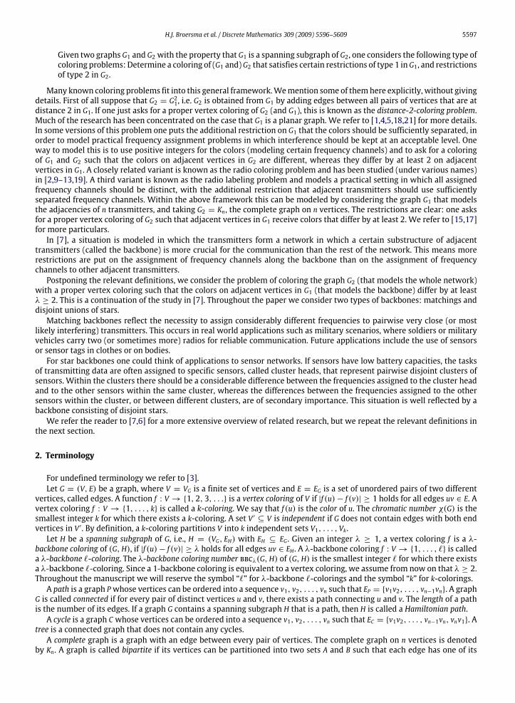
Fig. 1. Matching and star backbones.

endpoints incident with the set A and the other with B. A graph G is complete p-partite if its vertices can be partitioned into pnonempty independent sets V1, . . . , Vp such that its edge set E is formed by all edges that have one end vertex in Vi and theother one in Vj for some 1 ≤ i < j ≤ p.

For q ≥ 1, a star Sq is a complete 2-partite graph with independent sets V1 = {r} and V2 with |V2| = q; the vertex r is calledthe root and the vertices in V2 are called the leaves of Sq. For the star S1 we arbitrarily choose one of its two vertices to be theroot. In our context a matching M is a collection of pairwise vertex-disjoint stars that are all copies of S1. A matching M of agraph G is called perfect if it is a spanning subgraph of G.

We call a spanning subgraph H of a graph G

• a tree backbone of G if H is a tree;• a path backbone of G if H is a Hamiltonian path;• a star backbone of G if H is a collection of pairwise vertex-disjoint stars;• a matching backbone of G if H is a perfect matching.

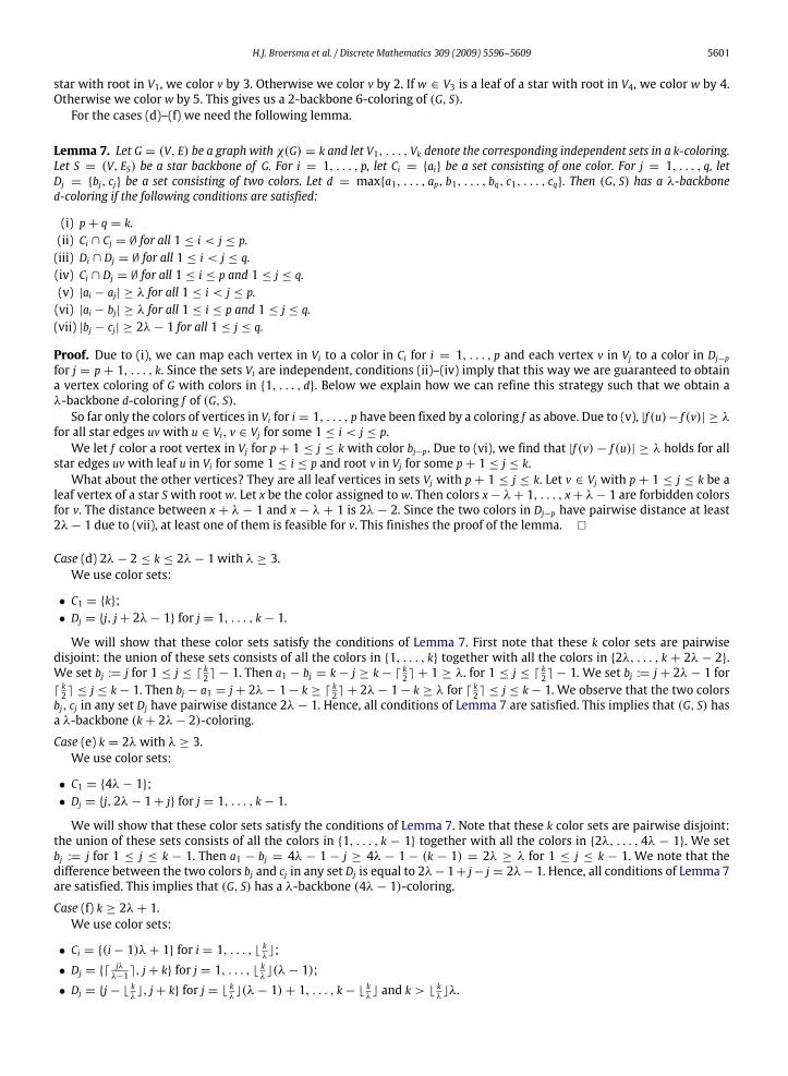
See Fig. 1 for an example of a graph G with a matching backbone M (left) and a star backbone S (right). The thick edgesare matching or star edges, respectively. The grey circles indicate root vertices of the stars in S.

Obviously, bbcλ(G,H) ≥ χ(G) holds for any backbone H of a graph G. In order to analyze the maximum difference betweenthese two numbers the following values can be introduced.

Tλ(k) = max{bbcλ(G, T) | T is a tree backbone of G, and χ(G) = k

}Pλ(k) = max

{bbcλ(G, P) | P is a path backbone of G, and χ(G) = k

}Sλ(k) = max

{bbcλ(G, S) | S is a star backbone of G, and χ(G) = k

}Mλ(k) = max

{bbcλ(G,M) | M is a matching backbone of G, and χ(G) = k

}.

3. Results

3.1. Existing results

The behavior of Tλ(k) and Pλ(k) is determined in [7] as summarized in the following two results.

Theorem 1. T2(k) = 2k− 1 for all k ≥ 1.

Theorem 2. The function P2(k) takes the following values:

(a) for 1 ≤ k ≤ 4 : P2(k) = 2k− 1;(b) P2(5) = 8 and P2(6) = 10;(c) for k ≥ 7 and k = 4t : P2(4t) = 6t;(d) for k ≥ 7 and k = 4t + 1 : P2(4t + 1) = 6t + 1;(e) for k ≥ 7 and k = 4t + 2 : P2(4t + 2) = 6t + 3;(f) for k ≥ 7 and k = 4t + 3 : P2(4t + 3) = 6t + 5.

The above theorems show the relation between the 2-backbone coloring number and the classical chromatic number incase the backbone is a tree or a path. We observe that in the worst case the 2-backbone coloring number roughly grows like2k and 3k/2, respectively, where χ = k.

Problem 3. What are the values for Tλ(k) and Pλ(k) for λ ≥ 3?

H.J. Broersma et al. / Discrete Mathematics 309 (2009) 5596–5609 5599

3.2. Results of this paper

In this paper, we study the functions Sλ(k) and Mλ(k). By definition, Mλ(k) ≤ Sλ(k) holds. We completely determine thebehavior of these two functions. We first determine all values Sλ(k), and observe that they roughly grow like (2− 1

λ)k. Then

we determine all values Mλ(k) and observe that they roughly grow like (2 − 2λ+1 )k. Their precise behavior is summarized

in our two main theorems.

Theorem 4. For λ ≥ 2 the function Sλ(k) takes the following values:

(a) Sλ(2) = λ+ 1;(b) for 3 ≤ k ≤ 2λ− 3 : Sλ(k) = d

3k2 e + λ− 2;

(c) for 2λ− 1 ≤ k ≤ 2λ with λ = 2 : Sλ(k) = k+ 2λ− 2;(d) for 2λ− 2 ≤ k ≤ 2λ− 1 with λ ≥ 3 : Sλ(k) = k+ 2λ− 2;(e) for k = 2λ with λ ≥ 3 : Sλ(k) = 2k− 1;(f) for k ≥ 2λ+ 1 : Sλ(k) = 2k− b k

λc.

Theorem 5. For λ ≥ 2 the function Mλ(k) takes the following values:

(a) for 2 ≤ k ≤ λ : Mλ(k) = k+ λ− 1;(b) for λ+ 1 ≤ k ≤ 2λ : Mλ(k) = 2k− 2;(c) for k = 2λ+ 1 : Mλ(k) = 2k− 3;(d) for k = t(λ+ 1) with t ≥ 2 : Mλ(k) = 2tλ;(e) for k = t(λ+ 1)+ c with t ≥ 2, 1 ≤ c < λ+3

2 : Mλ(k) = 2tλ+ 2c− 1;(f) for k = t(λ+ 1)+ c with t ≥ 2, λ+3

2 ≤ c ≤ λ : Mλ(k) = 2tλ+ 2c− 2.

We note that there are many graphs G that have a star backbone S such that bbcλ(G, S) < Sλ(χ(G)), or that have a matchingbackbone M such that bbcλ(G,M) < Mλ(χ(G)). As an example we mention the class of split graphs, e.g., graphs whose vertexset can be partitioned into a clique (i.e., a set of pairwise adjacent vertices) and an independent set, with possibly edges inbetween. In [8] we present (tight) upper bounds on the λ-star and λ-matching backbone coloring number for this graphclass. These upper bounds are considerably smaller than the general bounds given in Theorems 4 and 5, respectively.

The rest of the paper is organized as follows. In the next section we consider the computational complexity of computingthe λ-backbone coloring number for star and matching backbones. The fifth section gives the proof of Theorem 4, and thesixth section gives the proof of Theorem 5. There are many open problems about backbone colorings. We refer to [7] fordetails. In the last section of this paper we only focus on some open problems for matching backbone colorings for planargraphs.

4. Complexity results

The following decision problem can be defined.λ-Backbone Colorability (`) (λ-BBC (`))Instance: A graph G with a spanning subgraph H.Question: Is bbcλ(G,H) ≤ `?

Of course, λ-BBC (`) is NP-complete if ` exceeds a certain value. In [7] it has been shown that the complexity of 2-BBC(`) restricted to instance graphs G with a tree backbone H jumps from polynomially solvable toNP-complete between ` = 4and ` = 5 (difficult even for path backbones). Here we restrict ourselves to instance graphs G with a star backbone S.Star λ-Backbone Colorability (`) (λ-SBBC (`))Instance: A graph G with a star backbone S.Question: Is bbcλ(G, S) ≤ `?

Theorem 6. λ-SBBC (`) is polynomially solvable if ` ≤ λ + 1, and it is NP-complete if ` ≥ λ + 2 (even when restricted tomatching backbones).

Proof. Let G = (V, E) be a graph with a star backbone S = (V, ES). For ` ≤ λ no λ-backbone coloring exists. Now let` = λ + 1. In any λ-backbone coloring with color set {1, 2, . . . ,λ + 1}, colors 2, 3, . . . ,λ cannot be used at all, since eachvertex is incident with an edge of ES. Hence bbcλ(G, S) = λ+ 1 if and only if G is bipartite.

Let ` ≥ λ + 2. Obviously the problem λ-SBBC (`) is a member of NP. We prove NP-completeness by reduction fromGraph k-Colorability (cf. [14]): Given a graph G = (VG, EG), does there exist a k-coloring of G? This problem is known to beNP-complete for any integer k ≥ 3. We distinguish the following cases.Case 1 λ+ 2 ≤ ` ≤ 2λ− 1.

Let ` = λ + t for some 2 ≤ t ≤ λ − 1, and let G = (VG, EG) be an instance of Graph 2t-Colorability. Let v1, v2, . . . , vndenote the vertices in VG. We create n new vertices u1, u2, . . . , un and introduce new edges viui (i = 1, 2, . . . , n). The graph

5600 H.J. Broersma et al. / Discrete Mathematics 309 (2009) 5596–5609

that results from this is denoted by G′. The new edges form a matching backbone M of G′. We claim that χ(G) ≤ 2t if andonly if bbcλ(G′,M) ≤ `.

Assume that bbcλ(G′,M) ≤ `, and consider a λ-backbone `-coloring b of G′. Since all vertices in G′ are incident with amatching edge, colors t + 1, t + 2, . . . ,λ cannot be used at all. Then define a 2t-coloring c of G by:

• if b(v) = j for j ∈ {1, 2, . . . , t}: c(v) := j;• if b(v) = λ+ j for j ∈ {1, 2, . . . , t}: c(v) := t + j.

Next, assume that χ(G) ≤ 2t, and consider a 2t-coloring f : VG → {1, . . . , 2t}. We define a λ-backbone `-coloringg : VG′ → {1, . . . , `} of (G′,M) by:

• if v ∈ VG and f (v) = j for j ∈ {1, 2, . . . , t}: g(v) := j;• if v ∈ VG and f (v) = t + j for j ∈ {1, 2, . . . , t}: g(v) := λ+ j;• if g(vi) ≤ t: g(ui) := `;• If g(vi) ≥ λ+ 1: g(ui) := 1.

Case 2 ` ≥ 2λ.Let G = (VG, EG) be an instance of Graph `-Colorability, and denote the vertices in VG by v1, v2, . . . , vn. We create n new

vertices u1, u2, . . . , un and introduce new edges viui (i = 1, 2, . . . , n). The graph that results from this is denoted by G′. Thenew edges form a matching backbone M of G′. We complete the proof by showing thatχ(G) ≤ ` if and only if bbcλ(G′,M) ≤ `.

Indeed, assume that bbcλ(G′,M) ≤ ` and consider such a λ-backbone `-coloring. Then the restriction to the vertices inVG yields an `-coloring of G. Next assume that χ(G) ≤ `, and consider an `-coloring f : VG → {1, . . . , `}. We extend f to aλ-backbone `-coloring of (G′,M): If f (vi) ≤ λ, then vertex ui is colored with color `, and otherwise it is assigned color 1. Thiscompletes the proof. �

5. Proof of Theorem 4

We prove Theorem 4 in two steps. First we show that bbcλ(G, S) for any graph G with arbitrary star backbone S is atmost the value of Sλ(χ(G)) as given in Theorem 4. Next we present a class of graphs G that have a star backbone S such thatbbcλ(G, S) is at least the value of Sλ(χ(G)) that is given in Theorem 4. This way we obtain coinciding upper and lower boundson Sλ(k) that prove the theorem.

5.1. Proof of the upper bounds

Let G = (V, E) be a graph with χ(G) = k and let V1, . . . , Vk denote the corresponding independent sets in a k-coloring. LetS = (V, ES) be a star backbone of G. If k = 2 then G is bipartite, and we use colors 1 and λ+ 1. This proves the upper boundfor case (a) of the theorem.Case (b) 3 ≤ k ≤ 2λ− 3.

Consider the following color sets:

• Ci = {i, k+ λ− 1− i} for i = 1, . . . , b k2 c;• Ci = {i, 2k+ λ− 1− i} for i = b k2 c + 1, . . . , k.

The union of these k color sets consists of 2k colors, namely the colors in {1, . . . , k} together with the colors in{k+ λ− 1− b k2 c, . . . , 2k+ λ− 1− (b k2 c + 1)}. The largest color used is 2k+ λ− 1− (b k2 c + 1) = d 3k

2 e + λ− 2.We construct a λ-backbone coloring of (G, S) such that every vertex in Vi(i = 1, . . . , k) is colored with a color in Ci. Since

the vertex subsets Vi are independent, we will obtain a vertex coloring this way. To show that we can obtain a λ-backbone(d 3k

2 e + λ− 2)-coloring this way, we have to be a bit more careful.For 1 ≤ i ≤ b k2 c, a root vertex in Vi is colored with the first color of Ci. For b k2 c + 1 ≤ i ≤ k, a root vertex in Vi is colored

with the second color of Ci.The leaves in a set Vj of a star with a root in a set Vi for 1 ≤ i ≤ b k2 c are colored with the second color of Cj. This does not

give any conflict, since the smallest gap appears if the root vertex is in Vbk2 c

and one of its leaves is in Vbk2 c−1, or the other

way around. In both cases this gap is k+ λ− 1− b k2 c − (b k2 c − 1) = k+ λ− 2b k2 c ≥ λ.The leaves in a set Vj of a star with a root in a set Vi for b k2 c+1 ≤ i ≤ k are colored with the first color of Cj. This is possible,

since the smallest gap appears if the root vertex is in Vk and one of its leaves is in Vk−1, or the other way around. In both casesthis gap is 2k+ λ− 1− k− (k− 1) = λ. Hence, we indeed have obtained a desired λ-backbone (d 3k

2 e + λ− 2)-coloring of(G, S).Case (c) λ = 2, k = 3 or λ = 2, k = 4.

For proving that S2(3) ≤ 5 we use color sets C1 = {1}, C2 = {3}, C3 = {5}. We color the vertices of V1 by 1, the vertices ofV2 by 3, and the vertices of V3 by 5. This gives us a 2-backbone 5-coloring of (G, S).

For proving that S2(4) ≤ 6 we use color sets C1 = {1}, C2 = {2, 3}, C3 = {4, 5} and C4 = {6}. We use color 1 for all verticesin V1, and color 6 for all vertices in V4. We color all roots in V2 by color 3, and all roots in V3 by color 4. If v ∈ V2 is a leaf of a

H.J. Broersma et al. / Discrete Mathematics 309 (2009) 5596–5609 5601

star with root in V1, we color v by 3. Otherwise we color v by 2. If w ∈ V3 is a leaf of a star with root in V4, we color w by 4.Otherwise we color w by 5. This gives us a 2-backbone 6-coloring of (G, S).

For the cases (d)–(f) we need the following lemma.

Lemma 7. Let G = (V, E) be a graph with χ(G) = k and let V1, . . . , Vk denote the corresponding independent sets in a k-coloring.Let S = (V, ES) be a star backbone of G. For i = 1, . . . , p, let Ci = {ai} be a set consisting of one color. For j = 1, . . . , q, letDj = {bj, cj} be a set consisting of two colors. Let d = max{a1, . . . , ap, b1, . . . , bq, c1, . . . , cq}. Then (G, S) has a λ-backboned-coloring if the following conditions are satisfied:

(i) p+ q = k.(ii) Ci ∩ Cj = ∅ for all 1 ≤ i < j ≤ p.

(iii) Di ∩ Dj = ∅ for all 1 ≤ i < j ≤ q.(iv) Ci ∩ Dj = ∅ for all 1 ≤ i ≤ p and 1 ≤ j ≤ q.(v) |ai − aj| ≥ λ for all 1 ≤ i < j ≤ p.

(vi) |ai − bj| ≥ λ for all 1 ≤ i ≤ p and 1 ≤ j ≤ q.(vii) |bj − cj| ≥ 2λ− 1 for all 1 ≤ j ≤ q.

Proof. Due to (i), we can map each vertex in Vi to a color in Ci for i = 1, . . . , p and each vertex v in Vj to a color in Dj−p

for j = p + 1, . . . , k. Since the sets Vi are independent, conditions (ii)–(iv) imply that this way we are guaranteed to obtaina vertex coloring of G with colors in {1, . . . , d}. Below we explain how we can refine this strategy such that we obtain aλ-backbone d-coloring f of (G, S).

So far only the colors of vertices in Vi for i = 1, . . . , p have been fixed by a coloring f as above. Due to (v), |f (u)− f (v)| ≥ λfor all star edges uv with u ∈ Vi, v ∈ Vj for some 1 ≤ i < j ≤ p.

We let f color a root vertex in Vj for p + 1 ≤ j ≤ k with color bj−p. Due to (vi), we find that |f (v) − f (u)| ≥ λ holds for allstar edges uv with leaf u in Vi for some 1 ≤ i ≤ p and root v in Vj for some p+ 1 ≤ j ≤ k.

What about the other vertices? They are all leaf vertices in sets Vj with p + 1 ≤ j ≤ k. Let v ∈ Vj with p + 1 ≤ j ≤ k be aleaf vertex of a star S with root w. Let x be the color assigned to w. Then colors x− λ+ 1, . . . , x+ λ− 1 are forbidden colorsfor v. The distance between x + λ − 1 and x − λ + 1 is 2λ − 2. Since the two colors in Dj−p have pairwise distance at least2λ− 1 due to (vii), at least one of them is feasible for v. This finishes the proof of the lemma. �

Case (d) 2λ− 2 ≤ k ≤ 2λ− 1 with λ ≥ 3.We use color sets:

• C1 = {k};• Dj = {j, j+ 2λ− 1} for j = 1, . . . , k− 1.

We will show that these color sets satisfy the conditions of Lemma 7. First note that these k color sets are pairwisedisjoint: the union of these sets consists of all the colors in {1, . . . , k} together with all the colors in {2λ, . . . , k + 2λ − 2}.We set bj := j for 1 ≤ j ≤ d k2 e − 1. Then a1 − bj = k − j ≥ k − d k2 e + 1 ≥ λ. for 1 ≤ j ≤ d k2 e − 1. We set bj := j + 2λ − 1 ford

k2 e ≤ j ≤ k− 1. Then bj − a1 = j+ 2λ− 1− k ≥ d k2 e + 2λ− 1− k ≥ λ for d k2 e ≤ j ≤ k− 1. We observe that the two colors

bj, cj in any set Dj have pairwise distance 2λ− 1. Hence, all conditions of Lemma 7 are satisfied. This implies that (G, S) hasa λ-backbone (k+ 2λ− 2)-coloring.

Case (e) k = 2λwith λ ≥ 3.We use color sets:

• C1 = {4λ− 1};• Dj = {j, 2λ− 1+ j} for j = 1, . . . , k− 1.

We will show that these color sets satisfy the conditions of Lemma 7. Note that these k color sets are pairwise disjoint:the union of these sets consists of all the colors in {1, . . . , k − 1} together with all the colors in {2λ, . . . , 4λ − 1}. We setbj := j for 1 ≤ j ≤ k − 1. Then a1 − bj = 4λ − 1 − j ≥ 4λ − 1 − (k − 1) = 2λ ≥ λ for 1 ≤ j ≤ k − 1. We note that thedifference between the two colors bj and cj in any set Dj is equal to 2λ− 1+ j− j = 2λ− 1. Hence, all conditions of Lemma 7are satisfied. This implies that (G, S) has a λ-backbone (4λ− 1)-coloring.

Case (f) k ≥ 2λ+ 1.We use color sets:

• Ci = {(i− 1)λ+ 1} for i = 1, . . . , b kλc;

• Dj = {djλλ−1 e, j+ k} for j = 1, . . . , b k

λc(λ− 1);

• Dj = {j− bkλc, j+ k} for j = b k

λc(λ− 1)+ 1, . . . , k− b k

λc and k > b k

λcλ.

5602 H.J. Broersma et al. / Discrete Mathematics 309 (2009) 5596–5609

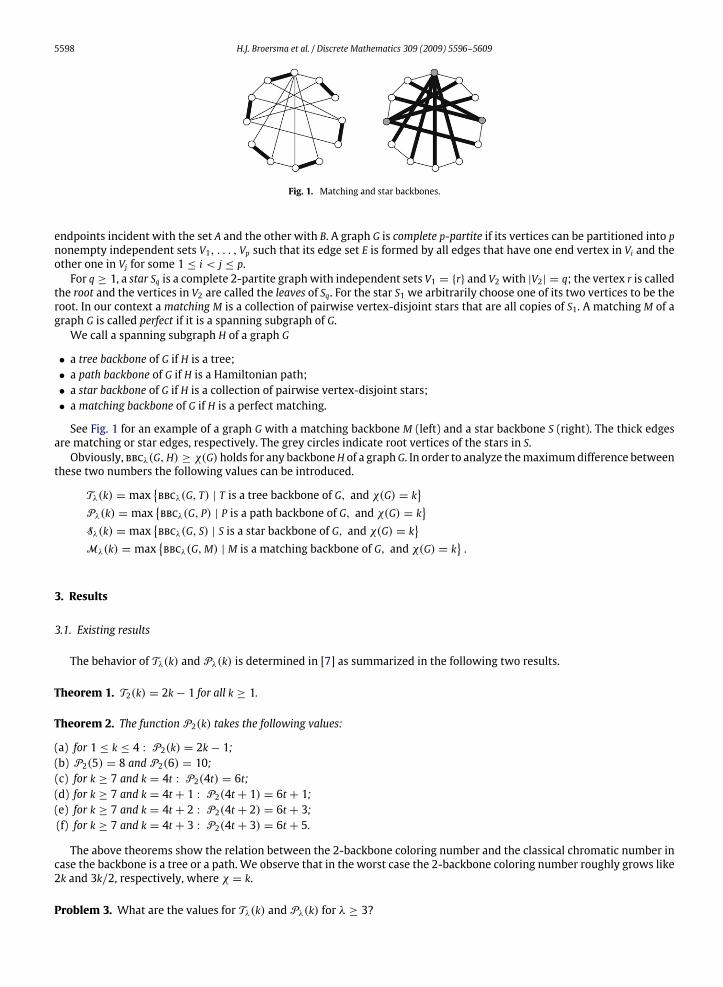
Fig. 2. The graph T(9, 3) with star backbone S.

We will show that these k color sets satisfy the conditions of Lemma 7. If j = s(λ − 1) + t for some integers s ≥ 0 and0 ≤ t ≤ λ−2, then d jλ

λ−1 e is equal to sλ in case t = 0 and to sλ+t+1 in case t > 0. Then Ci∩Dj is empty for all 1 ≤ i ≤ b kλc and

1 ≤ j ≤ b kλc(λ−1). Hence the k color sets as defined above are pairwise disjoint, and cover the whole range 1, . . . , 2k−b k

λc.

We observe that two colors ai, aj in two different sets Ci and Cj are at least λ apart from each other. We define bj := j+ kfor 1 ≤ j ≤ k− b k

λc. The smallest gap between a color bj and a color ai is 1+ k− ((b k

λc − 1)λ+ 1) = k− b k

λcλ+ λ ≥ λ.

For j = 1, . . . , b kλc(λ− 1), the distance between two colors in a color set Dj is

j+ k−⌈

jλ

λ− 1

⌉= j+ k−

⌈j+

j

λ− 1

⌉= k−

⌈j

λ− 1

⌉≥ k−

⌈b

kλc(λ− 1)

λ− 1

⌉= k−

⌊k

λ

⌋.

Also the distance between two colors in a color set Dj for j = b kλc(λ− 1)+ 1, . . . , k−b k

λc is at least k−b k

λc. We deduce that

k−⌊k

λ

⌋=

⌈k(λ− 1)

λ

⌉≥

⌈(2λ+ 1)(λ− 1)

λ

⌉=

⌈2λ− 1−

1λ

⌉= 2λ− 1.

Hence, all conditions of Lemma 7 are satisfied. This implies that (G, S) has a λ-backbone (2k− b kλc)-coloring.

5.2. Proof of the lower bounds

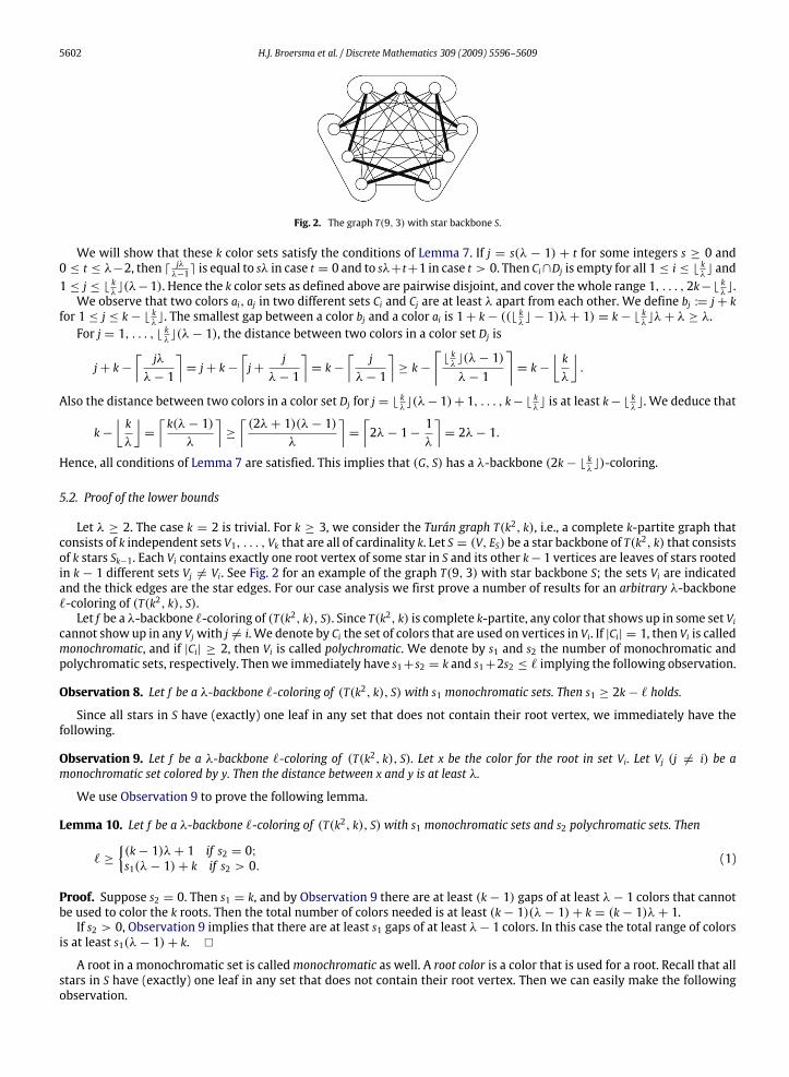
Let λ ≥ 2. The case k = 2 is trivial. For k ≥ 3, we consider the Turán graph T(k2, k), i.e., a complete k-partite graph thatconsists of k independent sets V1, . . . , Vk that are all of cardinality k. Let S = (V, ES) be a star backbone of T(k2, k) that consistsof k stars Sk−1. Each Vi contains exactly one root vertex of some star in S and its other k− 1 vertices are leaves of stars rootedin k − 1 different sets Vj 6= Vi. See Fig. 2 for an example of the graph T(9, 3) with star backbone S; the sets Vi are indicatedand the thick edges are the star edges. For our case analysis we first prove a number of results for an arbitrary λ-backbone`-coloring of (T(k2, k), S).

Let f be a λ-backbone `-coloring of (T(k2, k), S). Since T(k2, k) is complete k-partite, any color that shows up in some set Vi

cannot show up in any Vj with j 6= i. We denote by Ci the set of colors that are used on vertices in Vi. If |Ci| = 1, then Vi is calledmonochromatic, and if |Ci| ≥ 2, then Vi is called polychromatic. We denote by s1 and s2 the number of monochromatic andpolychromatic sets, respectively. Then we immediately have s1+ s2 = k and s1+2s2 ≤ ` implying the following observation.

Observation 8. Let f be a λ-backbone `-coloring of (T(k2, k), S) with s1 monochromatic sets. Then s1 ≥ 2k− ` holds.

Since all stars in S have (exactly) one leaf in any set that does not contain their root vertex, we immediately have thefollowing.

Observation 9. Let f be a λ-backbone `-coloring of (T(k2, k), S). Let x be the color for the root in set Vi. Let Vj (j 6= i) be amonochromatic set colored by y. Then the distance between x and y is at least λ.

We use Observation 9 to prove the following lemma.

Lemma 10. Let f be a λ-backbone `-coloring of (T(k2, k), S) with s1 monochromatic sets and s2 polychromatic sets. Then

` ≥

{(k− 1)λ+ 1 if s2 = 0;s1(λ− 1)+ k if s2 > 0.

(1)

Proof. Suppose s2 = 0. Then s1 = k, and by Observation 9 there are at least (k− 1) gaps of at least λ− 1 colors that cannotbe used to color the k roots. Then the total number of colors needed is at least (k− 1)(λ− 1)+ k = (k− 1)λ+ 1.

If s2 > 0, Observation 9 implies that there are at least s1 gaps of at least λ− 1 colors. In this case the total range of colorsis at least s1(λ− 1)+ k. �

A root in a monochromatic set is called monochromatic as well. A root color is a color that is used for a root. Recall that allstars in S have (exactly) one leaf in any set that does not contain their root vertex. Then we can easily make the followingobservation.

H.J. Broersma et al. / Discrete Mathematics 309 (2009) 5596–5609 5603

Observation 11. Let f be a λ-backbone `-coloring of (T(k2, k), S). Let x be the color for the root in Vi. Then there are (at least)k− 1 different colors y1, . . . , yi−1, yi+1, . . . , yk that have distance at least λ to x: every Vj (j 6= i) contains a vertex with color yj.

Due to Observation 11 we can prove the following lemma.

Lemma 12. Let f be a λ-backbone `-coloring of (T(k2, k), S). If ` ≤ k+2λ−3, then only colors from A = {1, . . . , `− k−λ+2}and B = {k+ λ− 1, . . . , `} can be assigned to root vertices.

Proof. Suppose a root v is assigned color c with c in {` − k − λ + 3, . . . , k + λ − 2}. By Observation 11 there have to be atleast k − 1 colors with distance at least λ from c. If λ + 1 ≤ c ≤ ` − λ, only colors in {1, . . . , c − λ} and in {c + λ, . . . , `}can be used. These sets together contain c − λ + ` − (c + λ) + 1 = ` − 2λ + 1 ≤ k − 2 colors. Hence either c ≤ λ orc ≥ ` − λ + 1 holds. If c ≤ λ, then only colors in {c + λ, . . . , `} are at distance at least λ. The cardinality of this set is`− (c+ λ)+ 1 ≤ `− (`− k− λ+ 3)− λ+ 1 = k− 2. If c ≥ `− λ+ 1, then only colors in {1, . . . , c− λ} are at distance atleast λ. The cardinality of this set is c− λ ≤ k+ λ− 2− λ = k− 2. �

We are now ready to make our case analysis.Case (b) 3 ≤ k ≤ 2λ− 3.

Suppose there exists a λ-backbone `-coloring of (T(k2, k), S) with ` = d 3k2 e + λ − 3 colors. Then ` = d 3k

2 e + λ − 3 ≤k+d k2 e+λ−3 ≤ k+2λ−3 and by Lemma 12 only colors in A = {1, . . . , d k2 e−1} and colors in B = {k+λ−1, . . . , d 3k

2 e+λ−3}can be used on roots. Each root is in a different independent set Vi. Therefore the number of different root colors is equal tok. However, the total number of colors in A united with B is 2(d k2 e − 1) < k. This contradiction shows that we must have` ≥ d 3k

2 e + λ− 2.Case (c, d) 2λ− 1 ≤ k ≤ 2λwith λ = 2 or 2λ− 2 ≤ k ≤ 2λ− 1 with λ ≥ 3.

Suppose there exists a λ-backbone `-coloring of (T(k2, k), S) with ` = k + 2λ − 3 colors. By Lemma 12, only colors inA = {1, . . . ,λ− 1} and B = {k+ λ− 1, . . . , k+ 2λ− 3}may be used on roots. By Observation 8, s1 ≥ 2k− ` = k− 2λ+ 3 ≥2λ− 2− 2λ+ 3 ≥ 1. So there exists at least one monochromatic set. Let y be the (root) color used on this set. Without lossof generality we may assume that y is in A. By Observation 9, all other k − 1 root colors must be in B. However, B containsλ− 1 < k− 1 colors. This contradiction shows that we must have ` ≥ k+ 2λ− 2.Case (e) k = 2λwith λ ≥ 3.

Suppose there exists a λ-backbone `-coloring of (T(k2, k), S) with 2k− 2 = 4λ− 2 colors. If s2 = 0, then by (1) we wouldhave 2k− 2 = ` ≥ (k− 1)λ+ 1 ≥ 3(k− 1)+ 1 = 3k− 2. Hence s2 > 0.

By Observation 8, s1 ≥ 2k− ` = 2. Together with (1) we then deduce that

4λ− 2 = ` ≥ s1(λ− 1)+ k ≥ 2(λ− 1)+ 2λ = 4λ− 2.

Hence we find that s1 = 2, and ` = s1(λ − 1) + k. Due to Observation 9, there are only three feasible ways to choose kdifferent root colors:

1. monochromatic roots: 1,λ+ 1, other roots: 2λ+ 1, . . . , 4λ− 2;2. monochromatic roots: 1, 4λ− 2, other roots: λ+ 1, . . . , 3λ− 2;3. monochromatic roots: 3λ− 2, 4λ− 2, other roots: 1, . . . , 2λ− 2.

Consider situation 1. Since color 2λ+ 1 is a root color, by Observation 11, in every other color set there must be at leastone color that has distance at least λ to color 2λ+ 1. This necessary condition is already met for the sets with root color 1,root color λ + 1 or root colors 3λ + 1, . . . , 4λ − 2. However, the sets with root colors 2λ + 2, . . . , 3λ need an extra color.Hence, we need λ− 1 extra colors that have distance at least λ to color 2λ+ 1. There are exactly λ− 1 such colors available,namely colors 2, . . . ,λ. So one of the colors 2, . . . ,λmust be in the same set with color 2λ+ 2.

Simultaneously, since color 2λ + 2 is also a root color, in every other color set there must be at least one color thathas distance at least λ to color 2λ + 2. This condition is not met yet for the sets with root color 2λ + 1 or root colors2λ + 3, . . . , 3λ + 1. To satisfy the condition, we need λ extra colors that have distance at least λ to color 2λ + 2. The onlyavailable colors are colors 2, . . . ,λ and color λ+ 2. This implies that none of the colors 2, . . . ,λ can be in the same set withcolor 2λ+ 2. This contradiction shows that we must have ` ≥ 2k− 1.

Consider situation 2. Since color λ + 1 is a root color, by Observation 11, in every other color set there must be at leastone color that has distance at least λ to color λ + 1. This necessary condition is already met for the sets with root color 1,root color 4λ − 2 or root colors 2λ + 1, . . . , 3λ − 2. However, the sets with root colors λ + 2, . . . , 2λ need an extra color.Hence, we need λ− 1 extra colors that have distance at least λ to color λ+ 1. There are exactly λ− 1 such colors available,namely colors 3λ− 1, . . . , 4λ− 3. So one of the colors 3λ− 1, . . . , 4λ− 3 must be in the same set with color λ+ 2.

Simultaneously, since color λ + 2 is also a root color, in every other color set there must be at least one color that hasdistance at least λ to color λ+2. This condition is not met yet for the sets with root color λ+1 or root colors λ+3, . . . , 2λ+1.To satisfy the condition, we need λ extra colors that have distance at least λ to color λ+2. The only available colors are color2 and the colors 3λ−1, . . . , 4λ−3. This implies that none of the colors 3λ−1, . . . , 4λ−3 can be in the same set with colorλ+ 2. This contradiction shows that we must have ` ≥ 2k− 1.

5604 H.J. Broersma et al. / Discrete Mathematics 309 (2009) 5596–5609

By symmetry, situation 3 yields the same conclusion as situation 1. Hence, we conclude that any λ-backbone `-coloringof (T(k2, k), S) has ` ≥ 2k− 1.

Case (f) k ≥ 2λ+ 1.Suppose there exists a λ-backbone `-coloring of (T(k2, k), S) with ` = 2k − b k

λc − 1 colors. Suppose s2 = 0. Then there

are only monochromatic sets, i.e., s1 = k. By (1) the total number of colors needed is at least (k − 1)λ + 1. However, thedifference between this number and ` is

(k− 1)λ+ 1−(

2k−⌊k

λ

⌋− 1

)= k(λ− 2)+

⌊k

λ

⌋− λ+ 2 ≥ 2λ2

− 4λ+ 2 > 0.

Hence s2 > 0. Write k = aλ + r for some integers a ≥ 2 and 0 ≤ r ≤ λ − 1. By Observation 8, s1 ≥ 2k − ` = b kλc + 1

holds. Together with (1) this implies that we need at least (b kλc+1)(λ−1)+ k colors. However, the difference between this

number and ` is (b kλc + 1)(λ− 1)+ k− (2k− b k

λc − 1) = b k

λcλ+ λ− k = λ− r > 0. This contradiction shows that we must

have ` ≥ 2k− b kλc.

This finishes the proof of the lower bounds, and we have completed the proof of Theorem 4.

6. Proof of Theorem 5

We prove Theorem 5 in two steps. First we show that bbcλ(G,M) for any graph G with arbitrary matching backbone M isat most the value of Mλ(χ(G)) as given in Theorem 5. Next we present a class of graphs G that have a matching backbone Msuch that bbcλ(G,M) is at least the value of Mλ(χ(G)) that is given in Theorem 5. This way we obtain coinciding upper andlower bounds on Mλ(k) proving the theorem.

6.1. Proof of the upper bounds

Let G = (V, E) be a graph with χ(G) = k and let V1, . . . , Vk denote the corresponding independent sets in a k-coloring. LetM = (V, EM) be a matching backbone of G.

Case (a) 2 ≤ k ≤ λ.If k = 2 then G is bipartite, and we use colors 1 and λ + 1. Let k ≥ 3. Let uv be a matching edge with u ∈ Vi and v ∈ Vj

for some 1 ≤ i < j ≤ k. We color u by i and v by λ+ j− 1. Then the difference between the colors of u and v is at least λ. Sovertices in V1 get color 1, vertices in Vi with 2 ≤ i ≤ k− 1 get color i or λ+ i− 1, and vertices in Vk get color λ+ k− 1. Hence,we have obtained a λ-backbone (λ+ k− 1)-coloring of (G,M).

Case (b) λ+ 1 ≤ k ≤ 2λ.Let uv be a matching edge with u ∈ Vi and v ∈ Vj for some 1 ≤ i < j ≤ k. We color u by i and v by k + j − 2. This way we

obtain a λ-backbone (2k− 2)-coloring of (G,M).For the cases (c)–(f) we need the following lemma. Observe that this lemma is exactly the same as Lemma 7 except that

condition (vi) of Lemma 7 could be dropped. The first two paragraphs of the proof can be copied from the proof of Lemma 7.

Lemma 13. Let G = (V, E) be a graph withχ(G) = k and let V1, . . . , Vk denote the corresponding independent sets in a k-coloring.Let M = (V, EM) be a matching backbone of G. For i = 1, . . . , p, let Ci = {ai} be a set consisting of one color. For j = 1, . . . , q,let Dj = {bj, cj} be a set consisting of two colors. Let d = max{a1, . . . , ap, b1, . . . , bq, c1, . . . , cq}. Then (G,M) has a λ-backboned-coloring if the following conditions are satisfied:

(i) p+ q = k.(ii) Ci ∩ Cj = ∅ for all 1 ≤ i < j ≤ p.

(iii) Di ∩ Dj = ∅ for all 1 ≤ i < j ≤ q.(iv) Ci ∩ Dj = ∅ for all 1 ≤ i ≤ p and 1 ≤ j ≤ q.(v) |ai − aj| ≥ λ for all 1 ≤ i < j ≤ p.

(vi) |bj − cj| ≥ 2λ− 1 for all 1 ≤ j ≤ q.

Proof. Let uv be a matching edge, where u ∈ Vi with 1 ≤ i ≤ p, and v ∈ Vj with p+ 1 ≤ j ≤ k. Then u has color ai. Then colorsai − λ+ 1, . . . , ai + λ− 1 are forbidden colors for v. The distance between ai + λ− 1 and ai − λ+ 1 is 2λ− 2. Since the twocolors in Dj−p have pairwise distance at least 2λ− 1 due to (vi), at least one of them is feasible for v.

For all matching edges uv with u ∈ Vi and v ∈ Vj for some p + 1 ≤ i < j ≤ k we choose u to be the root. We color u withbi. The remaining vertices, whose colors have not yet been fixed, are all leaf vertices in sets Vj with p+ 1 ≤ j ≤ k. Again dueto (vi) we can color them with a feasible color from Dj−p. This finishes the proof of the lemma. �

Below we show which color sets we use for each case. To check that these color sets satisfy the conditions of Lemma 13is a simple exercise and left to the reader.

H.J. Broersma et al. / Discrete Mathematics 309 (2009) 5596–5609 5605

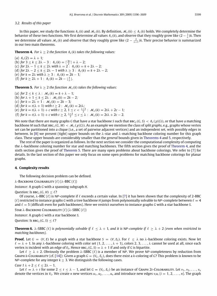
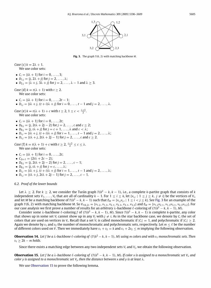
Fig. 3. The graph T(6, 2) with matching backbone M.

Case (c) k = 2λ+ 1.We use color sets:

• Ci = {iλ+ 1} for i = 0, . . . , 3;• D1,j = {j, 2λ+ j} for j = 2, . . . ,λ;• D2,j = {λ+ j, 3λ+ j} for j = 2, . . . ,λ− 1 and λ ≥ 3.

Case (d) k = t(λ+ 1) with t ≥ 2.We use color sets:

• Ci = {iλ+ 1} for i = 0, . . . , 2t − 1;• Di,j = {iλ+ j, (t + i)λ+ j} for i = 0, . . . , t − 1 and j = 2, . . . ,λ.

Case (e) k = t(λ+ 1)+ c with t ≥ 2, 1 ≤ c < λ+32 .

We use color sets:

• Ci = {iλ+ 1} for i = 0, . . . , 2t;• D0,j = {j, 2tλ+ 2j− 2} for j = 2, . . . , c and c ≥ 2;• D0,j = {j, tλ+ j} for j = c+ 1, . . . ,λ and c < λ;• Di,j = {iλ+ j, (t + i)λ+ j} for i = 1, . . . , t − 1 and j = 2, . . . ,λ;• Dt,j = {tλ+ j, 2tλ+ 2j− 1} for j = 2, . . . , c and c ≥ 2.

Case (f) k = t(λ+ 1)+ c with t ≥ 2, λ+32 ≤ c ≤ λ.

We use color sets:

• Ci = {iλ+ 1} for i = 0, . . . , 2t;• C2t+1 = {2tλ+ 2c− 2};• D0,j = {j, 2tλ+ 2j− 2} for j = 2, . . . , c− 1;• D0,j = {j, tλ+ j} for j = c, . . . ,λ;• Di,j = {iλ+ j, (t + i)λ+ j} for i = 1, . . . , t − 1 and j = 2, . . . ,λ;• Dt,j = {tλ+ j, 2tλ+ 2j− 1} for j = 2, . . . , c− 1.

6.2. Proof of the lower bounds

Let λ ≥ 2. For k ≥ 2, we consider the Turán graph T(k2− k, k − 1), i.e., a complete k-partite graph that consists of k

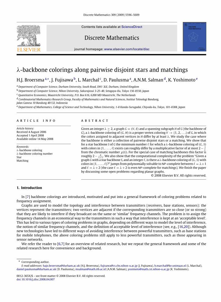
independent sets V1, . . . , Vk that are all of cardinality k − 1. For 1 ≤ i ≤ k, let {vi,j | 1 ≤ j ≤ k, j 6= i} be the vertices of Vi,and let M be a matching backbone of T(k2

− k, k− 1) such that EM = {vi,jvj,i | 1 ≤ i < j ≤ k}. See Fig. 3 for an example of thegraph T(6, 2) with matching backbone M. So VT(6,2) = {v1,2, v1,3, v2,1, v2,3, v3,1, v3,2} and EM = {v1,2v2,1, v1,3v3,1, v2,3v3,2}. Forour case analysis we first prove a number of results for an arbitrary λ-backbone `-coloring of (T(k2

− k, k− 1),M).Consider some λ-backbone `-coloring f of (T(k2

− k, k − 1),M). Since T(k2− k, k − 1) is complete k-partite, any color

that shows up in some set Vi cannot show up in any Vj with j 6= i. As in the star backbone case, we denote by Ci the set ofcolors that are used on vertices in Vi. Recall that a set Vi is called monochromatic if |Ci| = 1, and polychromatic if |Ci| ≥ 2.Again we denote by s1 and s2 the number of monochromatic and polychromatic sets, respectively. Let m ≤ ` be the numberof different colors used on V . Then we immediately have s1 + s2 = k and s1 + 2s2 ≤ m implying the following observation.

Observation 14. Let f be a λ-backbone `-coloring of (T(k2− k, k− 1),M) using m colors and with s1 monochromatic sets. Then

s1 ≥ 2k− m holds.

Since there exists a matching edge between any two independent sets Vi and Vj, we obtain the following observation.

Observation 15. Let f be a λ-backbone `-coloring of (T(k2− k, k− 1),M). If color x is assigned to a monochromatic set Vi, and

color y is assigned to a monochromatic set Vj, then the distance between x and y is at least λ.

We use Observation 15 to prove the following lemma.

5606 H.J. Broersma et al. / Discrete Mathematics 309 (2009) 5596–5609

Lemma 16. Let f be a λ-backbone `-coloring of (T(k2− k, k− 1),M). Then

` ≥2λkλ+ 1

−λ− 1λ+ 1

. (2)

Proof. Let m be the number of different colors that f uses. Observation 15 yields ` ≥ λ(s1 − 1) + 1. Together withObservation 14 and m ≤ `, we obtain ` ≥ λ(s1 − 1) + 1 ≥ λ(2k − m − 1) + 1 ≥ λ(2k − ` − 1) + 1, which is equivalent toinequality (2). �

Also the following lemma is useful.

Lemma 17. Let f be a λ-backbone `-coloring of (T(k2− k, k − 1),M). If ` ≤ k + 2λ − 3 then only colors from A =

{1, . . . , `− k− λ+ 2} and B = {k+ λ− 1, . . . , `} can be assigned to monochromatic sets.

Proof. Suppose a vertex v from a monochromatic set is assigned color c with c in {` − k − λ + 3, . . . , k + λ − 2}. Recallthat there exists a matching edge between any two independent sets Vi and Vj. Then there are at least k − 1 colorsthat have distance at least λ to c. If λ + 1 ≤ c ≤ ` − λ, only colors in {1, . . . , c − λ} and in {c + λ, . . . , `} can beused. These sets together contain c − λ + ` − (c + λ) + 1 = ` − 2λ + 1 ≤ k − 2 colors. Hence either c ≤ λ orc ≥ ` − λ + 1 holds. If c ≤ λ, then only colors in {c + λ, . . . , `} are at distance at least λ. The cardinality of this set is`− (c+ λ)+ 1 ≤ `− (`− k− λ+ 3)− λ+ 1 = k− 2. If c ≥ `− λ+ 1, then only colors in {1, . . . , c− λ} are at distance atleast λ. The cardinality of this set is c− λ ≤ k+ λ− 2− λ = k− 2. �

We are now ready to make our case analysis.Case (a) 2 ≤ k ≤ λ.

The case k = 2 is trivial. Let k ≥ 3. Suppose (T(k2− k, k− 1),M) has a λ-backbone `-coloring with ` = k+ λ− 2 colors.

By Lemma 17, we find that s1 = 0. Colors k− 1, . . . ,λ cannot be used at all, since there is no color in {1, . . . ,λ+ k− 2} thathas distance at least λ to one of them. So we can only use colors in {1, . . . , k− 2} and {λ+ 1, . . . ,λ+ k− 2}. Then the totalnumber m of different colors is at most 2(k− 2). Hence, by Observation 14 we find that s1 ≥ 2k−m > 0. This contradictionshows that we must have ` ≥ k+ λ− 1.Case (b) λ+ 1 ≤ k ≤ 2λ.

Suppose (T(k2− k, k − 1),M) has a λ-backbone `-coloring with ` = 2k − 3 colors. By Observation 14, we find that

s1 ≥ 2k − m ≥ 2k − ` ≥ 3 must hold. By Lemma 17, only monochromatic colors in A = {1, . . . , k − λ − 1} andB = {k + λ − 1, . . . , 2k − 3} can be used. Both sets have k − λ − 1 ≤ λ − 1 elements. Then, by Observation 15, at mostone color in A and at most one color in B can be used for monochromatic sets. Hence we find that s1 ≤ 2. This contradictionshows that ` ≥ 2k− 2.Case (c) k = 2λ+ 1.

Analogously to the proof of the previous case we can show that ` ≥ 2k − 3 must hold for any λ-backbone `-coloring of(T(k2

− k, k− 1),M).Case (d) k = t(λ+ 1) with t ≥ 2.

Inequality (2) yields ` ≥ 2tλ− λ−1λ+1 = 2tλ− 1+ 2

λ+1 for any λ-backbone `-coloring of (T(k2− k, k− 1),M). Since ` is an

integer, this implies that ` ≥ 2tλ.Case (e) k = t(λ+ 1)+ c with t ≥ 2 and 1 ≤ c < λ+3

2 .Inequality (2) yields ` ≥ 2tλ+ 2λc

λ+1 −λ−1λ+1 = 2tλ+2c−1+ 2−2c

λ+1 > 2tλ+2c−1+ 2−λ−3λ+1 = 2tλ+2c−2 for any λ-backbone

`-coloring of (T(k2− k, k− 1),M). Since ` is an integer, we have found that ` ≥ 2tλ+ 2c− 1.

Case (f) k = t(λ+ 1)+ c with t ≥ 2 and λ+32 ≤ c ≤ λ.

Inequality (2) yields ` ≥ 2tλ + 2λcλ+1 −

λ−1λ+1 = 2tλ + 2c − 1 + 2−2c

λ+1 ≥ 2tλ + 2c − 1 + 2−2λλ+1 = 2tλ + 2c − 3 + 2

λ+1 for anyλ-backbone `-coloring of (T(k2

− k, k− 1),M). Since ` is an integer, this implies that ` ≥ 2tλ+ 2c− 2.This finishes the proof of the lower bounds, and we have completed the proof of Theorem 5.

7. Matching backbones for planar graphs

7.1. Implications of the four color theorem

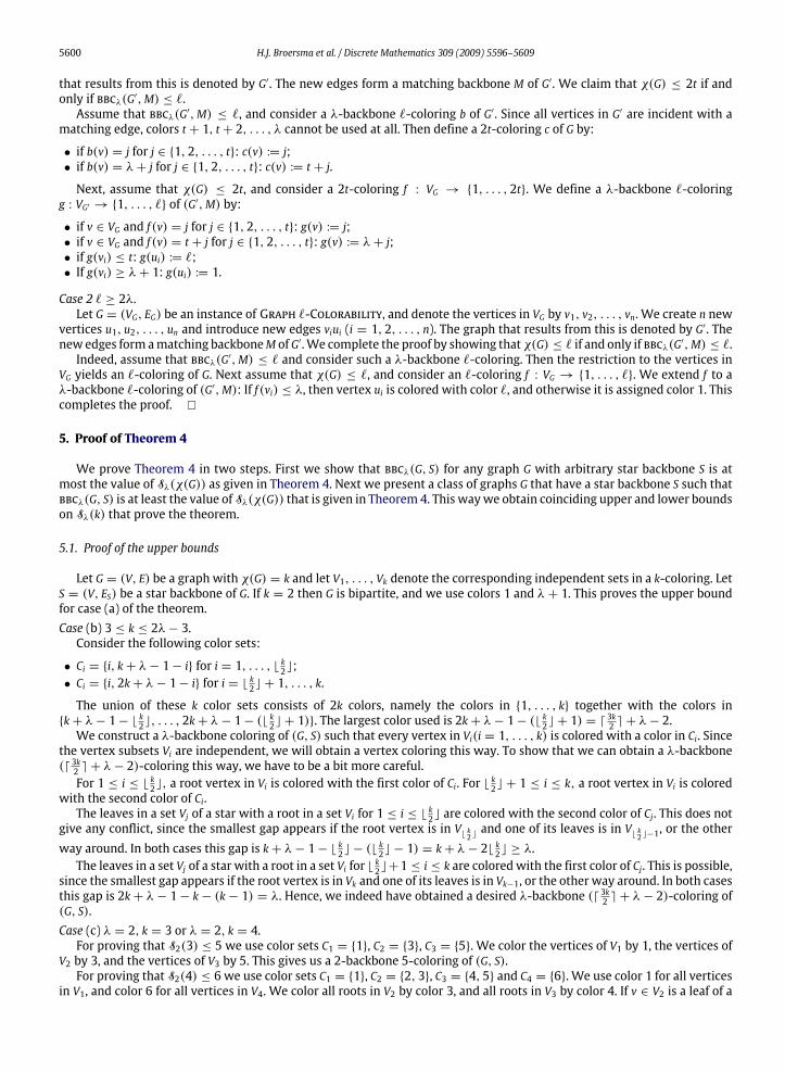
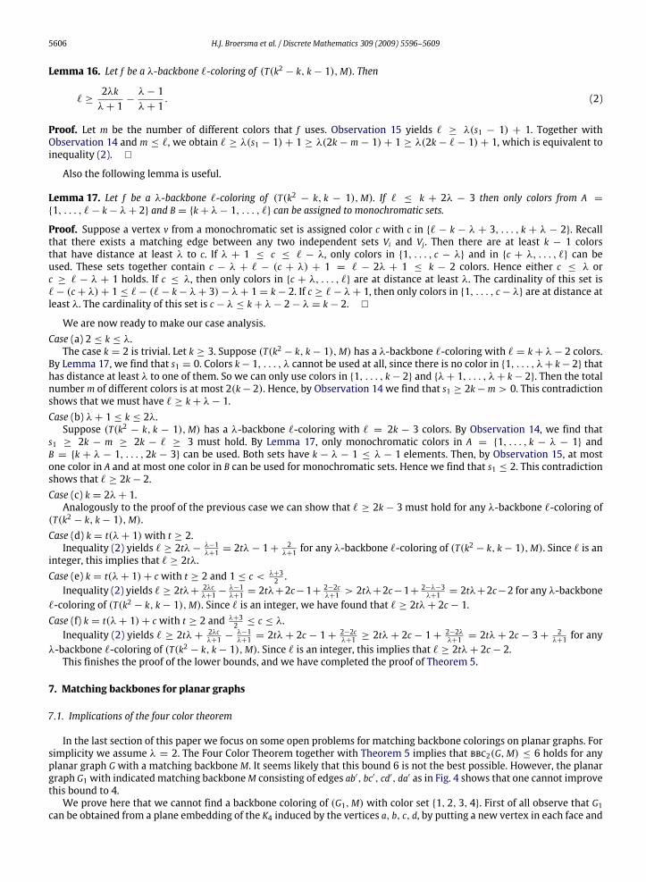
In the last section of this paper we focus on some open problems for matching backbone colorings on planar graphs. Forsimplicity we assume λ = 2. The Four Color Theorem together with Theorem 5 implies that bbc2(G,M) ≤ 6 holds for anyplanar graph G with a matching backbone M. It seems likely that this bound 6 is not the best possible. However, the planargraph G1 with indicated matching backbone M consisting of edges ab′, bc′, cd′, da′ as in Fig. 4 shows that one cannot improvethis bound to 4.

We prove here that we cannot find a backbone coloring of (G1,M) with color set {1, 2, 3, 4}. First of all observe that G1can be obtained from a plane embedding of the K4 induced by the vertices a, b, c, d, by putting a new vertex in each face and

H.J. Broersma et al. / Discrete Mathematics 309 (2009) 5596–5609 5607

Fig. 4. A graph G1 with a matching backbone M such that bbc2(G1,M) = 5.

adding edges from this new vertex to the three vertices on the boundary of the face, and assigning the label x′ to the newvertex in the triangular face bounded by the cycle uvwu, where {u, v,w, x} = {a, b, c, d}. Suppose we only use colors 1, 2, 3, 4.Then it is clear from this construction that a, b, c and d get different colors, and that the colors of a vertex and its primedcounterpart are the same. Without loss of generality assume that a and a′ get color 2. Then both b′ and d must get color 4, acontradiction. It is routine to check that bbc2(G1,M) = 5.

The following problems are still open.

Problem 18. Is bbc2(G,M) ≤ 5 for any planar graph G with a matching backbone M?

Problem 19. Is there a proof of bbc2(G,M) ≤ 6 that does not require the Four Color Theorem?

7.2. Cyclic backbone colorings

In the last part of this section we introduce a special kind of 2-backbone coloring with a cyclic property as defined below.Our motivation for doing this is to get a better understanding of the structure of the original (acyclic) 2-matching backbonecolorings of planar graphs. We prove a sharp result with respect to the upper bound on the number of colors needed to colorplanar graphs in the way explained below.

Let H = (V, EH) be a backbone of the graph G = (V, EG). A 2-backbone coloring f : V → {1, . . . , `} of (G,H) is called an`-cyclic 2-backbone coloring of (G,H), if no edge of EH joins two vertices with color 1 and color ` in V . In a 2-backbone coloringwe say that two colors x and y are adjacent if |x−y| ≤ 1. In an `-cyclic 2-backbone coloring we also say that color 1 and color` are adjacent.

The study of cyclic colorings in the context of frequency assignment is well motivated in [17].For the proof of Theorem 21 we first construct the following useful gadget.

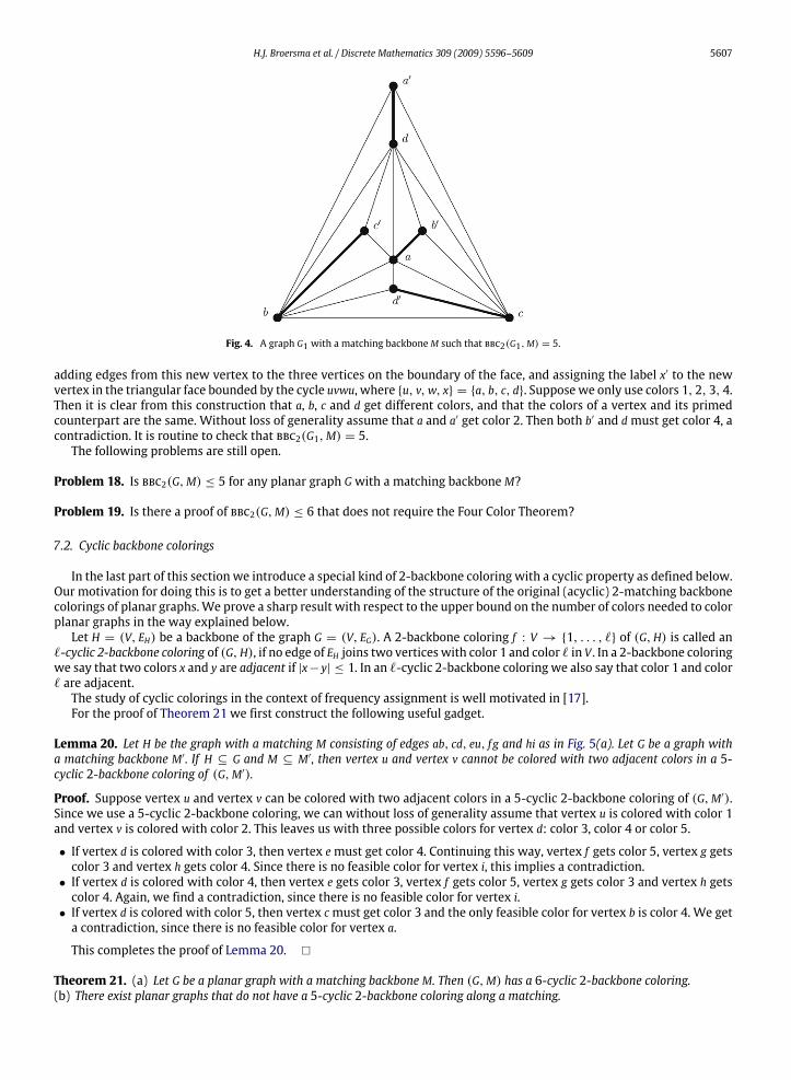
Lemma 20. Let H be the graph with a matching M consisting of edges ab, cd, eu, f g and hi as in Fig. 5(a). Let G be a graph witha matching backbone M′. If H ⊆ G and M ⊆ M′, then vertex u and vertex v cannot be colored with two adjacent colors in a 5-cyclic 2-backbone coloring of (G,M′).

Proof. Suppose vertex u and vertex v can be colored with two adjacent colors in a 5-cyclic 2-backbone coloring of (G,M′).Since we use a 5-cyclic 2-backbone coloring, we can without loss of generality assume that vertex u is colored with color 1and vertex v is colored with color 2. This leaves us with three possible colors for vertex d: color 3, color 4 or color 5.

• If vertex d is colored with color 3, then vertex e must get color 4. Continuing this way, vertex f gets color 5, vertex g getscolor 3 and vertex h gets color 4. Since there is no feasible color for vertex i, this implies a contradiction.• If vertex d is colored with color 4, then vertex e gets color 3, vertex f gets color 5, vertex g gets color 3 and vertex h gets

color 4. Again, we find a contradiction, since there is no feasible color for vertex i.• If vertex d is colored with color 5, then vertex c must get color 3 and the only feasible color for vertex b is color 4. We get

a contradiction, since there is no feasible color for vertex a.

This completes the proof of Lemma 20. �

Theorem 21. (a) Let G be a planar graph with a matching backbone M. Then (G,M) has a 6-cyclic 2-backbone coloring.(b) There exist planar graphs that do not have a 5-cyclic 2-backbone coloring along a matching.

5608 H.J. Broersma et al. / Discrete Mathematics 309 (2009) 5596–5609

(a) Graph H with matching M. (b) Planar graph G2 .

Fig. 5.

Proof. (a) By the Four Color Theorem, we know that the chromatic number of a planar graph G is at most 4. For a vertex v inG, we denote by n(v) the only neighbor of v in M. We can construct a 6-cyclic 2-backbone coloring b of (G,M) by replacingthe colors of a 4-coloring c of G as follows:

• if c(v) = 1: b(v) := 1;• if c(v) = 2: b(v) := 3;• if c(v) = 3: b(v) := 5;• if c(v) = 4 and c(n(v)) = 1: b(v) := 4;• if c(v) = 4 and c(n(v)) = 2: b(v) := 6;• if c(v) = 4 and c(n(v)) = 3: b(v) := 2.

(b) We construct a planar graph G2 as follows. First we make three copies (H1,M1), (H2,M2), (H3,M3) of the pair (H,M)from Fig. 5(a), and glue them together at vertex v. Then we add one new vertex w and four new edges: the edge vw and theedges u1u2, u2u3 and u3u1 (see Fig. 5(b)). The vertex w and the edge vw are only added to guarantee that G2 has a perfectmatching. Let M′ be a matching backbone of G2 that contains all matchings Mi (i = 1, 2, 3) and the edge vw.

Suppose there exists a 5-cyclic 2-backbone coloring of (G2,M′). Without loss of generality we may assume that the vertexv is colored with color 1. Then, by Lemma 20, the vertices u1, u2 and u3 cannot be colored with colors 1, 2 and 5. On theother hand, u1, u2 and u3 must all get different colors, since they induce a K3. This contradiction completes the proof ofTheorem 21. �

Acknowledgments

We would like to thank the two anonymous referees for their useful feedback that helped in improving the presentationof our paper. The work of J.F. was partially supported by the 21st Century COE Program; Integrative Mathematical Sciences:Progress in Mathematics Motivated by Social and Natural Sciences.

References

[1] G. Agnarsson, M.M. Halldórsson, Coloring powers of planar graphs, SIAM J. Discrete Math. 16 (2003) 651–662.[2] H.L. Bodlaender, T. Kloks, R.B. Tan, J. van Leeuwen, λ-coloring of graphs, in: Proceedings of the 17th Annual Symposium on Theoretical Aspects of

Computer Science, STACS’2000, in: LNCS, vol. 1770, Springer, 2000, pp. 395–406.[3] J.A. Bondy, U.S.R. Murty, Graph Theory with Applications, Macmillan, London, 1976, Elsevier, New York.[4] O.V. Borodin, H.J. Broersma, A. Glebov, J. van den Heuvel, Stars and bunches in planar graphs. Part I: Triangulations, Diskretnyi Analiz i Issledovanie

Operatsii. Seriya 1 8 (2) (2001) 15–39. Preprint (2001) (in Russian).[5] O.V. Borodin, H.J. Broersma, A. Glebov, J. van den Heuvel, Stars and bunches in planar graphs. Part II: General planar graphs and colourings, Diskretnyi

Analiz i Issledovanie Operatsii. Seriya 1 8 (4) (2001) 9–33. Preprint (2001) (in Russian).[6] H.J. Broersma, A general framework for coloring problems: old results, new results and open problems, in: Proceedings of IJCCGGT 2003, in: LNCS,

vol. 3330, Springer, 2005, pp. 65–79.[7] H.J. Broersma, F.V. Fomin, P.A. Golovach, G.J. Woeginger, Backbone colorings for networks, in: Proceedings of WG 2003, in: LNCS, vol. 2880, Springer,

2003, pp. 131–142. The full paper version “Backbone colorings for graphs: tree and path backbones” has been published in J. Graph Theory 55 (2007)137–152. DOI link is: http://dx.doi.org/10.1002/jgt.20228.

[8] H.J. Broersma, L. Marchal, D. Paulusma, A.N.M. Salman, Improved upper bounds for λ-backbone colorings along matchings and stars, in: Proceedingsof SOFSEM 2007, in: Lecture Notes in Computer Science 4362, pp. 188–199, doi:10.1007/978-3-540-69507-3_15.

H.J. Broersma et al. / Discrete Mathematics 309 (2009) 5596–5609 5609

[9] G.J. Chang, D. Kuo, The L(2, 1)-labeling problem on graphs, SIAM J. Discrete Math. 9 (1996) 309–316.[10] J. Fiala, A.V. Fishkin, F.V. Fomin, Off-line and on-line distance constrained labeling of graphs, in: Proceedings of the 9th European Symposium on

Algorithms, ESA’2001, in: LNCS, vol. 2161, Springer, 2001, pp. 464–475.[11] J. Fiala, T. Kloks, J. Kratochvíl, Fixed-parameter complexity of λ-labelings, Discrete Appl. Math. 113 (2001) 59–72.[12] J. Fiala, J. Kratochvíl, A. Proskurowski, Distance constrained labelings of precolored trees, in: Proceedings of the 7th Italian Conference on Theoretical

Computer Science, ICTCS’2001, in: LNCS, vol. 2202, Springer, 2001, pp. 285–292.[13] D.A. Fotakis, S.E. Nikoletseas, V.G. Papadopoulou, P.G. Spirakis, Hardness results and efficient approximations for frequency assignment problems and

the radio coloring problem, Bull. Eur. Assoc. Theor. Comput. Sci. EATCS 75 (2001) 152–180.[14] M.R. Garey, D.S. Johnson, Computers and Intractability, A Guide to the Theory of NP-Completeness, W.H. Freeman and Company, New York, 1979.[15] J.R. Griggs, R.K. Yeh, Labelling graphs with a condition at distance 2, SIAM J. Discrete Math. 5 (1992) 586–595.[16] W.K. Hale, Frequency assignment: Theory and applications, Proc. IEEE 68 (1980) 1497–1514.[17] J. van den Heuvel, R.A. Leese, M.A. Shepherd, Graph labeling and radio channel assignment, J. Graph Theory 29 (1998) 263–283.[18] J. van den Heuvel, S. McGuinness, Colouring the square of a planar graph, J. Graph Theory 42 (2003) 110–124.[19] T.K. Jonas, Graph coloring analogues with a condition at distance two: L(2, 1)-labellings and list λ-labellings, Ph.D. Thesis, University of South Carolina

(1993).[20] R.A. Leese, Radio spectrum: A raw material for the telecommunications industry, in: Progress in Industrial Mathematics at ECMI 98, Teubner, Stuttgart,

1999, pp. 382–396.[21] M. Molloy, M.R. Salavatipour, A bound on the chromatic number of the square of a planar graph, J. Combin. Theory Ser. B 94 (2005) 189–213.