Download pdf - A POLYNOMIAL-TIME PRIMAL-DUAL AFFINE SCALING ALGORITHM …monteiro/publications/tech_reports/pd.pdf · determined by the current iterate is the weighted barrier path sp«;ified by

MATHEMATICS OF OPERATIONS RESEARCHVol. 15. No. 2. May 1>«»PriiileJ in U.S.A.

A POLYNOMIAL-TIME PRIMAL-DUAL AFFINE SCALINGALGORITHM FOR LINEAR AND CONVEX QUADRATICPROGRAMMING AND ITS POWER SERIES EXTENSION*^

RENATO D. C. MONTEIRO,* ILAN ADLER* ANDMAURICIO G. C. RESENDE**

We describe an algorithm for linear and convex quadratic programming problems that usespower series approximation of the weighted barrier path that passes throi^ the current iteratein order to find the next iterate. If r » 1 is the order of approximation used, we show that ouralgorithm has time complexity O(n'"""^'^*i."*'^'') iterations and O{n^ + n^r) arithmeticoperations per iteration, where n is the dimension of the problem and L is the size of the inputdata. When /• = 1, we show that the algorithm can be interpreted as an affine scaling algorithmin the primal-dual setup.

1. Introduction. After the presentation of the new polynomial-time algorithm forlinear programming by Karmarkar in his landmark paper [15], several so-callwi interiorpoint algorithms for linear and convex quadratic programming have been proposed.These algorithms can be classified into three main groups:

(a) Projective algorithms, e.g. [3], [4], [8], [14], [15], [29] and [34].(b) Affine scaling algorithms, originally proposed by Dikin [9]. See also [1], [5], [10]

and [33].(c) Path following algorithms, e.g. [13], [18], [19], [24], [25], [26], [28] and [32].

The algorithms of class (a) are known to have polynomial-time complexity requiringOinL) iterations. However, these methods appear not to perform well in practice [30].In contrast, the algorithms of group (b), while not known to have polynomial-timecomplexity, have exhibited good behavior on real world linear programs [1], [20], [23],[31]. Most path following algorithms of group (c) have been shown to require O(y^L)iterations. These algorithms use Newton's method to trace the path of minimizers forthe logarithmic barrier family of problems, the so-called central path. The Icârithmicbarrier function approach is usually attributed to Frisch [12] and is formally studied inFiacco and McCormick [11] in the context of nonlinear optimization. Continuoustrajectories for interior point methods were proposed by Karmarkar [16] and areextensively studied in Bayer and Lagarias [6] [7], Megiddo [21] and Megiddo and Shub[22]. Megiddo [21] related the central path to the classical barrier path in theframework of the primal-dual complementarity relationship. Kojima, Mizuno andYoshise [19] used this framework to describe a primal-dual interior point algorithmthat traces the central trajectory and has a woret time complexity of OinL) itraâtions.

•Received April 11,1988; revised Ctetober 20, 1988.AMS 1980 subject ctassificatim. Primary: 900)5; Sectmdary 90C25.lAOR I97S sidgect classificatim. Main: PKânnmng: Linear.OR/MS Index 1978 stdyect dasifkatim. Primary: 644 Pr<âniming/LMKar/AIgorithiBs/HUpsoidaL Sec-(»dary: 656 Pro^-aminiiig/N(Mlinear/c<»vex.Key words. Rxigramnui^. affine sc t f i^ power series extensifflis.^This research was partially funded by the United Stales Navy Office of Naval Reseaidi, undw contractMX»14-87-K-02)2 and Iqr the foaziUaa Pasâduate Edocation Aâcy—CATOS.* AT & T Bdl LAoMUjries.'University of CaBfomia, Beitatey.• •AT&T Ben U*ora«ories.

191

O364-765X/90/15O2/0191$01.25

192 RENATO D. C. MONTEIRO, ILAN ADLER & MAURICIO G. C. RESENDE

Monteiro and Adler [25] present a path following primal-dual algorithm that requiresOi'/nL) iterations.

This paper describes a modification of the algorithm of Montdro and Adler [25] andshows that the resulting algorithm can be interpreted as an affine scaling algorithm inthe primal-dual setting. We also show polynomial-time convergence for the primal-dualaffine scaling algorithm by using a readily available starting primal-dual solution lyingon the central path and a suitable fixed step size. Furthennore, we show finite globalconvergence (not necessarily polynomial) for any starting primal-dual solution. In [21]it is shown that there exists a path of minimizers for the we t ted barrier family ofproblems, that passes through any given primal-dual interior point. The directiongenerated by our primal-dual affine scaling algorithm is precisely the tangent vector tothe weighted barrier path at the current iterate. Hence, the infinitesimal trajectorydetermined by the current iterate is the weighted barrier path sp«;ified by this iterate.

We also present an algorithm bas«i on power series approximations of the weightedbarrier path that passes through the current iterate. We show that the complexity of thenumber of iterations is given by O(n^<iî/'>L<iî/'>) and that the work per iteration isOin^ + n^r) arithmetic operations, where r is the order of the power series approxi-mation used and L is the size of the problem. Hence, as r -^ oo, the number ofiterations required approaches Oi^nL). We develop this algorithm in the context ofconvex quadratic programming because it provides a more general setting and noadditional complication arises in doing so. We should mention that the idea of usinghigher order approximation by truncating power series is suggested in [17] and also ispresent in [1], [7] and [21]. However, no convergence analysis is discussed there.

The importance of starting the algorithm at a point close to the central path is alsoanalyzed. More specifically, the complexity of the number of iterations is given as afunction of the "distance" of the starting point to the central path. It should be not^that Megiddo and Shub [22] have analyzed how the starting point affects the behaviorof the continuous trajectory for the projective and affine scaUng algorithms.

This paper is organized as follows. In §2 we motivate the first order approximationalgorithm, by showing its relationship to the algorithm of Monteiro and Adler. We alsointerpret this first order approximation algorithm as an affine scaling algorithm in theprimal-dual setup. In §3 we present polynomial-time complexity results for theprimal-dual affine scaling algorithm (first order power series) in the context of linearprogramming and under the assumption that the starting point lies on the central path.In §4, we analyze the higher order approximation algorithm in the more generalcontext of convex quadratic programming. We also analyze how the choice for thestarting point affects the complexity of the number of iterations. Concluding remarksare made in §5.

2. MotivattoB. In this s«:tion we provide s(Hne motivation for ihs first orderversion of the algorithm that will be described in this p^Kx. We concentrate ourdiscussicm on the relatiraa^p betwmi this algraithm and the algorithm of Monteiroand Adler [25]. We also ve an interpretation of the first order algoritfim as an affinescaling algorithm in the primal-dual setup.

Throuût this p^per we adc^t the notation used in {191 a«l PS]. If the lower caseX = ixx,...,xj is an n-vector, then the corresponding upper case X deletes thediagonal matrix dia^x) = d i ^ X i , . . . , x J . We denote the j t h con^xHirait of ann-vector;t by X,, for; - ! , . . . , « . A p<Mnt(x, y, z) e « - x * « x ^ - will be <teaotedby ths lawet case w. Tlw kârithm of a i ^ numba: a > 0 on tttts natural base and onbase 2 will be denoted by In a and k ^ a respectivdy. We Aatote the 2.norm and theoo-norm in « " by |j • ft and |1 • «„ re^xxaivdy. FinaUy, far w - (x, y, z) e « " x ^ ^

POLYNOMUL-TIME PRIMAL-DUAl. AFFIME K : A U N G 193

X 91", we denote by /(w) = (/i(w),..., /.(w))^ e dt", the u-vector defined by

(1) /;(»v) = x,z,, i = \,...,n.

Consider the pair of the standard form linear program

(2) (P) minimize c^x

(3) subject to: Ax = b,

(4) x>Q,

and its dual

(5) (D) maximize fc'V

(6) subject to: A^y + z = c,

il) z>0,

where A is an m X n matrix, x, c and z are n-vectors and b and y are m-vectors. Weassume that the entries of A, b and c are integer.

We define the sets of interior feasible solutions of problems (P) and (D) as

(8) S= {xe^",Ax = b,x>0),

(9) T= {iy,z) e:^'"X^";A^y +z='c,z>0]

respojtively, and let

(10) W= {ix,y,z);xeS,iy,z)&T}.

We define the duaUty gap at a point w = (x, / , 2) e W as c^x - b^y. One can easilyverify that for any w B W, c'^x - b'^y = x^z. In view of this relation, we refer to theduality gap as the quantity JC'Z instead of the usual c^x - b^y. We make the followingassumptions regarding (P) and (D):

Assumption 2.1. ia) S * 0 .(b) r=?t 0 .(c) rank(v4) = m.Before we describe the primal-dual affine scaling algorithm, we briefly review the

concept of solution pathways for the wei^ted logarithmic barrier function family ofproblems associated with problem (P). For a comprehensive discussion of this subject,see [11] and [21].

TTie weighted barrier function method worics on a parametrized family of problemspenalized by the weighted barrier function as follows. The weighted barrfer functionproblem with parameter ji > 0 and weights Sj> 0, j = l,...,n is:

n

(11) (P^) minimize c x - p £ s hi Xj


(13) x>0.

194 RENATO D. C. MONTEIRO, ILAN ADLER & MAURIOO G. C. RESENDE

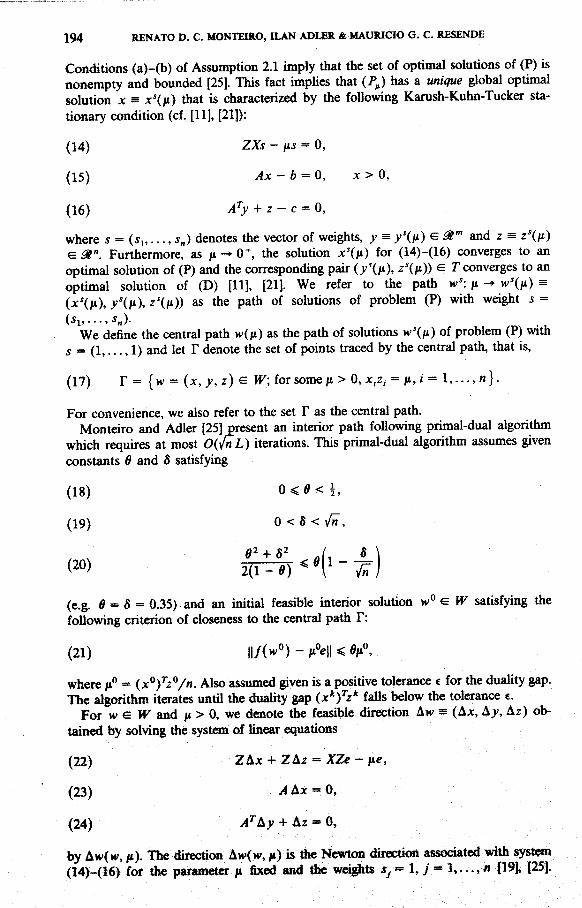
Conditions (a)-(b) of Assumption 2.1 imply that the set of optimal solutions of (P) isnonempty and bounded [25]. This fact implies that (P^) has a unique global optimalsolution X = x'ifi) that is characterized by the following Karush-Kuhn-Tucker sta-tionary condition (cf. [11], [21]):

(14) ZXs - M5 = 0,

(15) Ax-b = O, x>0,

(16)

where s = (s^,...,sj denotes the vector of weights, y = y'in) e ^ ' " and z = z'in)e ^" . Furthermore, as /x -• O"", the solution x'in) for (14)-(16) converges to anoptimal solution of (P) and the corresponding pair (y'in), z'in)) e r converges to anoptimal solution of (D) [11], [21]. We refer to the path w': (i -* w%n) =ix'in), y'ifi), z'in)) as the path of solutions of problem (P) with weight s =isi,..., sj.

We define the central path win) as the path of solutions w'(n) of problem (P) with,x = ( 1 , . . . , 1) and let T denote the set of points traced by the central path, that is,

(17) r = {w = ix,y,z) e W; for some > 0, JC,Z, = /i, J = 1, . . . , n} .

For convenience, we also refer to the set T as the central path.Monteiro and Adler [25] present an interior path following primal-dual algorithm

which requires at most Oii/nL) iterations. This primal-dual algorithm assumes givenconstants 6 and 8 satisfying

< I(18) 0 < fl < I,

(19) 0 < S <

(e.g. fl = 5 = 0.35) and an initial feasible interior solution w° & W satisfying thefollowing criterion of closeness to the central path F:

(21) Il/Cw") - All < 9yP,

where /i° = (x°)^2 "/"• Also assumed given is a positive tolerance « for the duality gap.The algorithm iterates until the duality gap (jc*)'z* falls below the tolerance e.

For w G W and ft > 0, we denote the feasible direction Aw (Ax, Aj, Az) ob-tained by solving the Systran of linear equations

(22) ZAx -I- ZAz = XZe - fie,

(23) ^ A x - 0 ,

(24) A^£iy + Az » 0,

by Aw(w, n). The direction Aw(w, ^) is flie Newton directitm associated with Systran(14)-(16) for the panmaeler n fixed and ê md^ts Sj = 1, / = 1,...,n {19J, [251-

POLYNOMIAL-TIME PRIMAL-DUAL AFFINE SCALING 195

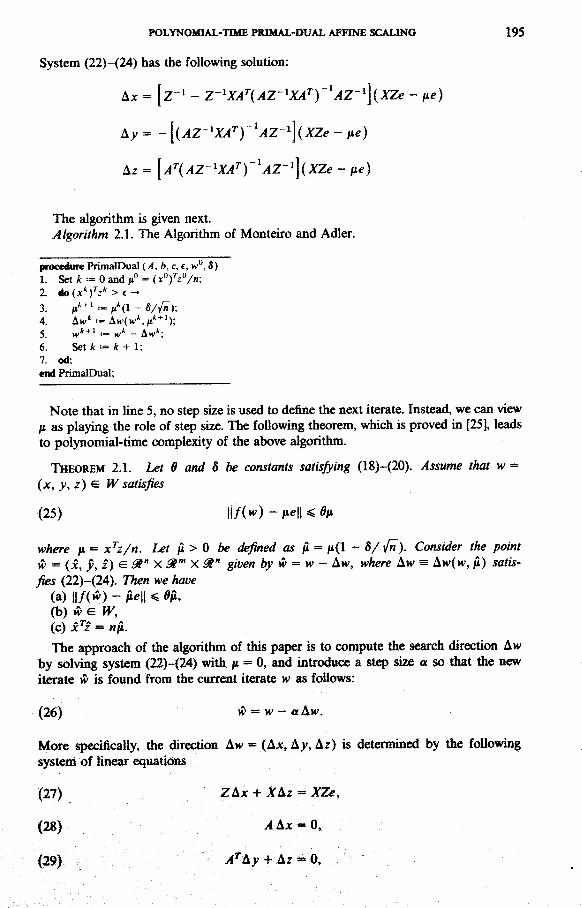
System (22)-(24) has the following solution:

Ax =

Az =

The algorithm is given next.Algorithm 2.1. The Algorithm of Monteiro and Adler.

procedure PrimalDual (/(, b, c, c, w", £)1. Set /t == 0 and /ti" = (x°fz°/n\2. do(x')V>t-»

3. p* + 'i=M*a-S/v'^);4. Aw* ~ AH'(K>*,ft**');5. «,* + '== w*-Aw*;6. Set A: == * + 1;7. od;end PiimalDual;

Note that in line 5, no step size is used to define the next iterate. Instead, we can view/i as playing the role of step size. The following theorem, which is proved in [25], leadsto polynomial-time complexity of the above algorithm.

THEOREM 2.1. Let 8 and 8 be constants satisfying (18)-(20). Assume that w =ix, y, z) e W satisfies

(25) Il/Cw) - Mell < 0,1

where ju = x^z/n. Let ii> 0 be defined as /i = /i(l - 5/\/w). Consider the pointw = (x, y, z) e ^ " X ^ ^ X ^ " given by w = w - Aw, where Aw = Awiw, ji) satis-fies (22)-(24). Then we have

(a) ||/(»^) »i( ) ,(c) x^z = np.The approach of the algorithm of this paper is to compute the search direction Aw

by solving system (22)-(24) with ^ = 0, and introduce a step size a so that the newiterate w is found from the current iterate w as foUows:

(26) w = w - a A w .

More specifically, the direction Aw = (Ax, Ay, Az) is determined by the followingsystem of linear equations

(27) ZAx -I- XAz = XZe,

(28) .4Ax = 0,

(29) ^

1 % RBNATO D. C. MONTEIRO, ILAN ADLER & MAURICIO G. C. REffiNDE

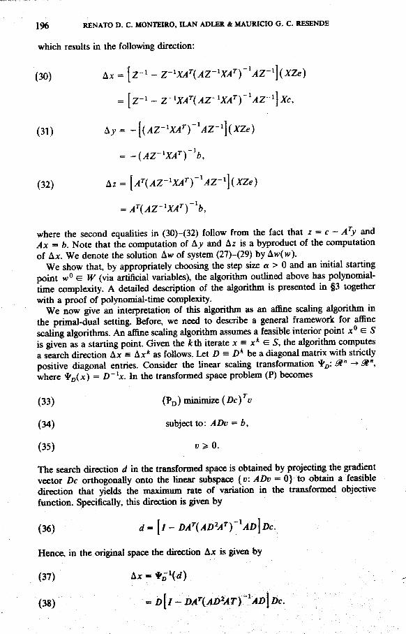
which results in the following direction:

(30) Ax =

(31)

(32) Az = [A'iAZ-'XA'')''AZ-'\iXZe)

where the second equalities in (30)-(32) follow from the fact that z = c - v4'> andAx — b. Note that the computation of A/ and Az is a byproduct of the computationof Ax. We denote the solution Aw of system (27)-(29) by Aw(w).

We show that, by appropriately choosing the step size a > 0 and an initial startingpoint w° eW (via artificial variables), the algorithm outlined above has polynomial-time complexity. A detailed description of the algorithm is presented in §3 togetherwith a proof of polynomial-time complexity.

We now give an interpretation of this algcnithm as an aflBne scaling algorithm inthe primal-dual setting. Before, we need to describe a general framework for affinescaling algorithms. An affine scaling algorithm assumes a feasible interior point x° e Sis given as a starting point. Given the itth iterate x = x* e S, the algorithm computesa search direction Ax s Ax* as follows. Let I> = i)* be a diagonal matrix with strictlypositive diagonal entries. Consider the linear scaling transformation ô: ^" -^ ^",where 'l'o(^) = D~h. In the transformed space problem (P) becomes

(33) (PD) minimize

(34) subject to: ADv = b,

(35) v>0.

The search direction d in the transform«J space is obtained by projecting the gradientvector Dc orthogonally onto the linear subspacs (o: ADv = 0} to obtain a frasibledirection that yields the n^ximum rate of variation in the transformed objectivefunction. Specifically, this direction is given by

(36) d

Hence, in the ori^nal spat* the direction Ax is givrai by

(37) Ax -

(38) ^


Since (P) is posed in minimization form the next iterate Jc s x*" ' is ven by

(39) x = x - a A x ,

where a > 0 is selected so as to guarantee that the iterate x > 0.When the scaling matrix D = X, (38) is the direction generated by the primal affine

scaling algorithm [5], [10], [33]. Note that in this case, the primal aJfine transformation^x maps the current iterate x in the original space into the vector of all ones in thetransformed space. Commonly, for the primal affine scaling algorithm, the step size ais computed by performing a ratio test and multiplying the step size resulting from theratio test by a fixed positive constant less than 1 (see for example [5], [10], [30] and [33]for details).

The primal-dual algorithm can also be viewed as a special case of this generalframework if we assume that besides the current primal iterate x e S, we also have acurrent dual iterate (>?, z) G 7 in the background. In this case, if we let the scalingmatrix D s iZ'^Xf^^, then (38) is exactly the direction given by (30). Note that nowthe current iterate x in the original space is mapped, under the affine transformation*o. into the following vector in the transformed space

(40)

The above framework was described for problems posed in standard form. A similardescription can be done for problems posed in format of the dual problem (D). In thiscase, the affine transformation ^^ is used to scale the slack vector z. When the scalingmatrix D = Z'^, we obtain the dual affine algorithm [1]. More specifically, if (^, z) G Tis the current iterate, the direction computed by the dual affine scaling algorithm isgiven by

(41) Ay= - '

(42) Az = A'

where D = Z'^ and the next iterate iy, z) e T is found by setting y = y - aAy andz = z — a Az. The step size a is computed in a way similar to the one in the primalaffine scaling algorithm and guarantees that f > 0. The dual affine scaling algorithmhas been shown to perform well in practice [1], [2], [20], [23]. In tim dual framework, ifthe scaling matrix D = iZ'^Xf^, then (41) and (42) are identical to (31) and (32)respectively. Thus, in this case, we again obtain the primal-dual affine scaling algo-rithm.

Global, though not polynomial, conveiênce proofs exist for the affine scalingalgorithms under the assumption of nondênera^f [5], [10], [33]. It is conjectured,however, that both the primal and dual affiiw algorithms have worst case tin^complexity that are not polynomial. By appropriately choosing a starting pdmal-dualscûtion and a suitable fixed step size, we show in diis papa- that in the primal-dualsetting, the affine scaling algoritlm }aa& poIynoaual-tiaM con^lexity.

3. H e algo^tan ffinl eomî^sKef^Btt. la tias action, we cd^rfete the <kscnp-tion of the primal-dual affine scaUng algorithm that was briefly outlined in §2Polya(»iiial-tinM OHoplad^ im this a^Hit te is e s t ^ I i ^ ^ by s^ctii^ a i

and 2s& ^{ntqtriate slq} ma. We make <»» fo^ta* as»mipti(»

198 RENATO D. C. MONTEIRO, ILAN ADLER & lAAURICIO G. C. RESENDE

Assumption 3.1. An initial point w° = (x**, y°, z°) G H is given such that thefollowing condition holds:

(43) x°zf = i^°, i = l,2,...,n,

where 0 < M° = 2«< '.Relation (43) is equivalent to requiring that w° = wiii°) where win) is the central

path. Observe that Assumption 3.1 implies (a) and (b) of Assumption 2.1. Given alinear program in standard form, an associated augmented linear program in standardform can be constructed satisfying Assumptions 2.1 and 3.1 and whose solution yieldsa solution for the original problem, if such exists. Indeed, in [25], it is shown that theaugmented problem can be constructed in such a way that a initial point w° lying inthe central path is readily available and that the size of the original problem and thatof the augmented problem are of the same order. The point w° is used as thealgorithm's initial iterate.

The algorithm generates a sequence of points w* e JF, (A: = 1,2,...) starting fromw° as follows. Given w* G W, the search direction AH-CW*) is computed according to(30)-(32) and w*+Ms found by setting

(44) w*"" = w*-a*Aw(M'*)

where a* is the step size at the itth iteration. For the purpose of this paper, which islimited to a theoretical analysis, we choose a constant stq) size a'' = a (for k =0,1,2,...), to be described next. Let c be a ^ven tolerance for the duality gap, i.e. thealgorithm terminates when the duality gap (x*)'z* is no longer greater than e. The stepsize is chosen to depend on the parameter )i°, the dimension n and the tolerance € asfollows:

(45)

where [x] denotes the smallest integer greater than or equal to x. We also assume thata < 1/2, which can be insured by the choice of the tolerance t. Note that the larger«"\ ju° and n are, the smaller the step size a is. We are now ready to describe thealgorithm, which is presented below.

Algorithm 3.1. The Primal-Dual Affine Scaling Algorithm.

pmeeiuK PrimalDualAHIne (.4, j>, c, c, w")1. Set k =- 0;

3. Compute Aw( w*) according to (3OH32);4. Setw**' =-w* - a Aw(w*) where n is a constant given by (45);5. Set * =- A + 1;6. od;e ^ PriiBalDusOAfflne;

A^rithm 3.1 is pven as input the data A, b, c, a tj^ânce £ > 0 for the duality gapstopping criterion and the initial iâte w° as the <Hie qsedfied in Assumption 3.1.

The following theorem, vrtiose proof we defer to later in this section, describes thebduvior <rf ^ e iteraticm of Algorithm 3.1 givm that a gfaxral s t ^ size a is taken.

'Tm.o»Bu3.2. Let w^ ix, y, z) ^ W be given such that

(46) |l/(w) - |i«|f« s max |x,2, - Ml <


where n = x^z/n > 0 and 0 ^ 6 < 1. Consider the point w = ( i , y, z) defined asw = w — a Aw, where Aw = Aw(w) and a G (0,1). Let /i = (1 — a)jtt and

(47)2(1 - «) •

Then we have:(a) ||/(w) - M^(b) Ife<l then(c) ja = x'^z/n.

Theorem 3.2 parallels Theorem 2.1 closely. In spite of the fact that Theorem 3.2 wasformulated in terms of the oo-term, as compared to the 2-nonn formulation ofTheorem 2.1, we should point out that Theorem 3.2 also holds for the 2-nonn as willbecome clear from its proof. The reason we state Theorem 3.2 in terms of the oo-normis discussed in the next section where we prove convergence (not necessarily pol5mo-mial) of algorithm 3.1 for any given starting point w" G W. Polynomial convergencewill only be guaranteed in the case that the initial starting point is in some sense closeto the central path. In that context, the oo-norm wiU play an important role.

We can view / (w) as a map from ^ " X '" X Si" into 01", mapping w = (x, y, z)into the complementarity vector XZe. Under this map, the set W is mapped onto thepositive orthant, the central path T is mapped onto the diagonal line / ( F ) = {jue;JU > 0} and an optimal solution w* = (x*, y*, z*) for the pair of problems (P) and (D)is mapped into the zero vector [25]. The image under / of the set of points w G ^F suchthat | | / (w) — fi,e\\ < tf/x with /i = x^z/n is a cone in the positive orthant of Si" havingthe diagonal line / ( F ) as a central axis and the zero vector as an extreme point. Thecentral axis forms a common angle with all the extreme rays of the cone and this angleis an increasing function of 0. For this reason, we refer to ^ as the opening of the cone.Theorem 2.1 states that if we start at a point inside this cone, then all iterates willremain within the same cone and will approach the optimal solution /(w*) at a rategiven by (1 — 8/ v^). ITiis is to be contrasted with Theorem 3.2, where the iterates areguarante^ to be in cones with openings that âdually increase from one iteration tothe other.

Note that by (c) of Theorem 3.2, we have

(48) x ^ F = «/I = (1 - a)ny. = (1 - a)x^z

that is, the duality gap is reduced by a factor of (1 - a) at each iteration. Therefore, itis desirable to choose a as large as possible in order to obtain as large as possible adecrease in the duality g ^ . Once a is specified, the number of iterations necessary toreduce the duality gap to a value < e is not grîter than

(49) Kâ

which is immediately implied by IIK fact that

(50) (x'^)V=(l-«)''(x°)V=(l-«)%»<£

wh«e flie second equality is due to (43) and the iiuquality fdlows by the choi(» of K.Th& dmix ot a should now be m ^ to piaiantM feasibility of all ita-ates w*,{* = 0 , 1 , . . . , AT) and ti^vard tfiis obgectiw, (b) <rf Tbeatxm 3.2 wiU play an important

200 RENATO D. C. MONTEIRO, ILAN A0LER & MAURICIO G. C. RESENDE

role. The choice of a given by relation (45) becomes clear in the proof of the followingresult.

COROLLARY 3.3. Let K be as in (49) and consider the first K iterates generated byAlgorithm 3.1, i.e. the sequence { w*}f_o- ^ ' M* = (1 " « ) V o"^ ^* = *««^ M allk = 0,1,2,..., K. Then, for all k = 0,1,2,..., K we have:

(a) Wfiw") - Mo. < O'li",(b) w* G JF,(c) ix'')V/n = /I*.

PROOF. From (45), (49) and the definition of 0'', it follows that

(51) fi* < Kna^ = 1

for all fe = 0 ,1 , . . . , K. The proof of (a), (b) and (c) is by induction on k. Obviously(a), (b) and (c) hold for fe = 0, due to Assumption 3.1. Assume (a), (b) and (c) hold forfe, where 0 < fe < AT. Since a < 1/2, it follows that

In view of the last relation, we can apply Theorem 3.2 with w = w'', /* = M*9 = 0'' io conclude that (a), (b) and (c) hold for fe + 1. This completes the proof of thecorollary. •

We now discuss some consequences of the above corollary. Let L denote the size oflinear programming problem (P). If we set e = 2~°<^', then by (50), the iterate '^generated by Algorithm 3.1, where K is given by (49), satisfies ix'^)V < e = 2°Then, from w*^, one can find exact solutions of problems (P) and (D) by solving asystem of linear equations which involves at most O(/i^) arithmetic operations [27J.Using this observation, we obtain the main result of this section.

THEOREM 3.4. Algorithm 3.1 solves the pair of problems iP) and iD) in at mostiterations, where each iteration involves Oin^) arithmetic operations.

PROOF. From (45), (50) and the fact that e = 2-<'('> and jn-= 2 < >, it follows thatthe algorithm takes at most

(53) K=

iterations to find a point w'' e W satisfjmg (;c*)^z* < e = 2~^^\ TTie woric in eachiteration is dominated by the effort required to compute and invert the matrix

( )" ' .Y*/ i^ , namely, O(n') arithmetic operations. This proves the theorem. •We now tum out attention towards proving Theorem 3.2. ITie proof requires some

technical lemmas.

LEMMA 3.5. Letw = ix, y, z) e W be given. Consider the point w = ( i , y, z) givenby w = w - a Aw, where Aw = AW(H') = (AJC, Ay,Az) and o > 0. Then we have:

(54) x,Zi = (1 - a)XiZ, + aÂxiAzt and

(55) y^


PROOF. First, we show (54). We have:

= x,.z, - a(x,.A2, + 2,.A.x,.) -I- ^ ,

= XfZi - aXjZ^ + aÂx, Az,

= (1 - a)XiZi + aÂjt, Az,

where the third equality is implied by (27). This completes the proof of (54). To show(55) multiply (28) and (29) on the left by (Aj)^ and (Ax)^, respectively, and combinethe two resulting expressions. This shows (55) and completes the proof of the lemma.

•The next lemma appears as Lemma 4.7 in [25], where it is proved.

LEMMA 3.6. Let r, s and t be real n-vectors satisfying r -¥ s — t and r^s > 0. Then wehave:

(56) max(|lr||,l|5|l)<||/||,

(57) \\RSe\\ < Jlf^

where R and S denote the diagonal matrices corresponding to the vectors r and s,respectively.

As a consequence of the previous lemma, we have the following result.

LEMMA 3.7. Let w = (JC, j , z) e W be given. Consider the direction Aw s A»v(w)= (Ax, t^y, Az). Define A / G ^ " as Af = iAXXAZ)e, where (AA') and iAZ) arethe diagonal matrices corresponding to Ax and Az, respectively. Then we have

(58) ^

PROOF. Let D = iZ'^Xf^\ Multiplyit^ both sides of (27) by (XZ)'^/^ we have

(59) D-Â f'^

By (55) we have that (D~Âx)^(Z>Az) = 0. Hence, we can apply Lemma 3.6 withr = D-Âx, s = DAz and / = iXZ)^^h resulting in

(60) ^

which is equivalent to (58). This con4>letes the proof of the lemma. •We are now ready to prove Thewem 3.2.PROOF (THEOREM 3.2). From (54) and the fact that /i = (1 - a)n, it follows that

(61) Jc,z, - M - (1 - a)ixiz, -ii) + aÂx, Az,.


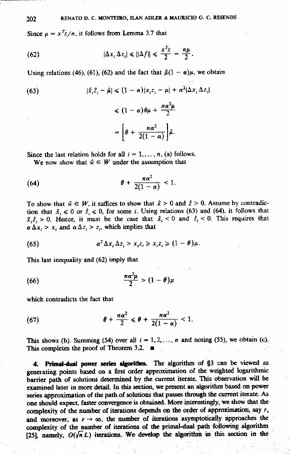
Since fi — x^z/n, it follows from Lemma 3.7 that

(62) | A x , A z , | ^ ^

Using relations (46), (61), (62) and the fact that /i(l - a)/i, we obtain

(63) \xfi, - Al < (1 - «)|Jf,2, - Ml + A^î ' /l

2(1 - a)

Since the last relation holds for aU / = 1,.. . , «, (a) follows.We now show that w ^W under the assumption that

^ ' 2(1 - a)

To show that w e^ W,it suffices to show that Jc > 0 and f > 0. Assume by contradic-tion that jC; < 0 or z, < 0, for some /. Using relations (63) and (64), it follows thatJc,z, > 0. Hence, it must be the case that Jc, < 0 and f, < 0. This requires thato Ax, > X, and aAz, > z , which implies that

(65) aÂx,Az,>x,Z;>x,z,

This last inequality and (62) imply that

(66) ^ > (1 -

which contradicts the fact that

(67) e 2(1 - a)

TTiis shows (b). Summing (54) owr all i = 1,2,..., n and noting (55), we obtain (c).This completes the proof of Theorem 3.2. •

4. Prinud-dini power serfes dgmittm. Tlie algorithm of §3 can be viewed asgenerating points bas^ on a first order approximation of the weighted logarithmicbarrier path of solutions detarmined by the current iterate. This obsCTvation will beexamined later in more detail. In tins section, we present an al^mthm b a ^ on powerseri» approximation of the path of solutions tiiat pass^ thro i^ the current ito-ate. Asone shcHild expect, faster ocmvergmce is obtained. More interratin^y, we show that fliecomplexity of the numl^^ of itraatirais diepouis on Vbe order of i^proximation, say r,and nK)reover, as r -• oo, the nuiid>» of iteratimis asyn^toticaDy approaclos thecomplexity of tl« numba- of ita^ti(»is of titt primal-dual pafli fcôwii^ algorithm[251 nairoly, O{fiL) iteratiaas. We dea^qp tire a%orithm in this %cti(m in te


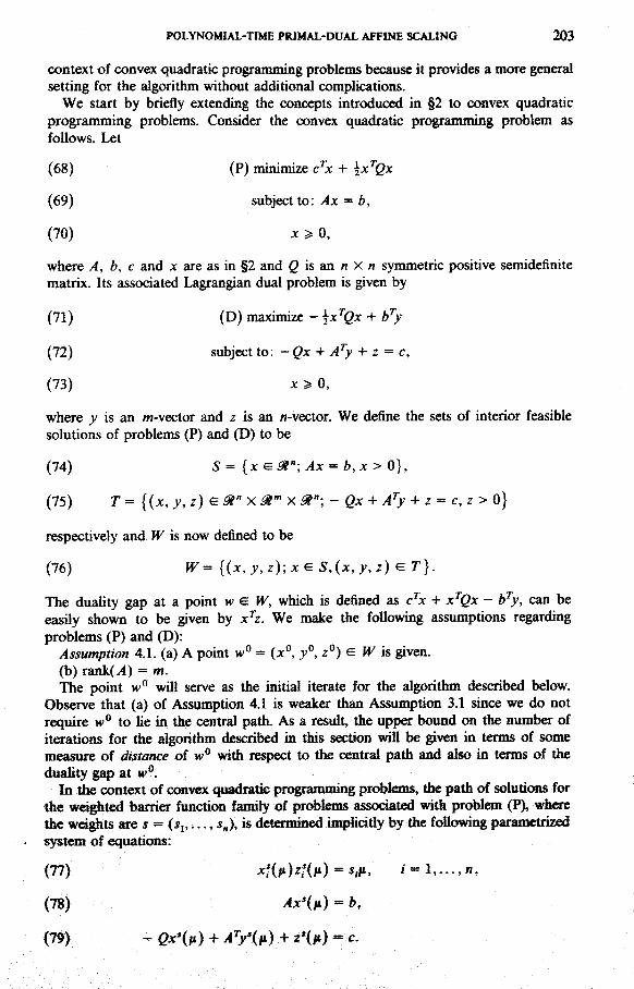
context of convex quadratic programming problems b«:ause it provides a more generalsetting for the algorithm without additional complications.

We start by briefly extending the concepts introduced in §2 to convex quadraticprogramming problems. Consider the convex quadratic programming problem asfollows. Let

(68) (P) minimize c^x -\- ^x^Qx


(70) X > 0,

where A, b, c and x are as in §2 and 2 is an n X w symmetric positive semidefinitematrix. Its associated Lagrangian dual problem is given by

(71) (D) maximize - \x^Qx + b^y

(72) subject to: -Qx + A^y + z = c,

(73) x>0,

where y is an w-vector and z is an «-vector. We define the sets of interior feasiblesolutions of problems (P) and (D) to be

(74) 5 = {xG^"; .4x = fc,x>0},

(75) T = {(x, y, z) G ^ " X ^ ^ X ^" ; - gx -I- /1 >' + z = c, z > 0}

respectively and W is now defined to be

(76) JF= { ( x , > ' , z ) ; x G S , ( x , j , z ) G r } .

The duality gap at a point w G W, which is defined as c x -I- x^Qx - b^y, can beeasily shown to be given by x^z. We make the following assumptions regardingproblems (P) and (D):

Assumption 4.1. (a) A point w° = (x°, j " , z°) G W is given.(b) rank(^) = m.The point w" will serve as the initial iterate for the algorithm described below.

Observe that (a) of Assumption 4.1 is weaker than Assumption 3.1 since we do notrequire w" to lie in the central path. As a result, the upper bound on the number ofiterations for the algOTithm described in this section will be given in terms of somemeasure of distance of w° with r«pect to the central path and also in terms of theduality g ^ at w°.

In the context of convex quadratk; programming protâm, tte path of solutions forthe wdghted barrier function family of pr<Alems assodated with problem (P), whwethe wd^ts are s = (JJ, . . . , sJ, is detamined inqjlidtly by the following paiait»tTizedsyston of equations:

(77)

(78) Ax'ifi) - b,

<79) - Qx'iii) -h ^ V(#) + z'ifi) = c.


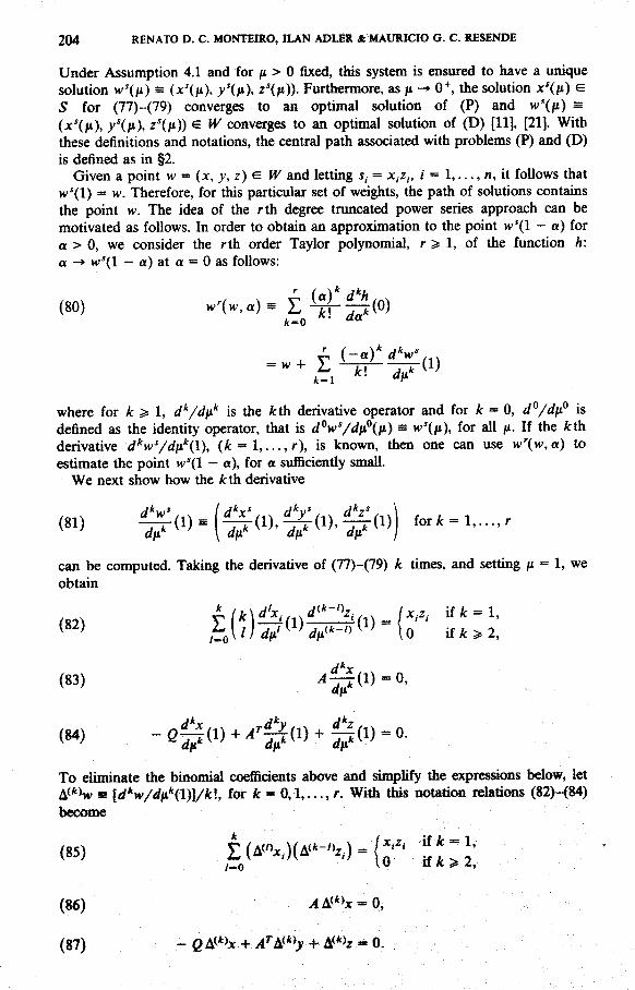
Under Assumption 4.1 and for ja > 0 fixed, this system is ensured to have a uniquesolution w'in) = {x'(fi), y'(ii), z'ifi,)). Furthermore, as ju -• 0" , the solution x'(p.) eS for (77)-(79) converges to an optimal solution of (P) and w'ifi) =ix'in), y'iii), z'iii)) e W converges to an optimal solution of (D) {11], [21]. Withthese definitions and notations, the central path associated with problems (P) and (D)is defined as in §2.

Given a point w = (x, y, z) e. W and letting s, = x,z,, j = 1,. . . , n, it follows thatw'(l) = w. Therefore, for this particular set of weights, the path of solutions containsthe point w. The idea of the rth degree truncated power series approach can bemotivated as follows. In order to obtain an approximation to the point ^ ' ( l - a) fora > 0, we consider the rth order Taylor polynomial, r > 1, of the function h:a -» w%l - o) at a = 0 as follows:

(80) w'iw,a)= Z •k-O

where for k ^ 1, d''/d[i'' is the kih derivative operator and for k = 0, d'^/dix° isdefined as the identity operator, that is d%'/dii°iii) = w'in), for all /i. If the kthderivative d''wydn''il), ik = l,...,r), is known, then one can use w''iw,a) toestimate the point w'(l - a), for a sufficiently small.

We next show how the A:th derivative

can be computed. Taking the derivative of (77)-(79) k times, and setting /a = 1, weobtain

(83) ^0(1) - 0,

(84, _ 2 0 ( 1 ) * ^ '0(1) + 0 (1 ) -0 .

To eliminate the binomial coefficients above and simplify the expressions below, letA<*>w s [d''w/dn''(l)]/kl, fot k = O,l,...,r. WiA this notation rdations (82)-(84)become

Ly\)(^-".)-{r 'All:(86)

(87) - eA<*>jc + '"A<*>j-1-A<*>z - 0.

POLYNOMUL-TIMB PRIMAL-DUAL AFFINE SCAUNG 205

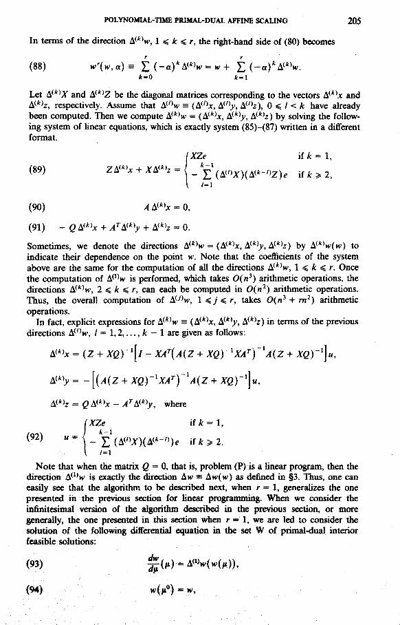
In terms of the direction A<*>w, 1 < it < r, the right-hand side of (80) becomes

(88) w'iw,a)= £(-a)*A<*>w = w+ f (-a)*A<*Vk~0 k~l

Let A *'A' and A'**Z be the diagonal matrices corresponding to the vectors A<*'x andA<*'z, respectively. Assume that A ' w = (A<' x, A^'^, A<"z), 0 ^ I < k have alreadybeen computed. Then we compute A**w = (A<*'x, A<*'>', A**'z) by solving the follow-ing system of linear equations, which is exactly system (85)-(87) written in a differentformat.

XZe(89)

(90) A A'*>x = 0,

(91) - Q A<*'x + vl A<*>>' + A<*'z = 0.

Sometimes, we denote the directions A*>w = (A<*>x, A^ 'j-, A<*>z) by A<**w(w) toindicate their dependence on the point w. Note that the coefficients of the systemabove are the same for the computation of all the directions A *'w, 1 < *: < r. Oncethe computation of A^^^w is performed, which takes O(n^) arithmetic operations, thedirections A<*>w, 2 < it < r, can each be computed in Oin^) arithmetic operations.Thus, the overall computation of A ^ w, 1 < 7 < r , takes O(w^ + TTJ ) arithmeticoperations.

In fact, exphcit expressions for A<*'w = (A ' 'x, A^''^y, A<*>z) in terms of the previousdirections A^'^w, I = 1,2,..., k — 1 ate given as follows:

= (Z

A<*>z = Q A<*>x - /4 A<*V, where

(XZe itk = l,

(92) u = ' '-' ( ) ( - ' ) ) e itk>2./-I

Note that when the matrix Q = Q, that is, problem (P) is a linear prcâm, then thedirection A 'w is exactly the direction Aw s Aw(w) as defined in §3. Hius, one caneasily see that the algorithm to be described next, when r = 1, generalizes the onepresented in the previous section for linear prcâmming. When we consider theinfinitîmai version of the algorithm de»:ribed in the previous section, or moregenerally, the one presented in this s«:tion «1ien r = 1, we are led to consider thesolution of the following differoatiid equation in the set W of primal-dual interiorfeasible sduticms:

(93) ^ ( M )

(94) w ( / ) = w.


where /t° and w = (x, y, z) e W axe assumed given and (94) determines the initialcondition for (93). The trajectories of the diflferential equation (93) are said to beinduced by the vector field w e Jf -» A<^)(H') e ^ " X ^"^ X ^" . It turns out, by theway we motivate our algorithm, that the trajectory induced by this vector field andpassing through the point w = (x, y, z) is exactly the locus of points traced by thepath of solutions w'in) of system (77)-(79) when the wdghts s = (sj, ...,*„) are givenby J, = XfZi.

Before w e descr ibe the a lgor i thm based o n the r t h degree t runca ted power senes , weneed t o in t roduce some further no ta t ion . F o r w e W, let f ^ ) i y ; ( )a n d fr^s u m p t i o n 4.1 a n d let

(95)

duce some furthe , f^) i^,^,y;(= max,^,^„/((>!'). Consider now the point w° e W mentioned in As-

Note that 6° < 1 and that /i° and 8° satisfy

(97) lt/(w°)-All«<«V-

The fact that we are using the oo-norm is crucial here in order to guarantee that, givenw° G W, there exist constants /i° and 6° such that tf° < 1 and such that relation (97)holds. In general, given any w^ e W, the above property does not hold if we use the2-norm. This is the main reason for using the oo-norm instead of the 2-nonn.

We now have all the ingredients to describe the truncated power series algorithm ofdegree r. The truncated power series algorithm of degree r studied in this sectiongenerates a sequence of points w''G W (k = 1,2,...), starting from the point w° e W(cf. Assumption 4.1) as follows. Given w* e W, w*"- is found by setting w^^^ =H-XH-*, a) (cf. (88)), where a > 0 is the step size. As in §3, we assume that the samestep size is used for all iterations. TTie step size a > 0 is determined as follows. Let£ > 0 be a tolerance for the duality gap (x*)^(z*), so that, like in §3, we terminate thealgorithm as soon as (x*)^(z*) < «. The step size is detennined as a function of thedegree of approximation r, the dimension «, the parameter /i°, the constant ff° andthe tolerance c as follows:

(98)

where y = 2/(1 - 0°) and q(r) =sively as follows:

(99) pil) = 1,

with the sequence pik) defined recur-

t(100) p(fc)= tpij)pik-j), k>2.

We also assunse that the tolerance c is given small enou^ to ensure that o < 1/2. TTiesolution of the recurrence relation (99)-(100) is well known and is given by

The following estimate of ^ wll be useful later.

POLYNOMIAL-TUKIE PRIMAL-DUAL AFFINE « ;AUNO 207

LEMMA 4.2. sup^qir)^^'' < 16.

PROOF. Using the formula for pik) above and the fact that (2) < 2" for all n andyt < «, we obtain

(102) qir)^ E

and this completes the proof of the lemma. •We are now ready to describe the algorithm, which is presented below.Algorithm 4.1. The Truncated Power Series Algorithm of Degree r.

procedive TruncatedPowerSeries (a, fr, c, t, tf")1, Set k ••= 0;2, do(;c*)^2* > £ - >3, Compute A'*'H'(K'*), for fe = 1,2,,,,, r, as described above;4. Set w**' != iv'(iv*, a) where o is the constant given by (98);5. Setk~k + 1;6. ad;end TruncatedPowerSeries;

The next theorem is a generalization of Theorem 3.2.

THEOREM 4.3. Let w = ix, y, z) e^ W and ^> 0 be given such that

(103) II/(H') - M L = max

for some 0 ^B <l. Consider the point w = (x, y, z) given by w = w\w, a), wherea e (0,1). Let ji.^ il - a)(i and

(104)

Then we have:(a) | | / (w) - / l L /(b) / / e < 1 then w G W.

Note that the opening of the cone described in tiie discussion following Theorem 3.2gradually increases by a term that depends on the fc-powers of the step size, r -f- 1 < A:< 2r. The consequences of Theorem 4.3 are as follows.

COROLLARY 4.4. Let K^^ a~^nn(2we~ V°)l- Consider the first K iterates generatedby Algorithm 4.1, that is, the sequence {w''}^^^. Let /i* = (1 - a ) V

(105) 9''= 9"

Then, for all k = 0,1,..., K, we have(a) Wfiw") - M* |U < «V-(b)^*^!^.(c) <x*)^(z * * *

208 RENATO D. C. MONTIEIRO, ILAN ADLER & MAURICIO G. C. RESENDE

PROOF. From the definition of d*, K, relation (98) and the fact that y =2/(1 - 6% we have that for all A: = 1,2,..., A"

(106) <?*<<?"

Since e° < 1, it follows that tf * < 1 for A: = 1,2,..., ,^. Note that (a) and the fact thattf * < 1 immediately imply (c). The proof of (a) and (b) is by induction on k. Obviously(a) and (b) hold for A = 0 due to (97) and Assumption 4.1. Assume (a) and (b) hold fork, where 0 ^ k < K.We will show that (a) and (b) hold for A: + 1. If

(107)

then, by applying Theorem 4.3 with w = w*, H' = W*^S /* = M* ^^d tf = tf *, it followsthat (a) holds for A: + 1 and that (b) also holds for i + 1 since tf*^* < 1. Therefore,we only have to show (107) to complete the proof of the corollary. Note that (106)implies that

(108) 1 - tf* > ^ - ^ = y - i .

Using relation (98), (108) and the fact that (1 -h tf*) < 2, one can easily verify that

Hence, from the definition of qir), tf* and the fact that a < 1/2, it foUows that

tf* +

tf*

POLYNOMLAL-TIME PRIMAL-DUAL AFFINE SCALING 209

where in the third inequality we use the fact that (1 + »*) < 2 and (1 - ^* ) " ' < y.This shows (107) and concludes the proof of the corollary. •

As an immediate consequence of the above theorem, we have the following result.

COROLLARY 4.5. The total number of iterations performed by Algorithm 4.1 is on theorder o/0(<pn('*i>/^[max(log«,log£-Mog/i°)]<'^'/''), where q> ^ f^^(w'')/f^îw%

PROOF. Let

(110) ^ = a

By (c) of Corollary 4.4, it follows that

(111) (x'^)^z*^

where the last inequality follows from the definition of K. Hence, Algorithm 4.1performs no more than K iterations. Using (96) and the fact that y = 2/(1 - ^°), itfollows that

(112) Y < 2/^(w<')//^^(w°).

By using the last relation, expressions (110), (98) and Lemma 4.2, the corollary follows.•

Let L denote the size of the convex quadratic programming problem (P). Then if weset € = 2~''^^\ then the observation preceding Theorem 3.4 still holds in the context ofconvex quadratic programming problems. Using this observation, we can now state themain result of this section, which is a direct consequence of the previous corollary.

THEOREM 4.6. / / the initial iterate is such that f^w^) = 2'^^'> and the ratio

(113) /™ax(>^°)//min(H'°) = 0( l )

then Algorithm 4.1 solves the pair of problems (P) and (D) in at most

(114) O(/i^<iî/"L<i^'/'>)

iterations, where each iteration involves Oin^ + n^r) arithmetic operations.

We now tum our effort towards proving Theorem 4.3. The next result generalizesLemma 3.5.

LEMMA 4.7. Let w = ix, y, z) e W and a>0 ge given. Consider the point w =

( x , y, z) defined as w ^ w'iw, a). Then we have:

(115) x,f, = (1 - a)x,z, + E ( - l ) V i (A<%,)(A<'-»z,),l-r+l J-t-r

(116) iA^^h^


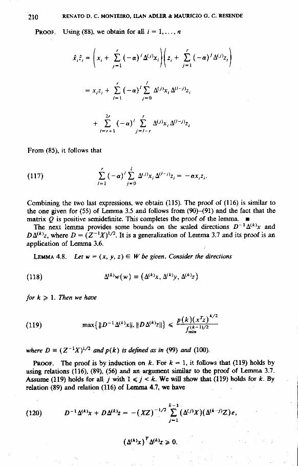
PROOF. Using (88), we obtain for all / = 1 , . . . , n

J-l I\ y-1

r I

l~\ y-0

+ I (-«)' I

From (85), it follows that

(117) t (-«)' E/-I y-O

Combining the two last expressions, we obtain (115). The proof of (116) is similar tothe one given for (55) of Lemma 3.5 and follows from (90)-(91) and the fact that thematrix Q is positive semidefinite. This completes the proof of the lemma. •

The next lemma provides some bounds on the scaled directions i)~Â**'x and£)A'*'z, where D = (Z'^xy^^. It is a generalization of Lenuna 3.7 and its proof is anapplication of Lemma 3.6.

LEMMA 4.8. Let w = (jc, y, z) ^ W be given. Consider the directions

(118) A(*>w(w) = (A<*>x, AWj', A<*>z)

for k ^ 1. Then we have

(119) max{l|i)-iA<*);cl|, ||Z)A(*>z||} < ^^%^! ,^^ '/min

where D s (Z'^Xf^^ and pik) is defined as in (99) and (100).

PROOF. The proof is by inducticm on *:. For A: = 1, it follows that (119) holds byusing relations (116), (89), (56) and an aiûment similar to the proof of Lemma 3.7.Assume (119) holds for all j with 1 < y < k. We will show that (119) holds for fe. Byrelation (89) and relation (116) of Lemma 4.7, we have

(120) i)-»A<*>;c + Z)A<*>z = - ' / '

POLYNOMIAL-TIME PRIMAL-DUAL AFFINE SCAUNG

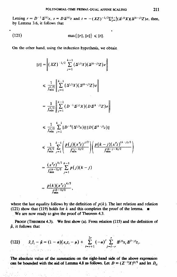
Letting r = Z)-'A<*>;c, s = Z)A<*>2 and t = -by Lemma 3.6, it follows that

211

?, then.

(121)

On the other hand, using the induction hypothesis, we obtain

k-\

(A<>>A')(A<*-»Z)e

1fl/2/mm

k-\

min y = 1

.k/2

where the last equality follows by the definition of pik). The last relation and relation(121) show that (119) holds for k and this completes the proof of the lemma. •

We are now ready to give the proof of Theorem 4.3.

ftioOF (THEOREM 4.3). We firat show (a). From rdation (115) and the definition offi, it follows that

(122)J-l-r

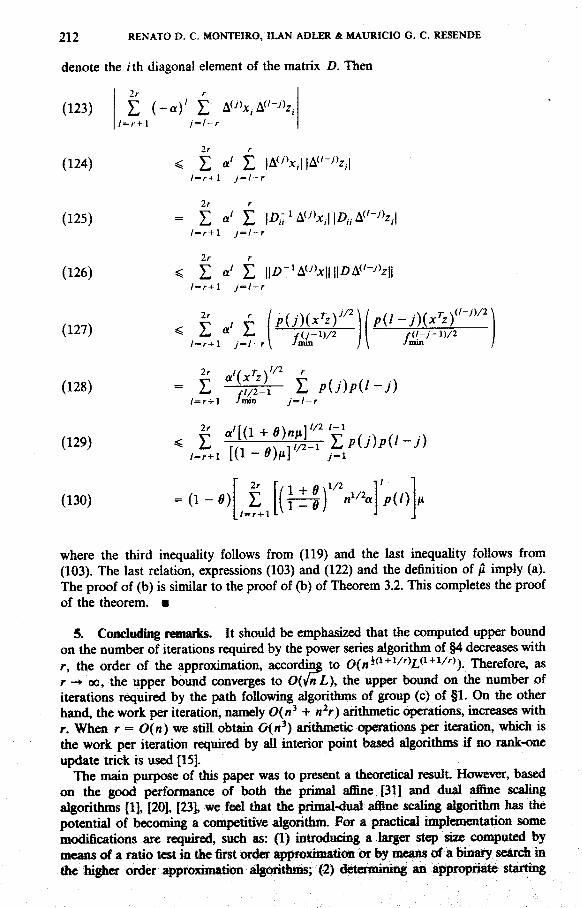
The £A>S(dute vali» of the sumnmlicHi on the li^t-haad s i ^ of the abow expiesacmcaa be bmoulal with ^ aid of Lemma 4.8 as fcdlows. Let D s {Z'^Xf'^ and let Dî


denote the /th diagonal element of the matrix D. Then

Ir

(123)

(124)

(125)

(126)

(-a)'

t cc' i |A<»x,.| |A<'-»z,.|

E «' E IA7'A<»x,.||A,A<'->>z,.|- r + l J = l-r

Z cc' t ||Z)-'A(»x||||/3A<'-»z||

(127)

(128)

(129)

(130)

Jo

ll fl/2-l i-l/—r+l /min

E/-r+l

= (! -<?)

where the third inequality foUows from (119) and the last inequality follows from(103). The last relation, expressions (103) and (122) and the definition of p. imply (a).The proof of (b) is similar to the proof of (b) of Theorem 3.2. This completes the proofof the theorem. •

5. Ctmcluding rranarks. It should be emphasized that the computed upper boundon the number of iterations required by the power series algorithm of §4 decreases withr, the order of the approximation, according to O(H^*^'^^''''^L^^^^^''^). Therefore, asr -» 00, the upper bound converges to OiynL), the upi»r bound on the number ofiterations r«}uired by the path following algorithms of group (c) of §1. On the otherhand, the work per iteration, namely O(n' + nV) arithmetic C5)erations, increases withr. When r = <9(n) we still obtain O(n^) arithmetk op«ations pet iteiation, whidi isthe work per iteration required by all interior point bas^ algcffidims if no rank-oneupdate trick is used [15].

The main purp(»e of this p^per was to prraait a theoretical result. However, basedon the good performance of both the primal affine [31] and dual affine scalinga^rithmis [1], [20], [23], we fed that the primal-dual affine scaling aôrithm has thepotential of becoming a ccMnpetitiw algorithm. For a practical in^laoentation somemodifications are required, such as: (1) introdudng a larger stq) sae conapoted bymeims of a ratio test in the first ordra' ap{»oxiniati<c» or 1^ means of a biaary search intfie high^ order ^jproximation aôrithms; (2) detoB^mig an ajpfpr Hiate

POLYNOMIAL-TIME PRIMAL-DUAL AFFINE SCAUNG 213

artificial problem that gives a good initial starting point; and (3) making a good choiceof r.

Note that when r = 1, the primal-dual affine scaling algorithm described in §3 canbe viewed as a simultaneous application of an affine scaling algorithm to the primaland dual problems, which implies that both the primal and dual objective functionsmonotonically approach the optimal value. For a practical implementation, thissuggests that two ratio tests performed independently in the primal and the dual spacesrespectively, might outperform one ratio test done simultaneously in the primal-dualspace, since a larger decrease in the duality gap would be obtained. On the other hand,the last strategy would be more conservative in the sense that it would keq? the iteratesfrom coming too close to the boundary of the primal-dual feasible region.

References[1] Adler. I., Kannarkar, N., Resende, M, G. C. and Veiga, G. (1989). An Implementation of Karmarkar's

Algorithm for Linear Prcâinming. Math. Programming 44.[2] , , and (1989). Data Structures and Programming Techniques for the

Implementation of Karmarkar's Algorithm. ORSA Journal on Computing 1 84-106.[3] Anstreicher, K. M. (1986). A Monotonic Projective Algorithm for Fractional Linear Programming.

Algorilhmica 1 483-498.[4] (1989). A Combined 'Phase I-Phase IF Projective Algorithm for Linear Programming. Math.

Programming 43 209-223.[5] Barnes, E. R. (1986). A Variation on Karmarkar's Algorithm for Solving Linear Programming

Problems. Math. Programming 36 174-182,[6] Bayer, D. and Lagarias, J, C. (1989). The Nonlinear Geometry of Linear Programming. I. Affine and

Projective Scaling Trajectories. Trans. Amer. Math. Soc. 314 499-526,[7] and (1989). The Nonlinear Geometry of Linear Programming, IL Legendre Transform

Coordinates and Central Trajectories. Tram. Amer. Math. Soc. 314 527-581.[8] de Ghellinck. G. and Vial, J.-F, (1986). A Polynomial Newton Method for Linear Programming.

Algorithmica I 425-454.[9] DSun, \. I. (1%7). Iterative Solution of Problems of Linear and Quadratic Programming. Soviet Math.

Dokl. 8 674-675.(10] (1974). On the Speed of an Iterative Process, Upravlyaemye Sistemi 12 54-60. In Russian,[11] Fiacco, A, V, and McCormick, G, P, (1%8). Nonlinear Programming: Sequential Unconstrained

Minimization Techniques. John Wiley and Sons, New York.[12] Frisch. K, R. (1955). The Logarithmic Potential Method of Convex Programming. Technical report.

University Institute of Economics, Oslo, Norway.[13] Gonzaga, C. C, (1989), An Algorithm for Solving Linear Programming in O(n^L) Operations, In

Nimrod Megiddo. editor. Progress in mathematical programming-Interior-point and related methods.Springer-Verlag, 1-28.

[14] (1989). An Conical Projection AlgoriUun for Linear IVogramming, Math. Programming 43151-173.

[15] Karmarkar, N, (1984). A New Polynomial-Time Algorithm for Linear Programming. Combinatorica 4373-395.

[16] (1984). Talk given at the University of California, BeAeley.[17] and Lsârias, J.. Slutsman, L., and Wang, P, (1989), Power Series Variants of Karmarkar-type

Algorithms. AT&T TechnicalJoarmU 68(3) 20-36,[18] Ktîma, M,, Mizuno, S, and Yoshise, A, (1989), A Polynomial-Time Algorithm for a Qass of Linear

Ccnnplementarity Prc*lems, Mathematical Programming 44 1-26,[19J , and (1989), A Primal-Dual Interior Point j ô r i thm for Linear Program-

ming, In Nimrod Megiddo, editor. Progress in mathematical programming-Interior-point and relatedmethods. Springer-Veriag, 29-48,

[20] Marsten, R, (1987). The IMP System on Personal Cwaûters, Presentation given at the ORSA/TTMSJoint National Meeting. S t Louis, MO.

[21] Meîddo, N, (1989), Pathways to the C^tiraal Set in Utieai PKâamung, In Nimrod M ^ d d o , «litor,Propess in mathematical prop'omming-lnterior-point and related methods. Springer-Veriag, 131-158,

[22] and Shub. M, (1989), Boumiary Bdavioiir of Interior Point A l ^ t h m s in Liiwar Program-ming, Mathematics cfOpavtioas Raearch 14 97-146,

[23] Monma, C, L, aiKl M<»n<», A. J, (1M7). Ctmpatiôtai Experimental tirith a Dual Affine Variant ofKarmarkar's MeAod bx L U K K Ifti^ranmiing, Operatima Res^rch Letters 6 261-267.


[24] Monteiro, R, D. C, and Adler, I. (1987). An Extension of Karmaritar Type Algorithm to a Qass ofConvex Separable Programming Problems with Global Linear Rate of Convergence. TechnicalReport ESRC 87-4, Engineering Systems Research Center, Univ«sity of Califonria, Berkeley, CA94720, 1987, To s^pear in Mathematics of Operations Research.

[25] and (1989), Interior Path Following Primal-Dual Algorithms—Part I, Linear Pro-gramming, Math. Programming 44 27-42,

[26] and (1989). Interior Path Following Primal-Dual Algorithms—Part II: ConvexQuadratic Programming. Math. Programming 44 43-66,

[27] Papadimitriou, C. R, and SteigUtz, K, (1982). Combinatorial Optimization: Algorithms and Complexity.Prentice-Hall, Englewood Cliffs, NJ.

[28] Renegar, J, (1986), A Polômial-Time Algorithm Based on Newton's Method for Linear Program-ming, Technical report MSRI07 118-86, Mathematical Sciences Research Institute, Berkeley, CA, Toappear in Math. Programming 40.

[29] Todd, M. J, and Burrell, B, P. (1986), An Extension to Karmarkar's Algorithm for Linear Program-ming Using Dual Variables, Algorithmica I 409-424.

[30] Tomlin, J, A. (1985), An Experimental Approach to Karmarkar's Projective Method for LinearProgramming. Technical report, Ketron, Inc., Mountain View, CA.

[31] and Welch, J, S. (1986), Implementing an Interior Point Method in a Mathematical Program-ming System, Technical report, Ketron, Inc., Mountain View, CA.

[32] Vaidya, P, M. (1987). An Algorithm for Linear Programming Which Requires O{{(m + n)n^ + (m +« ) " ) / . ) Arithmetic Operations. Technical report, AT&T Bell Laboratories, Murray Hill, NJ, 1987.To appear in Mathematical Programming.

[33] Vanderbei, R. J,, Meketon, M, S. and Freedman, B. A. (1986), A Modification of Karmarkar's LinearProgramming Algorithm, Algorithmica 1 395-407,

[34] Ye, Y. and Kojima, M, (1987). Recovering Optimal Dual Solutions in Karmark's PolynomialAlgorithm for Linear Programming. Math. Programming 39 305-317,

MONTEIRO- A T & T BELL LABORATORIES, HOLMDEL, NEW JERSEY 07733,ADLER: DEPARTMENT OF INDUSTRIAL ENGINEERING AND OPERATIONS RESEARCH,

UNIVERSITY OF CALIFORNL\, BERKELEY, CALIFORNL\ 94720

RESENDE: A T & T BELL LABORATORIES, MURRAY HILL, NEW JERSEY 07974