Full Terms & Conditions of access and use can be found athttp://www.tandfonline.com/action/journalInformation?journalCode=tgnh20
Download by: [203.128.244.130] Date: 15 March 2016, At: 00:40
Geomatics, Natural Hazards and Risk
ISSN: 1947-5705 (Print) 1947-5713 (Online) Journal homepage: http://www.tandfonline.com/loi/tgnh20
A stochastic model for earthquake slip distributionof large events
S.T.G. Raghukanth & S. Sangeetha
To cite this article: S.T.G. Raghukanth & S. Sangeetha (2016) A stochastic model for earthquakeslip distribution of large events, Geomatics, Natural Hazards and Risk, 7:2, 493-521, DOI:10.1080/19475705.2014.941418
To link to this article: http://dx.doi.org/10.1080/19475705.2014.941418
© 2014 Taylor & Francis
Published online: 01 Aug 2014.
Submit your article to this journal
Article views: 113
View related articles
View Crossmark data
A stochastic model for earthquake slip distribution of large events
S.T.G. RAGHUKANTH* and S. SANGEETHA
Department of Civil Engineering, Indian Institute of Technology, Madras 600036, India
(Received 13 January 2014; accepted 1 July 2014)
This paper presents a stochastic model to simulate spatial distribution of slip on
the rupture plane for large earthquakes (Mw> 7). A total of 45 slip models
coming from the past 33 large events are examined to develop the model.
The model has been developed in two stages. In the first stage, effective rupture
dimensions are derived from the data. Empirical relations to predict the rupture
dimensions, mean and standard deviation of the slip, the size of asperities and
their location from the hypocentre from the seismic moment are developed. In the
second stage, the slip is modelled as a homogeneous random field. Important
properties of the slip field such as correlation length have been estimated for the
slip models. The developed model can be used to simulate ground motion for
large events.
1. Introduction
Large-magnitude earthquakes (Mw> 7) occur frequently in active regions like Hima-
laya and northeast India. Even in the Indian shield, Gujarat region also experiences
such large events. Due to their intensity and the geographical extent of the damage,large earthquakes pose the highest risk to the society. The 2001 Kutch earthquake
(Mw D 7.7) caused severe fatalities and affected the economy of the Gujarat region.
Recently, Raghukanth (2011) developed the earthquake catalogue for India and
ranked the 48 urban agglomerations in India based on seismicity. The maximum pos-
sible magnitude in a control region of radius 300 km around the 24 urban agglomera-
tions lies in between Mw D 7.1 and Mw D 8.7. This necessitates the estimation of the
seismic input (design ground motion) in an accurate fashion for such large events to
reduce the damages to structures. Cases where the recorded strong motion data arenot available, the source mechanism models where in the earthquake slip distribution
and medium properties can be modelled analytically are preferred to simulate ground
motion for such large events. These models require the earthquake forces to be speci-
fied in terms of spatial distribution of slip on the rupture plane. Hartzell et al. (1999)
and Raghukanth and Iyengar (2009) have demonstrated that surface level ground
motions can be computed for an Earth medium for a given slip distribution on the
rupture plane. These models provide reliable ground motion predictions if the fault
and its slip distribution are known. Specifying the slip distribution on the ruptureplane for future events is the most challenging problem in mechanistic models. To
address this issue, there have been efforts to obtain spatial distribution of slip on the
rupture plane by inverting ground motion records of the past earthquakes (Hartzell
& Heaton 1983; Hartzell & Liu 1995; Ji et al. 2002; Raghukanth & Iyengar 2008).
*Corresponding author. Email: [email protected]
� 2014 Taylor & Francis
Geomatics, Natural Hazards and Risk, 2016
Vol. 7, No. 2, 493�521, http://dx.doi.org/10.1080/19475705.2014.941418
Dow
nloa
ded
by [
203.
128.
244.
130]
at 0
0:40
15
Mar
ch 2
016
Several such finite slip models are available in various journals and research reports.The obtained slip distribution of past events exhibit higher complexity which can be
modelled by stochastic approaches only. These techniques require very few parame-
ters to characterize the slip field. Much effort has been made by the previous investi-
gators in this direction (Somerville et al. 1999; Mai & Beroza 2002; Lavall�ee et al.
2006; Raghukanth & Iyengar 2009; Raghukanth 2010). Without going into the
details regarding time-dependent stresses on the fault plane, few parameters have
been identified from the slip distribution of past events. The slip distribution is mod-
elled as a random field with a specified power spectral density (PSD). A total of 15slip distributions with the magnitude of the events ranging from 5.66 to 7.22 have
been analysed by Somerville et al. (1999). The total number of large events included
in the database is two. Mai and Beroza’s (2002) slip database includes 11 large
events. This puts a serious limitation on the random field model developed by the
previous investigators for simulating slip distribution for large events. Due to advan-
ces in instrumentation, several large events have been recorded by the broadband
instruments operating around the world. These data have been processed and slip
models for 45 large events are available in the literature. Since large events are of con-cern to engineers, it would be interesting to examine these slip distributions. In this
paper, stochastic characterization of slip distribution is explicitly developed for large
events. Important properties of the random field are estimated from the PSD of slip
distribution. Empirical equations for estimating the slip field from magnitude are
developed in this paper.
2. Slip database of large events
Inversion for earthquake sources is fundamental to understand the mechanics of
earthquakes. The extracted slip models can be used to understand the damages in the
epicentral region. Much effort has been made by seismologists in developing meth-
ods to extract slip distribution on the rupture plane from ground motion records.
After the occurrence of a large event, the Incorporated Research Institutions for Seis-
mology data management centre reports the broadband velocity data recorded by
the Global Seismic Network (GSN). The preliminary earthquake slip distribution isdetermined from this data by several research groups. In case of local strong motion
data, global positioning system and ground deformation measurements become
available, these records are combined with the GSN data to obtain the spatial distri-
bution of slip on the rupture plane. Several such slip maps for large events are avail-
able in the published literature. In this study, the source models of large events,
reported by Chen Ji (http://www.geol.ucsb.edu6 faculty6 ji6 ) and tectonics observa-
tory, California Institute of Technology (http://www.tectonics.caltech.edu6 ), are
used to develop the model. The methodology for obtaining the rupture models isbased on Ji et al. (2002), and is uniform for all the events. The compiled database
from these two website consists of 45 rupture models coming from 33 earthquakes in
the magnitude range of Mw 7�9.15 from various seismic zones in the world. These
slip maps have been derived by the inversion of low-pass filtered ground motion
data. The location of the epicentre, average slip, total seismic moment, faulting
mechanism and dimensions of the fault plane of the 45 slip models are reported in
tables 1 and 2. The slip database consists of 36 thrust events, 2 normal faulting mech-
anism and 7 strike-slip earthquakes. The epicentres of these large events along with
494 S.T.G. Raghukanth and S. Sangeetha
Dow
nloa
ded
by [
203.
128.
244.
130]
at 0
0:40
15
Mar
ch 2
016
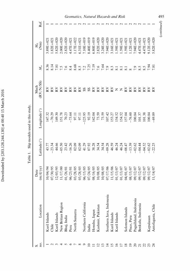
Table1.
Slipmodelsusedin
thisstudy.
S.
no.
Location
Date
(m6d
6yy)
Latitude(�)
Longitude(�)
Mech
(RV6N
6SS)
Mw
M0
(Nm)
Ref.
1KurilIslands
10604694
43.77
147.32
RV
8.36
3.89EC0
21
1
2Chile
07630695
¡23.34
¡70.29
RV
8.14
1.82EC0
21
1
3KurilIslands
12603695
44.66
149.30
RV
7.81
5.82EC0
20
1
4New
BritianRegion
11617600
¡05.50
151.78
RV
7.5
2.00EC0
20
1
5Bhuj,India
01626601
23.42
70.23
RV
7.6
2.82EC0
20
2
6Peru
06623601
¡16.26
¡73.64
RV
8.4
4.47EC0
21
1
7NorthSumatra
03628605
02.09
97.11
RV
8.68
1.17EC0
22
1
803628605
02.09
97.11
RV
8.5
6.31EC0
21
2
9NorthernCalifornia
06615605
41.29
¡125.95
SS
7.2
7.10EC0
19
2
10
India
07624605
07.92
92.19
SS
7.25
8.40EC0
19
1
11
Honshu,Japan
08616605
38.28
142.04
RV
7.19
6.80EC0
19
1
12
Kashmir,Pakistan
10608605
34.54
73.59
RV
7.6
2.82EC0
20
2
13
10608605
34.54
73.59
RV
7.64
3.24EC0
20
1
14
SouthernJava,Indonesia
07617606
¡09.28
107.42
RV
7.9
7.94EC0
20
2
15
KurilIslands
11615606
46.59
153.27
RV
8.3
3.16EC0
21
2
16
KurilIslands
01613607
46.24
154.52
N8.1
1.59EC0
21
1
17
01613607
46.24
154.52
N8.1
1.59EC0
21
2
18
SolomonIslands
04601607
¡08.47
157.04
RV
8.1
1.59EC0
21
1
19
Pisco,Peru
08615607
¡13.39
¡76.60
RV
81.12EC0
21
2
20
PagaiIsland,Indonesia
09612607
¡02.62
100.84
RV
7.9
7.94EC0
20
2
21
Benkulu,Indonesia
09612607
¡04.44
101.37
RV
8.5
4.47EC0
21
2
22
09612607
¡04.52
101.38
RV
8.5
4.47EC0
21
1
23
Kepulauan
09612607
¡02.62
100.84
RV
7.94
9.12EC0
20
1
24
Antofagasta,Chile
11614607
¡22.25
¡69.89
RV
7.81
5.82EC0
20
1
( continued
)
Geomatics, Natural Hazards and Risk 495
Dow
nloa
ded
by [
203.
128.
244.
130]
at 0
0:40
15
Mar
ch 2
016
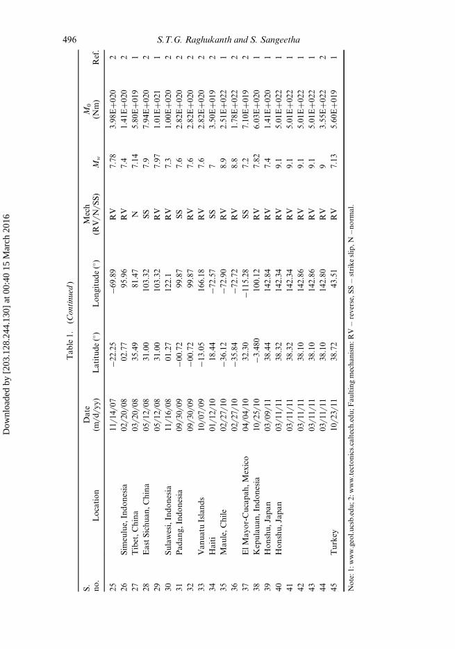
Table1.
(Continued
)
S.
no.
Location
Date
(m6d
6yy)
Latitude(�)
Longitude(�)
Mech
(RV6N
6SS)
Mw
M0
(Nm)
Ref.
25
11614607
¡22.25
¡69.89
RV
7.78
3.98EC0
20
2
26
Sim
eulue,Indonesia
02620608
02.77
95.96
RV
7.4
1.41EC0
20
2
27
Tibet,China
03620608
35.49
81.47
N7.14
5.80EC0
19
1
28
EastSichuan,China
05612608
31.00
103.32
SS
7.9
7.94EC0
20
2
29
05612608
31.00
103.32
RV
7.97
1.01EC0
21
1
30
Sulawesi,Indonesia
11616608
01.27
122.1
RV
7.3
1.00EC0
20
2
31
Padang,Indonesia
09630609
¡00.72
99.87
SS
7.6
2.82EC0
20
2
32
09630609
¡00.72
99.87
RV
7.6
2.82EC0
20
2
33
Vanuatu
Islands
10607609
¡13.05
166.18
RV
7.6
2.82EC0
20
2
34
Haiti
01612610
18.44
¡72.57
SS
73.50EC0
19
2
35
Maule,Chile
02627610
¡36.12
¡72.90
RV
8.9
2.51EC0
22
1
36
02627610
¡35.84
¡72.72
RV
8.8
1.78EC0
22
2
37
ElMayor-Cucapah,Mexico
04604610
32.30
¡115.28
SS
7.2
7.10EC0
19
2
38
Kepulauan,Indonesia
10625610
¡3.480
100.12
RV
7.82
6.03EC0
20
1
39
Honshu,Japan
03609611
38.44
142.84
RV
7.4
1.41EC0
20
1
40
Honshu,Japan
03611611
38.32
142.34
RV
9.1
5.01EC0
22
1
41
03611611
38.32
142.34
RV
9.1
5.01EC0
22
1
42
03611611
38.10
142.86
RV
9.1
5.01EC0
22
1
43
03611611
38.10
142.86
RV
9.1
5.01EC0
22
1
44
03611611
38.10
142.80
RV
93.55EC0
22
2
45
Turkey
10623611
38.72
43.51
RV
7.13
5.60EC0
19
1
Note:1:www.geol.ucsb.edu;2:www.tectonics.caltech.edu;Faultingmechanism:RV�
reverse,SS�
strikeslip,N
�norm
al.
496 S.T.G. Raghukanth and S. Sangeetha
Dow
nloa
ded
by [
203.
128.
244.
130]
at 0
0:40
15
Mar
ch 2
016
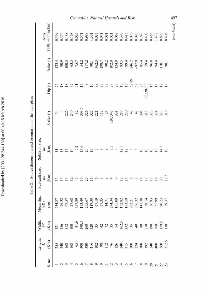
Table2.
Sourcedim
ensionsandorientationofthefaultplane.
Length,
LWidth,
WMeanslip,
<D>
Subfaultsize,
dx
SubfaultSize,
dz
S.no.
(Km)
(Km)
(cm)
(Km)
(Km)
Strike(�)
Dip
(�)
Rake(�)
Area
(1.0EC0
5�sq.km)
1255
121
234.87
15
11
54
76
123.4
0.309
2240
156
96.32
15
13
418
90.9
0.374
3168
112
67.57
14
14
226
18
100.3
0.188
4168
100
27.68
12
10
240
32
63.5
0.168
565
41.6
357.89
55.2
82
51
75.7
0.027
6300
190.4
173.49
15
13.6
308.5
15
54.2
0.571
7380
260
255.67
20
20
326
8117.2
0.988
8416
320
119.38
16
16
325
10
90.1
1.331
9102
35
67.19
65
221
88
362.3
0.036
10
98
42
67.35
77
118
80
198.7
0.041
11
112
72
14.71
88
24
70
90.2
0.081
12
76
35
294.34
43.5
3206343
29
102.9
0.021
13
126
54
175.09
99
331
29
124.9
0.068
14
240
162.5
152.82
12
12.5
289
10
83.5
0.390
15
315
132
173.59
15
12
220
15
99.4
0.416
16
200
35
702.21
85
42
57.89
246.2
0.070
17
224
40
356.32
85
42
58
¡97.9
0.090
18
300
80
147.38
15
10
305
25
85.4
0.240
19
192
210
58.14
12
10
318
06620630
59.4
0.403
20
240
190
36.93
12
10
323
15
96.8
0.456
21
400
368
55.99
16
16
324
15
94.4
1.472
22
560
159.5
90.23
20
14.5
323
12
110.1
0.893
23
312.5
130
39.37
12.5
10
319
19
98.1
0.406
(continued
)
Geomatics, Natural Hazards and Risk 497
Dow
nloa
ded
by [
203.
128.
244.
130]
at 0
0:40
15
Mar
ch 2
016
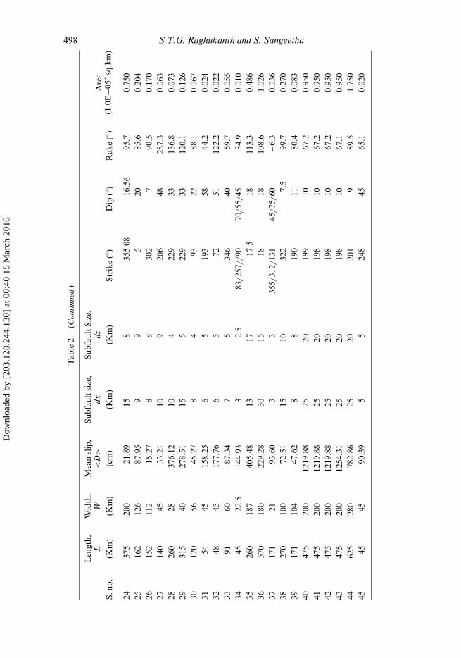
Table2.
(Continued
)
Length,
LWidth,
WMeanslip,
<D>
Subfaultsize,
dx
SubfaultSize,
dz
S.no.
(Km)
(Km)
(cm)
(Km)
(Km)
Strike(�)
Dip
(�)
Rake(�)
Area
(1.0EC0
5�sq.km)
24
375
200
21.89
15
8355.08
16.56
95.7
0.750
25
162
126
87.95
99
520
85.6
0.204
26
152
112
15.27
88
302
790.5
0.170
27
140
45
33.21
10
9206
48
287.3
0.063
28
260
28
376.12
10
4229
33
136.8
0.073
29
315
40
278.51
15
5229
33
120.1
0.126
30
120
56
45.27
84
93
22
88.1
0.067
31
54
45
158.25
65
193
58
44.2
0.024
32
48
45
177.76
65
72
51
122.2
0.022
33
91
60
87.34
75
346
40
59.7
0.055
34
45
22.5
144.93
32.5
83625766
90
70655645
34.9
0.010
35
260
187
405.48
13
17
17.5
18
113.3
0.486
36
570
180
229.28
30
15
18
18
108.6
1.026
37
171
21
93.60
33
35563126131
45675660
¡6.3
0.036
38
270
100
72.51
15
10
322
7.5
99.7
0.270
39
171
104
47.62
88
190
11
80.4
0.083
40
475
200
1219.88
25
20
199
10
67.2
0.950
41
475
200
1219.88
25
20
198
10
67.2
0.950
42
475
200
1219.88
25
20
198
10
67.2
0.950
43
475
200
1254.31
25
20
198
10
67.1
0.950
44
625
280
782.86
25
20
201
989.5
1.750
45
45
45
90.39
55
248
45
65.1
0.020
498 S.T.G. Raghukanth and S. Sangeetha
Dow
nloa
ded
by [
203.
128.
244.
130]
at 0
0:40
15
Mar
ch 2
016
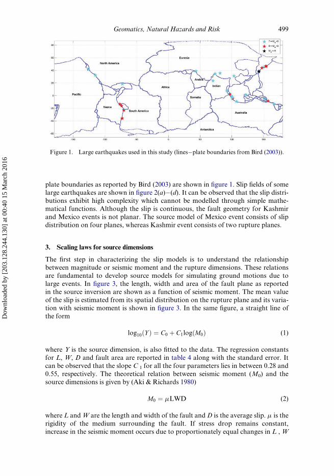
plate boundaries as reported by Bird (2003) are shown in figure 1. Slip fields of some
large earthquakes are shown in figure 2(a)�(d). It can be observed that the slip distri-
butions exhibit high complexity which cannot be modelled through simple mathe-matical functions. Although the slip is continuous, the fault geometry for Kashmir
and Mexico events is not planar. The source model of Mexico event consists of slip
distribution on four planes, whereas Kashmir event consists of two rupture planes.
3. Scaling laws for source dimensions
The first step in characterizing the slip models is to understand the relationship
between magnitude or seismic moment and the rupture dimensions. These relations
are fundamental to develop source models for simulating ground motions due to
large events. In figure 3, the length, width and area of the fault plane as reported
in the source inversion are shown as a function of seismic moment. The mean value
of the slip is estimated from its spatial distribution on the rupture plane and its varia-
tion with seismic moment is shown in figure 3. In the same figure, a straight line of
the form
log10ðY Þ ¼ C0 þ C1logðM0Þ (1)
where Y is the source dimension, is also fitted to the data. The regression constants
for L, W, D and fault area are reported in table 4 along with the standard error. It
can be observed that the slope C 1 for all the four parameters lies in between 0.28 and
0.55, respectively. The theoretical relation between seismic moment (M0) and the
source dimensions is given by (Aki & Richards 1980)
M0 ¼ mLWD (2)
where L andW are the length and width of the fault andD is the average slip. m is the
rigidity of the medium surrounding the fault. If stress drop remains constant,
increase in the seismic moment occurs due to proportionately equal changes in L , W
Figure 1. Large earthquakes used in this study (lines�plate boundaries from Bird (2003)).
Geomatics, Natural Hazards and Risk 499
Dow
nloa
ded
by [
203.
128.
244.
130]
at 0
0:40
15
Mar
ch 2
016
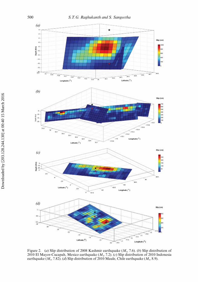
Figure 2. (a) Slip distribution of 2008 Kashmir earthquake (Mw 7.6). (b) Slip distribution of2010 El Mayor-Cucapah, Mexico earthquake (Mw 7.2). (c) Slip distribution of 2010 Indonesiaearthquake (Mw 7.82). (d) Slip distribution of 2010 Maule, Chile earthquake (Mw 8.9).
500 S.T.G. Raghukanth and S. Sangeetha
Dow
nloa
ded
by [
203.
128.
244.
130]
at 0
0:40
15
Mar
ch 2
016
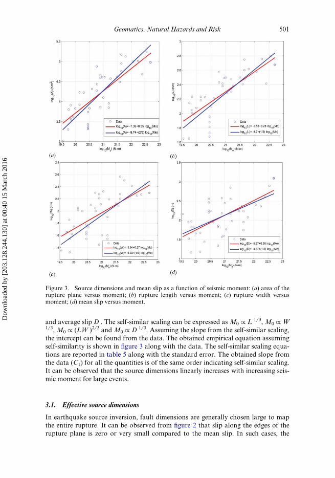
and average slip D . The self-similar scaling can be expressed as M0 / L 16 3, M0 / W16 3, M0 / (LW )26 3 and M0 / D 16 3. Assuming the slope from the self-similar scaling,
the intercept can be found from the data. The obtained empirical equation assuming
self-similarity is shown in figure 3 along with the data. The self-similar scaling equa-
tions are reported in table 5 along with the standard error. The obtained slope from
the data (C1) for all the quantities is of the same order indicating self-similar scaling.
It can be observed that the source dimensions linearly increases with increasing seis-
mic moment for large events.
3.1. Effective source dimensions
In earthquake source inversion, fault dimensions are generally chosen large to map
the entire rupture. It can be observed from figure 2 that slip along the edges of the
rupture plane is zero or very small compared to the mean slip. In such cases, the
Figure 3. Source dimensions and mean slip as a function of seismic moment: (a) area of therupture plane versus moment; (b) rupture length versus moment; (c) rupture width versusmoment; (d) mean slip versus moment.
Geomatics, Natural Hazards and Risk 501
Dow
nloa
ded
by [
203.
128.
244.
130]
at 0
0:40
15
Mar
ch 2
016
length and the width of the reported slip models will overestimate the true rupturedimensions. Estimating the exact source dimension from the slip distribution is diffi-
cult. To circumvent this problem, there have been techniques developed based on
empirical approaches. Somerville et al. (1999) defined the rupture dimensions based
on the slip distribution. If the slip distribution along the edges of the fault is 0.3 times
less than the average slip, the entire row or the column is removed from the rupture
distribution. Mai and Beroza (2000) defined the effective source dimensions based on
autocorrelation function. To estimate the effective length and width, marginal slip
distributions are derived by summing the slip in both the along-strike and down-dipdirections. The autocorrelation function is estimated and the width of this function is
computed as (Bracewell 1986)
Wa ¼ 1
D�Dj0
Z 1
¡1D�Ddx (3)
where Wa is the autocorrelation width and � is the convolution operator. The effec-
tive length and width of the rupture plane are estimated from the marginal slip distri-
bution in along- strike and down-dip directions. In a similar fashion, effective lengthand width have been estimated for all the slip models. These are reported in table 3
for all the 45 slip models. In figure 4, a comparison between the effective area and
the area of fault dimensions used in the earthquake source inversion is shown. The
ratio between effective dimensions to original dimensions has been estimated. The
ratio between effective length to original length lies in between 0.51 and 0.95 with a
median value of 0.74. In down-dip direction, the median change in width is 0.76 and
it lies in between 0.43 and 0.96 for all the 45 rupture models used in this analysis. The
effective area of all the events lies in between 24% and 88% of the original sourcedimensions. Empirical equations to predict effective source dimensions from seismic
moment are derived from the data. The coefficients are reported in table 4. The fitted
equations are shown along with the data in figure 5. The self-similar scaling relations
by constraining the slope are also shown in figure 5. The effective source dimensions
increase with increase in the seismic moment. Since the effective area is less than the
original source dimensions, the slip on the fault plane has to be increased to conserve
the seismic moment. The average effective slip variation with moment is shown in
figure 5(d). The standard deviation around the mean value also increases withincrease in the seismic moment.
4. Asperities on the rupture plane
After deriving the equations for estimating the source dimensions, the next step is to
understand the regions of concentration of large slip relative to the mean slip on therupture plane. These regions are known as asperities. There is no guideline available
to determine the threshold value of slip to define an asperity. The approaches in the
literature have been empirical and based on personal judgement. Somerville et al.
(1999) define asperities as rectangular regions whose average slip is 1.5 times more
than the mean slip on the entire rupture plane. In this study, the approach of Mai
et al. (2005) based on the ratio of slip distribution on the rupture plane to the maxi-
mum slip is used to define asperities. The subfaults on which the ratio lies in between
0.33 � D6 Dmax � 0.66 are taken as large asperity. The regions where the ratio
502 S.T.G. Raghukanth and S. Sangeetha
Dow
nloa
ded
by [
203.
128.
244.
130]
at 0
0:40
15
Mar
ch 2
016
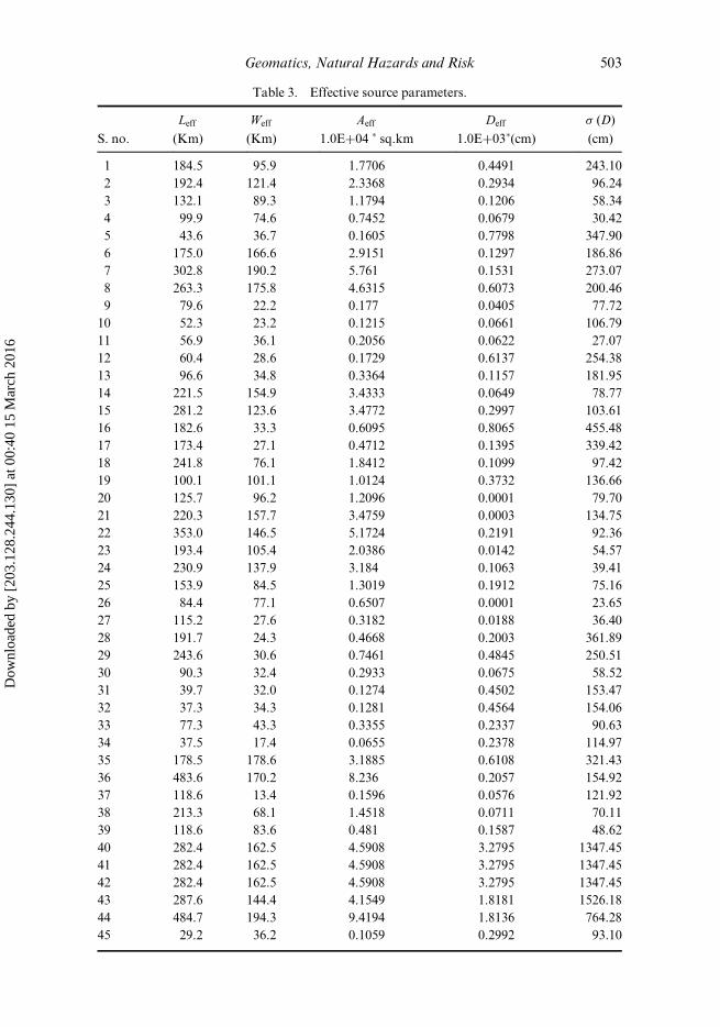
Table 3. Effective source parameters.
Leff Weff Aeff Deff s (D)
S. no. (Km) (Km) 1.0EC04 � sq.km 1.0EC03�(cm) (cm)
1 184.5 95.9 1.7706 0.4491 243.10
2 192.4 121.4 2.3368 0.2934 96.24
3 132.1 89.3 1.1794 0.1206 58.34
4 99.9 74.6 0.7452 0.0679 30.42
5 43.6 36.7 0.1605 0.7798 347.90
6 175.0 166.6 2.9151 0.1297 186.86
7 302.8 190.2 5.761 0.1531 273.07
8 263.3 175.8 4.6315 0.6073 200.46
9 79.6 22.2 0.177 0.0405 77.72
10 52.3 23.2 0.1215 0.0661 106.79
11 56.9 36.1 0.2056 0.0622 27.07
12 60.4 28.6 0.1729 0.6137 254.38
13 96.6 34.8 0.3364 0.1157 181.95
14 221.5 154.9 3.4333 0.0649 78.77
15 281.2 123.6 3.4772 0.2997 103.61
16 182.6 33.3 0.6095 0.8065 455.48
17 173.4 27.1 0.4712 0.1395 339.42
18 241.8 76.1 1.8412 0.1099 97.42
19 100.1 101.1 1.0124 0.3732 136.66
20 125.7 96.2 1.2096 0.0001 79.70
21 220.3 157.7 3.4759 0.0003 134.75
22 353.0 146.5 5.1724 0.2191 92.36
23 193.4 105.4 2.0386 0.0142 54.57
24 230.9 137.9 3.184 0.1063 39.41
25 153.9 84.5 1.3019 0.1912 75.16
26 84.4 77.1 0.6507 0.0001 23.65
27 115.2 27.6 0.3182 0.0188 36.40
28 191.7 24.3 0.4668 0.2003 361.89
29 243.6 30.6 0.7461 0.4845 250.51
30 90.3 32.4 0.2933 0.0675 58.52
31 39.7 32.0 0.1274 0.4502 153.47
32 37.3 34.3 0.1281 0.4564 154.06
33 77.3 43.3 0.3355 0.2337 90.63
34 37.5 17.4 0.0655 0.2378 114.97
35 178.5 178.6 3.1885 0.6108 321.43
36 483.6 170.2 8.236 0.2057 154.92
37 118.6 13.4 0.1596 0.0576 121.92
38 213.3 68.1 1.4518 0.0711 70.11
39 118.6 83.6 0.481 0.1587 48.62
40 282.4 162.5 4.5908 3.2795 1347.45
41 282.4 162.5 4.5908 3.2795 1347.45
42 282.4 162.5 4.5908 3.2795 1347.45
43 287.6 144.4 4.1549 1.8181 1526.18
44 484.7 194.3 9.4194 1.8136 764.28
45 29.2 36.2 0.1059 0.2992 93.10
Geomatics, Natural Hazards and Risk 503
Dow
nloa
ded
by [
203.
128.
244.
130]
at 0
0:40
15
Mar
ch 2
016
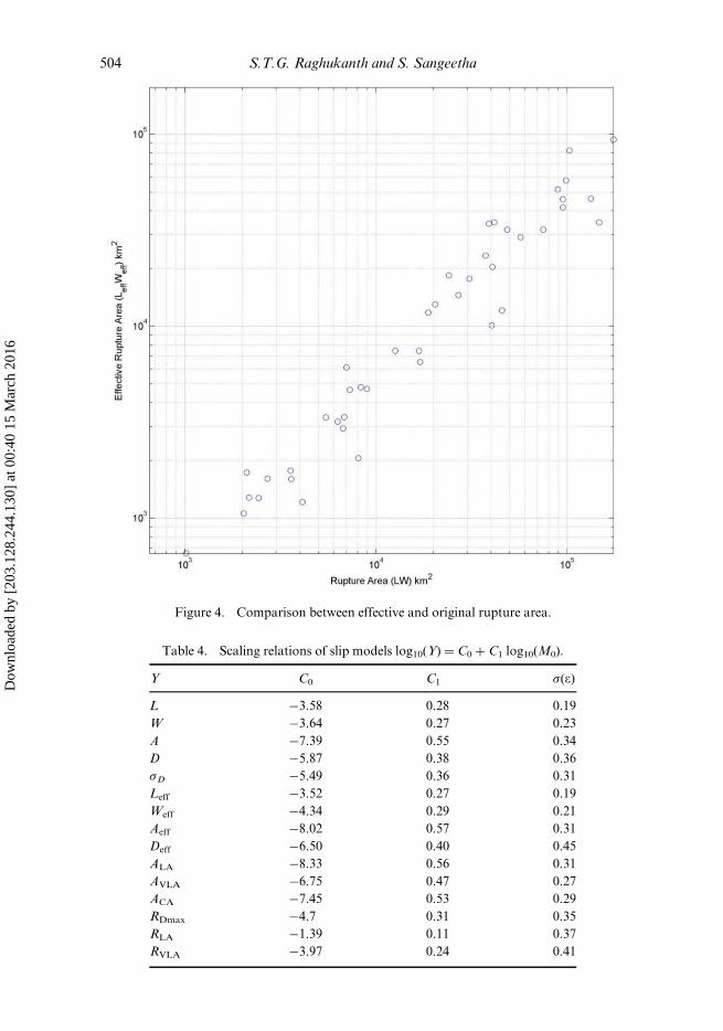
Figure 4. Comparison between effective and original rupture area.
Table 4. Scaling relations of slip models log10(Y) D C0 C C1 log10(M0).
Y C0 C1 s(e)
L ¡3.58 0.28 0.19
W ¡3.64 0.27 0.23
A ¡7.39 0.55 0.34
D ¡5.87 0.38 0.36
sD ¡5.49 0.36 0.31
Leff ¡3.52 0.27 0.19
Weff ¡4.34 0.29 0.21
Aeff ¡8.02 0.57 0.31
Deff ¡6.50 0.40 0.45
ALA ¡8.33 0.56 0.31
AVLA ¡6.75 0.47 0.27
ACA ¡7.45 0.53 0.29
RDmax ¡4.7 0.31 0.35
RLA ¡1.39 0.11 0.37
RVLA ¡3.97 0.24 0.41
504 S.T.G. Raghukanth and S. Sangeetha
Dow
nloa
ded
by [
203.
128.
244.
130]
at 0
0:40
15
Mar
ch 2
016
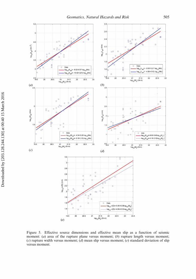
Figure 5. Effective source dimensions and effective mean slip as a function of seismicmoment: (a) area of the rupture plane versus moment; (b) rupture length versus moment;(c) rupture width versus moment; (d) mean slip versus moment; (e) standard deviation of slipversus moment.
Geomatics, Natural Hazards and Risk 505
Dow
nloa
ded
by [
203.
128.
244.
130]
at 0
0:40
15
Mar
ch 2
016
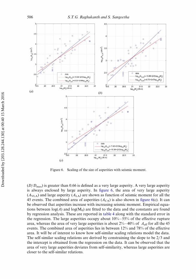
(D6 Dmax) is greater than 0.66 is defined as a very large asperity. A very large asperity
is always enclosed by large asperity. In figure 6, the area of very large asperity
(AVLA) and large asperity (ALA) are shown as function of seismic moment for all the
45 events. The combined area of asperities (ACA) is also shown in figure 6(c). It can
be observed that asperities increase with increasing seismic moment. Empirical equa-
tions between log(A) and log(M0) are fitted to the data and the constants are foundby regression analysis. These are reported in table 4 along with the standard error in
the regression. The large asperities occupy about 10%�55% of the effective rupture
area, whereas the area of very large asperities is about 2%�40% of Aeff for all the 45
events. The combined area of asperities lies in between 12% and 78% of the effective
area. It will be of interest to know how self-similar scaling relations model the data.
The self-similar scaling relations are derived by constraining the slope to be 26 3 and
the intercept is obtained from the regression on the data. It can be observed that the
area of very large asperities deviates from self-similarity, whereas large asperities arecloser to the self-similar relations.
Figure 6. Scaling of the size of asperities with seismic moment.
506 S.T.G. Raghukanth and S. Sangeetha
Dow
nloa
ded
by [
203.
128.
244.
130]
at 0
0:40
15
Mar
ch 2
016
4.1. Location of hypocentre and asperities
Another important aspect which affects the near-field ground motion is the location of
hypocentre and asperities on the fault plane. This information is important to under-
stand the crack propagation during the rupture which can be further used to developdynamic rupture models. The distance of the hypocentre from the edges of the fault in
along-strike (Hx ) and down-dip (Hz ) directions normalized by length and width of the
fault is computed for all the 45 slip models. Due to symmetry, the normalized distance in
along-strike direction (Hx ) lies in between 0 and 0.5, whereasHz lies in between 0 and 1.
Hx D 0 indicates that hypocentre is located on the edge of the fault, whereas Hx D 0.5
indicates the centre of the fault. Similarly,HzD 0 denotes the hypocentral location at the
top edge of the fault and Hz D 1 denotes the bottom edge of the rupture plane. These
non-dimensional quantities are shown in figure 7 as a function of magnitude. It can beobserved that Hx and Hz do not show any pattern with Mw. The histograms are also
shown in figure 7. The Hx is distributed with a mean of 0.30 and a standard deviation
0.13, whereas forHz, these two moments are 0.52 and 0.23, respectively. The hypocentre
is approximately located at the centre of the fault in down-dip direction.
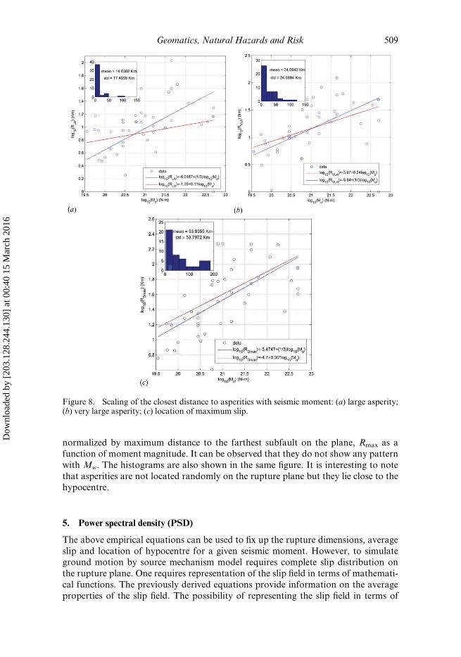
To understand the relationship between the hypocentre and the location of the
asperity, the closest distance to the asperity from the hypocentre is determined from
the data. In figure 8, the variation of the closest distance to large and very large
asperities from hypocentre is shown as a function of seismic moment. The histogramsof these distances are also shown in the same figure. The closest distance increases
with increase in the seismic moment. Large asperities are located close to the hypo-
centre, whereas very large asperities are located at approximately 24 km from the
hypocentre. The regions of maximum slip are located approximately at a distance of
50 km from the hypocentre. Empirical equations between distance and moment are
derived from the data with and without constraining the slope, and constants are
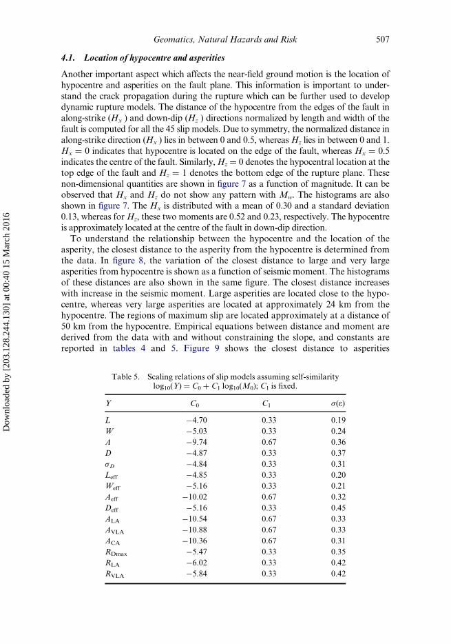
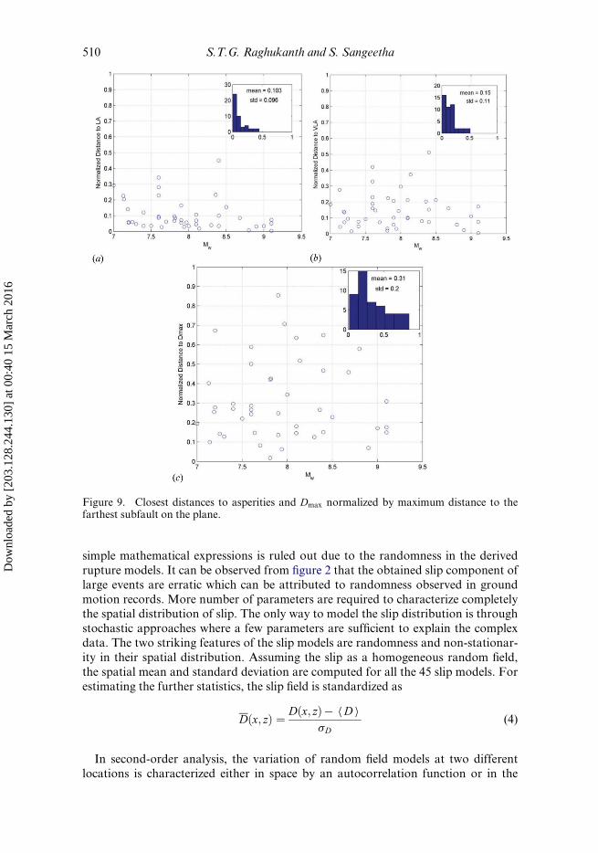
reported in tables 4 and 5. Figure 9 shows the closest distance to asperities
Table 5. Scaling relations of slip models assuming self-similaritylog10(Y) D C0 C C1 log10(M0); C1 is fixed.
Y C0 C1 s(e)
L ¡4.70 0.33 0.19
W ¡5.03 0.33 0.24
A ¡9.74 0.67 0.36
D ¡4.87 0.33 0.37
sD ¡4.84 0.33 0.31
Leff ¡4.85 0.33 0.20
Weff ¡5.16 0.33 0.21
Aeff ¡10.02 0.67 0.32
Deff ¡5.16 0.33 0.45
ALA ¡10.54 0.67 0.33
AVLA ¡10.88 0.67 0.33
ACA ¡10.36 0.67 0.31
RDmax ¡5.47 0.33 0.35
RLA ¡6.02 0.33 0.42
RVLA ¡5.84 0.33 0.42
Geomatics, Natural Hazards and Risk 507
Dow
nloa
ded
by [
203.
128.
244.
130]
at 0
0:40
15
Mar
ch 2
016
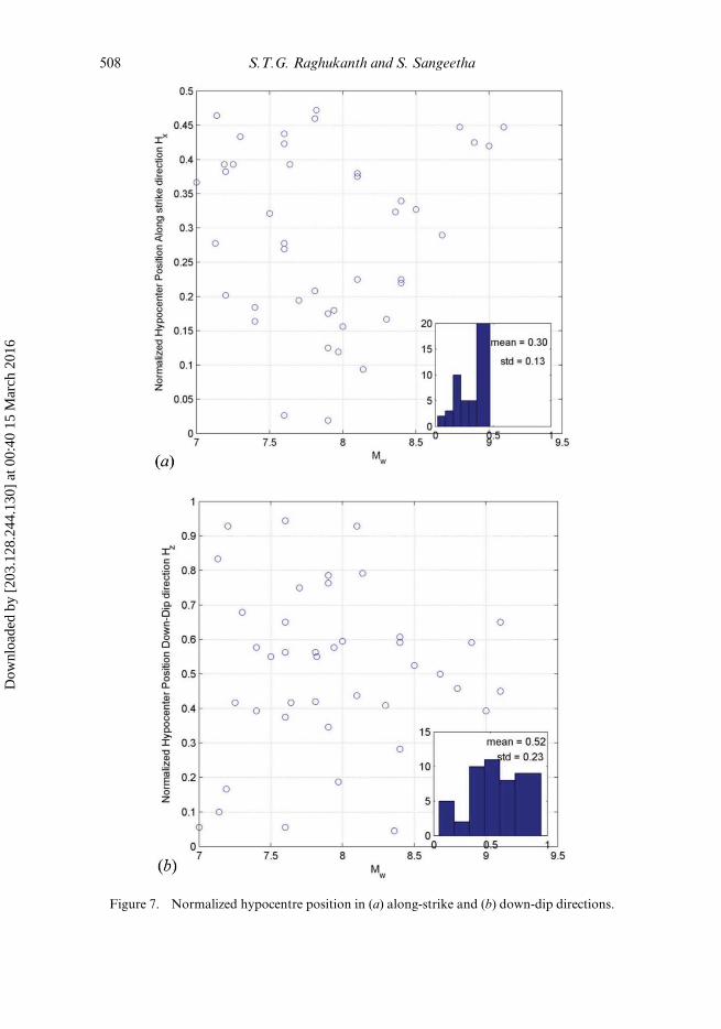
Figure 7. Normalized hypocentre position in (a) along-strike and (b) down-dip directions.
508 S.T.G. Raghukanth and S. Sangeetha
Dow
nloa
ded
by [
203.
128.
244.
130]
at 0
0:40
15
Mar
ch 2
016
normalized by maximum distance to the farthest subfault on the plane, Rmax as a
function of moment magnitude. It can be observed that they do not show any pattern
with Mw. The histograms are also shown in the same figure. It is interesting to note
that asperities are not located randomly on the rupture plane but they lie close to thehypocentre.
5. Power spectral density (PSD)
The above empirical equations can be used to fix up the rupture dimensions, average
slip and location of hypocentre for a given seismic moment. However, to simulate
ground motion by source mechanism model requires complete slip distribution on
the rupture plane. One requires representation of the slip field in terms of mathemati-
cal functions. The previously derived equations provide information on the average
properties of the slip field. The possibility of representing the slip field in terms of
Figure 8. Scaling of the closest distance to asperities with seismic moment: (a) large asperity;(b) very large asperity; (c) location of maximum slip.
Geomatics, Natural Hazards and Risk 509
Dow
nloa
ded
by [
203.
128.
244.
130]
at 0
0:40
15
Mar
ch 2
016
simple mathematical expressions is ruled out due to the randomness in the derived
rupture models. It can be observed from figure 2 that the obtained slip component of
large events are erratic which can be attributed to randomness observed in ground
motion records. More number of parameters are required to characterize completelythe spatial distribution of slip. The only way to model the slip distribution is through
stochastic approaches where a few parameters are sufficient to explain the complex
data. The two striking features of the slip models are randomness and non-stationar-
ity in their spatial distribution. Assuming the slip as a homogeneous random field,
the spatial mean and standard deviation are computed for all the 45 slip models. For
estimating the further statistics, the slip field is standardized as
Dðx; zÞ ¼ Dðx; zÞ¡ hD isD
(4)
In second-order analysis, the variation of random field models at two different
locations is characterized either in space by an autocorrelation function or in the
Figure 9. Closest distances to asperities and Dmax normalized by maximum distance to thefarthest subfault on the plane.
510 S.T.G. Raghukanth and S. Sangeetha
Dow
nloa
ded
by [
203.
128.
244.
130]
at 0
0:40
15
Mar
ch 2
016
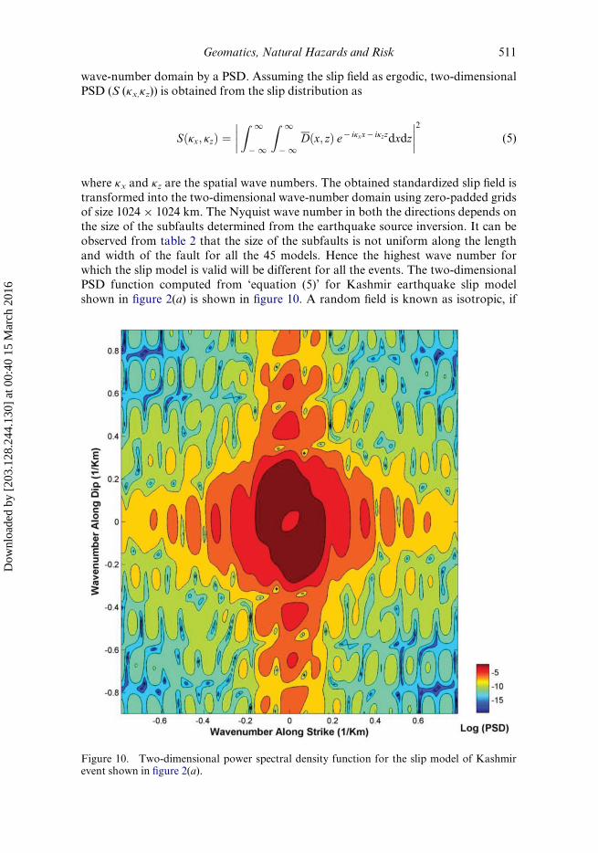
wave-number domain by a PSD. Assuming the slip field as ergodic, two-dimensionalPSD (S (kx,kz)) is obtained from the slip distribution as
Sðkx; kzÞ ¼����Z 1
¡ 1
Z 1
¡ 1Dðx; zÞ e¡ ikxx¡ ikzzdxdz
����2
(5)
where kx and kz are the spatial wave numbers. The obtained standardized slip field is
transformed into the two-dimensional wave-number domain using zero-padded gridsof size 1024 £ 1024 km. The Nyquist wave number in both the directions depends on
the size of the subfaults determined from the earthquake source inversion. It can be
observed from table 2 that the size of the subfaults is not uniform along the length
and width of the fault for all the 45 models. Hence the highest wave number for
which the slip model is valid will be different for all the events. The two-dimensional
PSD function computed from ‘equation (5)’ for Kashmir earthquake slip model
shown in figure 2(a) is shown in figure 10. A random field is known as isotropic, if
Figure 10. Two-dimensional power spectral density function for the slip model of Kashmirevent shown in figure 2(a).
Geomatics, Natural Hazards and Risk 511
Dow
nloa
ded
by [
203.
128.
244.
130]
at 0
0:40
15
Mar
ch 2
016
the correlation is independent of direction (Vanmarcke 1983). It can observed fromfigure 10 that the correlation structure is different in along-strike and dip-directions
indicating that the moment field is anisotropic. In figure 11, the PSD functions at
cross sections kx D 0 and kz D 0 are also shown. There are several theoretical two-
dimensional correlation functions available in the literature. Three correlation func-
tions widely used in literature are Gaussian, exponential and von Karman (Mai &
Beroza 2002). The expressions for the autocorrelation and PSD for these three ran-
dom field models are as follows:
Gaussian:
Rðzx; zzÞ ¼ e¡ z2x
a2x
þz2z
a2z
� �Sðkx; kzÞ ¼ axaz
2e¡ 1
4ða2xk2xþa2z k
2z Þ (6)
Exponential:
Rðzx; zzÞ ¼ e¡
ffiffiffiffiffiffiffiffiffiz2x
a2x
þz2z
a2z
qSðkx; kzÞ ¼ axaz
ð1þ a2xk2x þ a2zk
2z Þ
32
(7)
von Karman:
Rðzx; zzÞ ¼GH ðrÞGHð0Þ Sðkx; kzÞ ¼ axaz
ð1þ a2xk2x þ a2zk
2z ÞHþ1
(8)
where
GH ðrÞ ¼ rHKHðrÞ r ¼ffiffiffiffiffiffiffiffiffiffiffiffiffiffiffiz2xa2x
þ z2za2z
s(9)
ax and az are the correlation lengths along x and z-directions, respectively. H is the
Hurst exponent and KH is the modified Bessel function of the first kind. It can be
observed that when H D 0.5 von Karman is identical to the exponential PSD. The
parameters ax and az of the three random fields are estimated from the slip field by
minimizing the mean square error between the computed PSD and the expressionsshown in equations (6)�(8). The fitted Gaussian, exponential and von Karman PSD
at cross sections kx D 0 and kz D 0 are plotted in figure 11 along with the data for
Kashmir earthquake. Besides, the estimated parameters are also shown in the same
figure. The misfit associated with von Karman function is slightly lower than that
obtained from exponential and Gaussian function, and hence the slip fluctuation can
be modelled as a von Karman random field. Similarly, the correlation lengths are
estimated for all the slip models. These are reported in table 6 for Gaussian, exponen-
tial and von Karman PSD. The correlation length ax is much larger than az whichcan be attributed to large length compared to the width of the fault.
6. Scaling laws for correlation lengths
After estimating the spectral parameters from PSD, it remains to identify the pat-
terns with the previous determined effective source dimensions and moment
512 S.T.G. Raghukanth and S. Sangeetha
Dow
nloa
ded
by [
203.
128.
244.
130]
at 0
0:40
15
Mar
ch 2
016
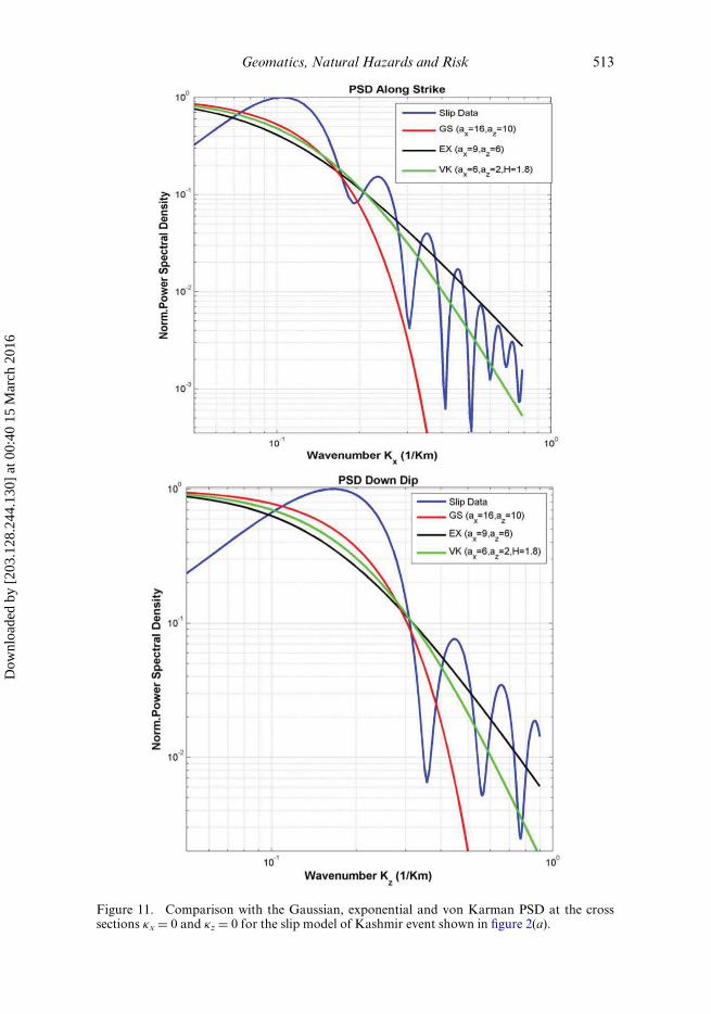
Figure 11. Comparison with the Gaussian, exponential and von Karman PSD at the crosssections kx D 0 and kz D 0 for the slip model of Kashmir event shown in figure 2(a).
Geomatics, Natural Hazards and Risk 513
Dow
nloa
ded
by [
203.
128.
244.
130]
at 0
0:40
15
Mar
ch 2
016
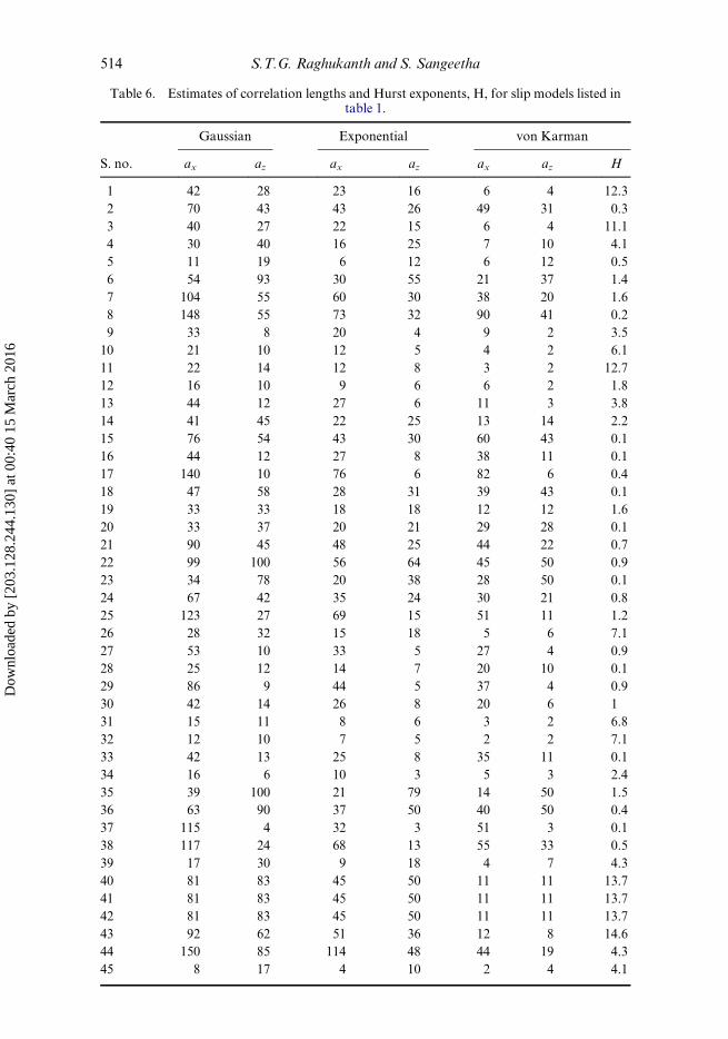
Table 6. Estimates of correlation lengths and Hurst exponents, H, for slip models listed intable 1.
Gaussian Exponential von Karman
S. no. ax az ax az ax az H
1 42 28 23 16 6 4 12.3
2 70 43 43 26 49 31 0.3
3 40 27 22 15 6 4 11.1
4 30 40 16 25 7 10 4.1
5 11 19 6 12 6 12 0.5
6 54 93 30 55 21 37 1.4
7 104 55 60 30 38 20 1.6
8 148 55 73 32 90 41 0.2
9 33 8 20 4 9 2 3.5
10 21 10 12 5 4 2 6.1
11 22 14 12 8 3 2 12.7
12 16 10 9 6 6 2 1.8
13 44 12 27 6 11 3 3.8
14 41 45 22 25 13 14 2.2
15 76 54 43 30 60 43 0.1
16 44 12 27 8 38 11 0.1
17 140 10 76 6 82 6 0.4
18 47 58 28 31 39 43 0.1
19 33 33 18 18 12 12 1.6
20 33 37 20 21 29 28 0.1
21 90 45 48 25 44 22 0.7
22 99 100 56 64 45 50 0.9
23 34 78 20 38 28 50 0.1
24 67 42 35 24 30 21 0.8
25 123 27 69 15 51 11 1.2
26 28 32 15 18 5 6 7.1
27 53 10 33 5 27 4 0.9
28 25 12 14 7 20 10 0.1
29 86 9 44 5 37 4 0.9
30 42 14 26 8 20 6 1
31 15 11 8 6 3 2 6.8
32 12 10 7 5 2 2 7.1
33 42 13 25 8 35 11 0.1
34 16 6 10 3 5 3 2.4
35 39 100 21 79 14 50 1.5
36 63 90 37 50 40 50 0.4
37 115 4 32 3 51 3 0.1
38 117 24 68 13 55 33 0.5
39 17 30 9 18 4 7 4.3
40 81 83 45 50 11 11 13.7
41 81 83 45 50 11 11 13.7
42 81 83 45 50 11 11 13.7
43 92 62 51 36 12 8 14.6
44 150 85 114 48 44 19 4.3
45 8 17 4 10 2 4 4.1
514 S.T.G. Raghukanth and S. Sangeetha
Dow
nloa
ded
by [
203.
128.
244.
130]
at 0
0:40
15
Mar
ch 2
016
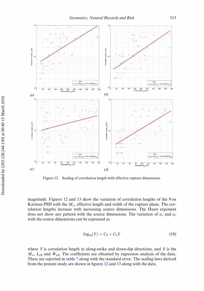
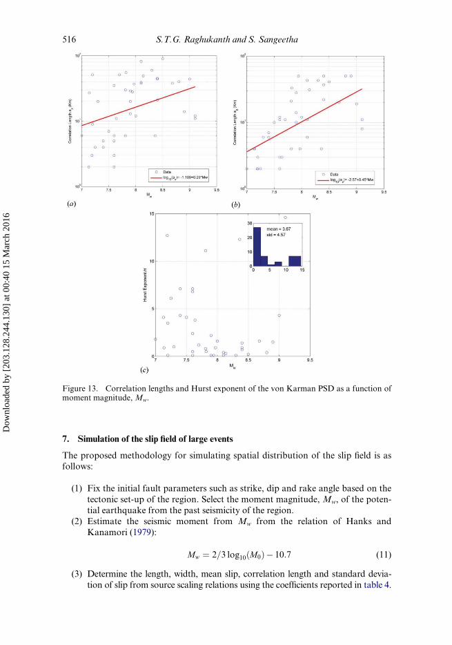
magnitude. Figures 12 and 13 show the variation of correlation lengths of the Von
Karman PSD with the Mw, effective length and width of the rupture plane. The cor-
relation lengths increase with increasing source dimensions. The Hurst exponent
does not show any pattern with the source dimensions. The variation of ax and azwith the source dimensions can be expressed as
log10ðY Þ ¼ C0 þ C1X (10)
where Y is correlation length in along-strike and down-dip directions, and X is the
Mw, Leff and Weff. The coefficients are obtained by regression analysis of the data.
These are reported in table 7 along with the standard error. The scaling laws derived
from the present study are shown in figures 12 and 13 along with the data.
Figure 12. Scaling of correlation length with effective rupture dimensions.
Geomatics, Natural Hazards and Risk 515
Dow
nloa
ded
by [
203.
128.
244.
130]
at 0
0:40
15
Mar
ch 2
016
7. Simulation of the slip field of large events
The proposed methodology for simulating spatial distribution of the slip field is asfollows:
(1) Fix the initial fault parameters such as strike, dip and rake angle based on the
tectonic set-up of the region. Select the moment magnitude, Mw, of the poten-
tial earthquake from the past seismicity of the region.
(2) Estimate the seismic moment from Mw from the relation of Hanks and
Kanamori (1979):
Mw ¼ 2=3 log10ðM0Þ¡ 10:7 (11)
(3) Determine the length, width, mean slip, correlation length and standard devia-
tion of slip from source scaling relations using the coefficients reported in table 4.
Figure 13. Correlation lengths and Hurst exponent of the von Karman PSD as a function ofmoment magnitude,Mw.
516 S.T.G. Raghukanth and S. Sangeetha
Dow
nloa
ded
by [
203.
128.
244.
130]
at 0
0:40
15
Mar
ch 2
016
For varying magnitudes, these parameters have been estimated from the scaling
relations developed in the present study and is reported in table 8.
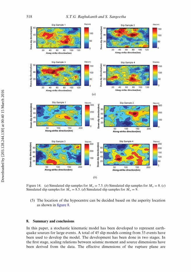
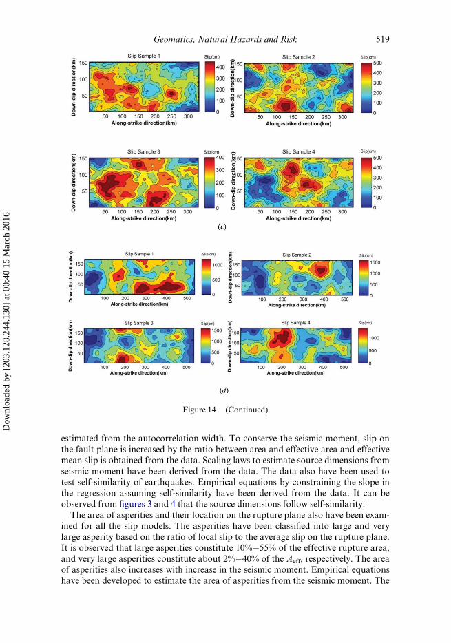
(4) Once the correlation lengths are fixed, simulate the standardized slip as a von
Karman random field from the spectral representation method of Shinozukaand Deodatis (1996) or Fourier integral method of Pardo-Igu´zquiza and
Chica-Olmo (1993). Generate the slip field from equation (4). An ensemble of
slip models can be simulated from this procedure. Figure 14(a)�(d) shows the
simulated slip samples forMw D 7.5, 8, 8.5, 9, respectively.
Table 7. Coefficients for the scaling of correlation lengths ax and az for the autocorrelationfunction with source parameters log10(Y) D C0 C C1 (X).
X C0 C1 s(e)
Along-strike (Y D ax)
Mw ¡1.1090 0.2903 0.4194
Leff 0.7699 0.0025 0.3649
Weff 0.9705 0.0026 0.4284
Down-dip (Y D az)
Mw ¡2.5736 0.4475 0.3700
Leff 0.5171 0.0027 0.3500
Weff 0.4945 0.0056 0.3226
Table 8. Estimates of length, width, correlation lengths(ax, az) and Hurst exponents,H, forslip models for varying magnitudes.
Mw
Slip parameters 7.5 8 8.5 9
Subfault size, dx (km) 1 1 1 1
Subfault size, dz (km) 1 1 1 1
L (km) 100 176 312 551
W (km) 47 83 146 258
A (1EC005 sq. km) 0.047 0.146 0.456 1.422
D (cm) 67 119 211 373
sD (cm) 72 128 226 399
Leff (km) 71 125 221 390
Weff (km) 35 61 108 191
Deff (cm) 35 61 108 191
ALA (1EC005 sq. km) 0.012 0.037 0.116 0.370
AVLA (1EC005 sq. km) 0.005 0.017 0.053 0.169
ACA (1EC005 sq. km) 0.017 0.055 0.176 0.560
RDmax (km) 16.94 29.96 52.97 93.65
RLA (km) 4.77 8.44 14.93 26.39
RVLA (km) 7.23 12.78 22.59 39.95
Correlation length, ax (km) 11.70 16.35 22.83 31.89
Correlation length, az (km) 6.06 10.15 16.99 28.44
Hurst exponent,H 1.19 1.33 1.49 1.67
Geomatics, Natural Hazards and Risk 517
Dow
nloa
ded
by [
203.
128.
244.
130]
at 0
0:40
15
Mar
ch 2
016
(5) The location of the hypocentre can be decided based on the asperity location
as shown in figure 8.
8. Summary and conclusions
In this paper, a stochastic kinematic model has been developed to represent earth-
quake sources for large events. A total of 45 slip models coming from 33 events have
been used to develop the model. The development has been done in two stages. In
the first stage, scaling relations between seismic moment and source dimensions have
been derived from the data. The effective dimensions of the rupture plane are
Figure 14. (a) Simulated slip samples forMw D 7.5. (b) Simulated slip samples forMw D 8. (c)Simulated slip samples forMw D 8.5. (d) Simulated slip samples forMw D 9.
518 S.T.G. Raghukanth and S. Sangeetha
Dow
nloa
ded
by [
203.
128.
244.
130]
at 0
0:40
15
Mar
ch 2
016
estimated from the autocorrelation width. To conserve the seismic moment, slip on
the fault plane is increased by the ratio between area and effective area and effective
mean slip is obtained from the data. Scaling laws to estimate source dimensions from
seismic moment have been derived from the data. The data also have been used totest self-similarity of earthquakes. Empirical equations by constraining the slope in
the regression assuming self-similarity have been derived from the data. It can be
observed from figures 3 and 4 that the source dimensions follow self-similarity.
The area of asperities and their location on the rupture plane also have been exam-
ined for all the slip models. The asperities have been classified into large and very
large asperity based on the ratio of local slip to the average slip on the rupture plane.
It is observed that large asperities constitute 10%�55% of the effective rupture area,
and very large asperities constitute about 2%�40% of the Aeff, respectively. The areaof asperities also increases with increase in the seismic moment. Empirical equations
have been developed to estimate the area of asperities from the seismic moment. The
Figure 14. (Continued)
Geomatics, Natural Hazards and Risk 519
Dow
nloa
ded
by [
203.
128.
244.
130]
at 0
0:40
15
Mar
ch 2
016
large asperities are consistent with self-similarity, whereas the size of very large asper-ities deviates from self-similarity.
The hypocentre location on the rupture plane does not show any pattern with
magnitude, whereas the location of asperities from hypocentre increases with
increase in the seismic moment. The closest distance to regions of maximum slip and
very large asperity is consistent with self-similarity. The normalized distance from
hypocentre to asperities indicates that hypocentres are located closer to asperities.
Modelling the slip distribution on the rupture plane as a random field also has
been explored in this paper. This helps to understand the interaction between the slipon the neighbouring subfaults. The two-dimensional PSD is estimated from the slip
model by Fourier transform. The correlation lengths are different in along-strike and
down-dip directions indicating that the slip field is anisotropic. Gaussian, exponen-
tial and von Karman PSD are fitted to the data by estimating the correlation lengths
along the length and width of the rupture plane. It is observed that von Karman
PSD models the spectral decay of the slip field better than Gaussian and exponential
models. The correlation lengths increase with increase in the magnitude of the event.
Empirical equations to estimate the parameters in the von Karman PSD from magni-tude are derived from the data.
The results presented in this paper will be of use to engineers in simulating ground
motion for large events. Given a particular fault and magnitude, the developed
model can handle uncertainties in the slip distribution. The seismic moment can be
estimated from the magnitude through empirical relations. The length, width and
mean slip can be estimated from equations (1) and (2) from the seismic moment.
Once the rupture dimensions are known, correlation lengths can be determined by
using equation (10) and coefficients reported in table 7 from the magnitude of theevent. Sample realizations of the standardized slip field can be simulated by the spec-
tral representation of Shinozuka and Deodatis (1996) by replacing sequences of ran-
dom phase angles. The hypocentre should be located closely to the location of large
asperity on the rupture plane. An ensemble of slip fields can be generated from this
procedure. There are several methods available in the literature to generate ground
motion time histories for a given slip model (Douglas & Aochi 2008; Raghukanth
2008). Several samples of ground motion time histories can be generated from this
procedure. The developed stochastic source model for large events will find applica-tions in simulating ground motion for scenario earthquakes in seismic hazard analy-
sis. The equations developed in this study have to be updated as more slip models
become available.
References
Aki K, Richards PG. 1980. Quantitative seismology: theory and methods. Vol. 1. New York
(NY): WH Freeman; p. 1�700.
Bird P. 2003. An updated digital model of plate boundaries. Geochem Geophys Geosyst.
4:1525�2027.
Bracewell RN. 1986. The Fourier transform and its applications. New York (NY): McGraw-
Hill.
Douglas J, Aochi H. 2008. A survey of techniques for predicting earthquake ground motions
for engineering purposes. Surv Geophys. 29:187�220.
Hanks TC, Kanamori H. 1979. A moment magnitude scale. J Geophys Res. 84(B5):2348�2350.
520 S.T.G. Raghukanth and S. Sangeetha
Dow
nloa
ded
by [
203.
128.
244.
130]
at 0
0:40
15
Mar
ch 2
016
Hartzell S, Harmsen S, Frankel A, Larsen S. 1999. Calculation of broadband time histories of
ground motion: comparison of methods and validation using strong ground motion
from the 1994 Northridge earthquake. Bull Seismol Soc Am. 89:1484�1506.
Hartzell S, Heaton T. 1983. Inversion of strong ground motion and teleseismic waveform data
for the fault rupture history of the 1979 Imperial Valley, California, earthquake. Bull
Seismol Soc Am. 73:1553�1583.
Hartzell S, Liu P. 1995. Determination of earthquake source parameters using a hybrid global
search algorithm. Bull Seismol Soc Am. 85:516�524.
Ji C, Wald DJ, Helmberger DV. 2002. Source description of the 1999 Hector mine, California,
earthquake, Part I: wavelet domain inversion theory and resolution analysis. Bull Seis-
mol Soc Am. 92(4):1192�1207.
Lavall�ee D, Liu P, Archuleta RJ. 2006. Stochastic model of heterogeneity in earthquake spatial
distributions. Geophys J Int. 165:622�640.
Mai PM, Beroza GC. 2000. Source scaling properties from finite-fault-rupture models. Bull
Seismol Soc Am. 90(3):604�615.
Mai PM, Beroza GC. 2002. A spatial random field model to characterize complexity in earth-
quake slip. J Geophys Res. 107:1�28.
Mai PM, Spudich P, Boatwright J. 2005. Hypocenter locations in finite-source rupture models.
Bull Seismol Soc Am. 95:965�980.
Pardo-Igu´zquiza E, Chica-Olmo M. 1993. The Fourier integral method: an efficient spectral
method for simulation of random fields. Math Geol. 25:177�217.
Raghukanth STG. 2008. Modeling and synthesis of strong ground motion. J Earth Syst Sci.
117:683�705.
Raghukanth STG. 2010. Intrinsic mode functions of earthquake slip distribution. Adv Adapt
Data Anal. 2(2):193�215
Raghukanth STG. 2011. Seismicity parameters for important urban agglomerations in India.
Bull Earthquake Eng. 9(5):1361�1386.
Raghukanth STG, Iyengar RN. 2008. Strong motion compatible source geometry. J Geophys
Res-Sol Ea. 113(B4):B04309. doi:10.1029/2006JB004278
Raghukanth STG, Iyengar RN. 2009. Engineering source model for strong ground motion.
Soil Dyn Earthq Eng. 29:483�503.
Shinozuka M, Deodatis G. 1996. Simulation of multi-dimensional Gaussian stochastic fields
by spectral representation. Appl Mech Rev. 49(1):29�53.
Somerville P, Irikura K, Graves R, Sawada S, Wald D, Abrahamson N, Iwasaki Y, Kagawa T,
Smith N, Kowada A. 1999. Characterizing crustal earthquake slip models for the pre-
diction of strong ground motion. Seismol Res Lett. 70(1):59�80.
Vanmarcke EH. 1983. Random fields: analysis and synthesis. Cambridge (MA): MIT Press.
Geomatics, Natural Hazards and Risk 521
Dow
nloa
ded
by [
203.
128.
244.
130]
at 0
0:40
15
Mar
ch 2
016
Recommended