Download pdf - A stochastic model for neuronal bursting

BioSystems 33 (1994) l-16

A stochastic model for neuronal bursting

Arnold0 Frigessi* a, Petr L6nskib, Angela B. Mariottoc*d

aLaboratorio di Statistica, Universitri di Vene:ia. Ca’ Foscari, Dorsoduro 3246, I-30123 Vene:ia, Italy

blnstitute o_f Physiology. Academy oj Sciences, Videriski 1083. 142 20 Praha 4-KrC: C:ech Republic

cistituto per le Applica:ioni de1 Calcolo ‘Mauro Picone’. CNR. Viale drl Policlinico 137, l-00161 Rome. Ital)

‘lstituto Superiore di Sanita: Laboratorio di Epidemiologia e Biostatistica, Viale Fegina Elena 299. I-00161 Ram;. Ita!v

Received 14 July 1993

Abstract

A new stochastic model for bursting of neuronal tiring is proposed. It is based on stochastic diffusion and related to the first passage time problem. However, the model is not of renewal type. Its form and parameters are physiologically interpretable. Parametric and non-parametric inferential issues are discussed.

Keywords: Neuronal model; Membrane potential; Bursting: Stochastic process; Statistical inference

1. Introduction

Stochastic diffusion neuronal models represent one of the most advanced and successful descriptions of the membrane electric potential of a neuron. Most of these models presented in the literature have a common property: they generate spike trains that are of renewal type and whose interspike intervals (ISIS) have a unimodal probability density function. In experiments with spontaneous or driven neuronal activity, cases are often encountered for which one or both of these conditions are not met. The main aim of this paper is to propose a very simple model, which is based on stochastic diffusion and is physiologically interpretable, that allows these drawbacks to be over-

* Corresponding author.

come. It describes the so called bursting activity of a neuron. The model is intended mainly for a neuron within a neural network; however, the wiring of the net is not specified.

Bursting is a very frequent type of neuronal behaviour. A broad class of quite different phenomena are classified as bursts. The common feature consists in a sequence of ‘short’ ISIS separated by one (or a few) ‘long’ interval(s). The next section of this paper tries to put some order in an ample and scattered literature on this topic. We survey and present some of the main models and their applications. Physiological objections are pointed out on the basis of selected experimental findings. General features of bursting are col- lected, in order to be incorporated in our new model. In Section 3 we define the model, in terms of stochastic diffusions and their first hitting times

0303-2647/94/$07.00 0 1994 Elsevier Science Ireland Ltd. All rights reserved SSDI 0303-2647(93)01429-W

2 A. Frigessi et al. / BioSvslems 33 (1994) l-16

to certain thresholds. Illustrative examples of the model simulation are presented. Although our model is certainly a very rough approximation of the true membrane dynamics, its form and all its parameters possess a physiological interpretation. For this reason not only the qualitative characteristics of our model are compared with experimental data, but also the inferential problems are considered. The mathematical model allows us to construct statistical parameter estimation pro- cedures as described in Section 4.

2. Bursting neuronal activity

Bursting pacemaker neurons have been often described in invertebrate animals. In these it has been proven that the burst arises from an endogenous pacemaker mechanism rather than from exter- nal synaptic input. This type of activity can be found, for example, in abdominal ganglia of slugs and snails, and in cardiac pacemaker cells or stomatogastic ganglion cells of crustacea. Katayama (1973) presented several other examples of this bursting activity with quantitative descriptions of the experimental results. Although our aim is to analyse a non-endogenous activity, which is not perfectly stereotyped as in the cases mentioned above, we will mention it here. The reason is, on the one hand, to stress the distinction from the stochastic bursting, and on the other hand, to point out features also applicable in our problem. There is greater experimental evidence about the bursts and their discharge patterns. Also, a very precise formulation of the terms which are in use for the mathematical models exists (Carpenter, 1981). Nevertheless, we mention this type of bursting not only because of the formal reason, but also because of the the possibility that the burst patterns in these neurons could be also under the control of some exogenous factors (see, for example, Pin and Gala, 1983).

Some common features in bursting patterns can be found. Often the length of the interburst interval depends on the number of spikes in the preceeding burst; the first IS1 within the burst tends to correlate with the interburst interval preceeding the burst. Clearly, the instant of spike generation need not be of renewal type. Also, the number of

spikes and the ISIS within the burst are variable. There are several spike pattern classifications. For the parabolic bursters the spiking frequency first increases and then decreases. For some others, the falling or the increasing phase is not necessarily present. The mathematical modelling of endogenous pacemaker bursting presented in the literature is based on the analysis of Hodgkin-Huxley type deterministic models (e.g., Plant, 1981). Here one may introduce an aperiodic discharge by means of the :heory of chaos (Chay and Rinzel, 1985) or by introducing noise into the *Hodgkin-Huxley system (Carpenter, 1981). Chay (1990) studied a deterministic model in which a voltage-activated Ca2+ channel inactivates slowly upon hyperpolarization. In her model, bursting is controlled by the relaxation time constant of the K+ channel that is activated by voltage. A sigmoidal shape (Boltzmann form) is assumed for the relaxation curve with respect to the voltage.

The spike trains recorded in the central nervous system of mammals sometimes have bimodal or multimodal IS1 histograms and exhibit bursting behaviour, for example the pyramidal cells of the hippocampus treated by penicillin, (Traub and Llinas, 1979), and the neurons of the mesencepha- lit reticular formation (Yamamoto and Nakahama, 1983; Yamamoto et al., 1986; Lansky and Radii, 1987). Bishop et al. ( 1964) presented experimental data of bursting character recorded in lateral ge- niculate neurons of anaesthetized cats. Legendy and Salcman (1985) studied in detail bursting phenomenon in neurons of the striate cortex of anaesthetized cats. They called burst an epoch of elevated discharge rate. For this purpose they defined, approximately, a burst as a minimum of three spikes for which the largest spacing was less than a half mean ISI (for precise definition see the cited paper). The size of burst is thus at least three for these authors. Abeles et al. (1990) investigated high-frequency bursts of activity recorded from the cortical areas. These authors also applied the term ‘burst’ in a highly restrictive sense and they concluded that the probability of observing a burst in one neuron was not affected by the fact that another adjacent neuron emmited a burst. Many other experimental data of this type have been col- lected.

A. Frigessi et al. / BioSystems 33 (1994) I - 16 3

Theoretical models for the bursting phenomena often based on the assumption that the neuron alternates between two states. The OFF state. during which no spike can be generated, and the ON state, when spikes are produced. Smith and Smith (1965) presented the classical model of this type producing a mixture of two exponentials as the ISI distribution. Thomas (1966) introduced a mode] for a bursting neuron based on the intraneuronal mechanism proposed by Burns (1955). The model is similar to a branching Poisson process and analogously to the model of Smith and Smith (1965) it can be formulated as a two-state semi- Markov process. Bursting in mesencephalic reticular formation neurons was recently studied by Griineis et al. (1989). A branching Poisson process (also called the Bartlett-Lewis process) is used in their description; the difference between their model and that of Thomas (1966) is that Thomas’s model does not permit overlapping of subsidiary processes. There, in the branching Poisson process, a series of primary events is assumed to form a stationary Poisson process. The secondary process consists of a random number of spikes and intervals that follow a gamma distribution. These assumptions permit the authors to compare the model with experimental data. For our model two of their conclusions are important. The first one is a Markov-dependency in the ISI structure, suggesting that the neuron output process holds memory about the input for a time which corresponds to the duration of burst. The second conclusion concerns the distribution of the intervals between spikes within a burst, which turns to be of gamma type, with a shape close to the inverse Gaussian distribution.

Ekholm (1972) modelled this type of neuronal activity as a generalized semi-Markov process, named pseudo-Markov process. In an extensive paper by de Kwaadsteniet (1982), the model proposed by Ekholm is called a semi-alternating renewal model and is analysed in more detail. Despite a close resemblance of the output of the model with the experimentally measured data, a serious objection must be raised: in the model formulation the number of spikes in the burst is determined a priori when the burst starts. This is physiologically hardly possible, because the num-

her of spikes in the burst is determined by the dynamics of the neuronal input during the whole bursting period.

The selective interaction models and the models with subthreshold interaction (for a survey see

Holden 1976; Lansky, 1983a) are also aimed at

describing bursting activity. The first of them seems to ignore relevant physiological properties by not taking into account any subthreshold inter- actions between excitation and inhibition, or more generally, any form of temporal facilitation. This defect is removed in the models with subthreshold interaction; however, there are also some objections in this case. Namely, no spontaneous decay is included ,in the membrane behaviour and the discretization of the membrane potential is too rough a simplification.

Kohn (1989) introduced a model neuron divided into two compartments: (I) the dendritic tree and the cell body, and (2) the trigger zone. Simulating this model he observed bursting activity. A sequence of action potentials was defined as a burst if at least six consecutive action potentials occured with corresponding interspike intervals less than the mean interval divided by 2.5. The bursting was always reflected by positively correlated interspike intervals and their variance was high with respect to the mean. Analogous results were predicted in Rospars .and Lansky .( 1993) for a model neuron with partial reset of the membrane potential. These two model neurons are endogenous bursters since the bursting does not arise due to the modu- lation of the input but due to the internal properties of the neurons.

Holden (1976) surveyed an alternative approach to bursting discharge patterns. It is based on a numerical and simulated investigation of two leaky neuronal integrators with mutual inhibitory coupling. The output of the model shows the multimodal histogram of ISIS, though the inputs are of temporally homogeneous Poisson type. Pairs of neurons,. reciprocally coupled by inhibitory synapses, also give rise to typical patterns of alternating bursts A see the study by Perkel and Malloney (1974). Zeevi and Bruckstein (198 I) and

Bruckstein and Zeevi (1985) analysed a genera] neural encoding model based on an ‘integrate-and- fire at threshold’ scheme. The main feature of their

4 A. Frigessi et af. / BioSys~ems 33 (1994) I-16

model is that it takes into account that the membrane integrates an effective ionic current, which depends not only on the input generator current but also on the output-dependent self-inhibition feedback. This type of feedback can be thought of as a source of systematic variability, which can be incorporated into the class of stochastic bursting model that we describe next.

Recently the rythmical synchronization of the neurons in the visual cortex was experimentally studied (Eckhom et al., 1988; Gray and Singer, 1989). It is hypothesized that lower-order neurons can produce an oscillation of activity in a phase as a response to specific inputs. The resulting postsynaptic potentials in the target cells produce a large oscillation in their membrane potential. At the peak of this oscillation, the membrane potential of the higher order neuron would fire a high- frequency burst of spikes (Styker, 1989). Theo- retically, it corresponds to the periodical input to a higher-order model neuron. It is well known that such periodical input can, for appropriately chosen parameters, produce high-frequency firing during its elevated level while it remains almost si- lent during the lower phase of the input (Gummer, 1991a,b; L6nsky et al., 1992). This is one of the alternative mechanisms to the inhibitory feedback which can be a source of bursting in a neural network. Both these cases are examples of input controlled bursting.

3. The model

3.1. General description The neuronal output may be considered as a

realization of a point process. This process is generated in most of the neuronal models by the first passages of a stochastic process, called membrane potential or generator potential, through a threshold potential, usually (but not always) deterministic. During bursting the underlying generator potential changes according to the state of the activity. The neuronal behaviour is epitomized by a time-continuous one-dimensional real valued stochastic process describing the membrane potential. Additionally, there are again two alternating states in which the neuron can be. These states are called ‘bursting’ and ‘inactive’ periods. We assume

that the parameters in the model can change only at the moment of spike generation but not during the ISI. This &mplification is reasonable and allows us to avoid unnecessary mathematical com- plications. Hence, the values of the parameters, which are reset at the beginning of the ISI, are to be considered as average values valid over the whole interval. The state of the neuron depends on the trajectory of the membrane potential from the moment of the !ast spike generation. An analogous mechanism was used by Frigessi and den Hollander (1989) for modeling a stimulated neuron.

Three constants are important for the neuron characterization. The first of them is a threshold potential A. Whenever the membrane potential reaches the value of the threshold potential A then an action potential (spike) is generated. Instan- tanously the value of the membrane potential is reset to the resetting potential B c A. The resetting potential B may simulate the role of spatial facilitation in neuronal firing (e.g. Schmidt, 1978). The resetting to the level different from the resting potential was studied by Lansky and Smith (1989) and Lansky and Musila (1991) but there the neuronal firing output was of renewal character. A di”- ferent interpretation of the resetting potential B may follow from consideration of the postinhibitory rebound. That phenomenon is a non-linear increase of the excitability of the neuron after a period of hyperpolarization (e.g., Perkel et al., 1981). The third constant R, identified as the resting potential, is the potential across the neuronal membrane, provided that no special stimuli act on the cell from outside. Falling to rest is due to a relatively long period without a response to the input signal. The character of the process describing the membrane potential changes at the moment when its trajectory reaches the resting potential R < A. The inactive state is precisely defined as an IS1 during which the level R is reached by the the membrane potential. So, it is com- posed of two parts: the first one is the time elapsed from the last action potential (when A was reached) to the crossing of level R. The second one is the time necessary to produce the new next action potential, i.e. the time to the next crossing of the threshold A starting from R.

A. Frigessi et al. / BioSystems 33 (1994) 1-16 5

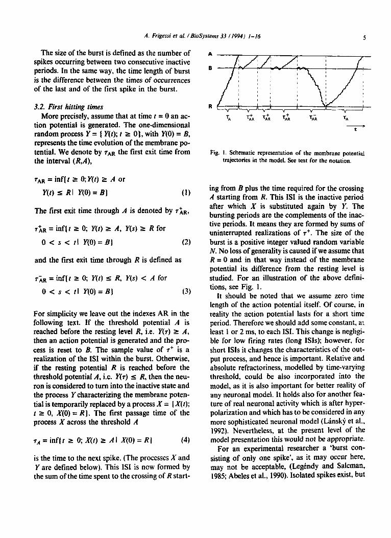
The size of the burst is defined as the number of spikes occurring between two consecutive inactive periods. In the same way, the time length of burst is the difference between the times of occurrences of the last and of the first spike in the burst.

3.2, First hitting times More precisely, assume that at time t = 0 an ac-

tion potential is generated. The one-dimensional random process Y = 1 Y(t); t 1 01, with Y(0) = B, represents the time evolution of the membrane potential. We denote by TAR the first exit time from the interval (&A),

TAR = inf( f k O;Y(r) L A or

Y(t) z RI Y(0) = B) (1)

The first exit time through A is denoted by r&+

& = inf( t 2 0; Y(r) L A, Y(s) 1 R for

0 < s < tl Y(O)=B) (2)

and the first exit time through R is defined as

riu = inflt 1 0; Y(t) 5 R, Y(s) < A for

0 < s < fl Y(O)=B] (3)

For simplicity we leave out the indexes AR in the following text. If the threshold potential A is reached before the resting level R, i.e. Y(r) L A, then an action potential is generated and the process is reset to B. The sample value of T+ is a realization of the IS1 within the burst. Otherwise, if the resting potential R is reached before the threshold potential A, ix. Y(T) I R, then the neuron is considered to turn into the inactive state and the process Y characterizing the membrane potential is temporarily replaced by a process X = [ A’( 1);

t 2 0, X(0) = R J. The first passage time of the process X across the threshold A

TA=inf(t L O;X(r)l Al X(O)=R) (4)

is the time to the next spike. (The processes X and Y are defined below), This IS1 is now formed by the sum of the time spent to the crossing of R start-

t -

Fig. I. Schematic representation of the membrane potential trajectories in the model. See text for the notation.

ing from B plus the time required for the crossing A starting from R. This IS1 is the inactive period after which X is substituted again by Y. The bursting periods are the complements of the inactive periods. It means they are formed by sums of uninterrupted realizations of T+. The size of the burst is a positive integer valued random variable N. No loss of generality is caused if we assume that R = 0 and in that way instead of the membrane potential its difference from the resting ievel is studied. For an illustration of the above definitions, see Fig. 1.

It should be noted that we assume zero time length of the action potential itself. Of course, in reality the action potential lasts for a short time period. Therefore we should add some constant, a: least 1 or 2 ms, to each ISI. This change is negligible for low firing rates (long ISIS); however, for short ISIS it changes the characteristics of the output process, and hence is important. Relative and absolute refractoriness, modelled by time-varying threshold, could be also incorporated into the model, as it is also important for better reality of any neuronal model. It holds also for another feature of real neuronal activity which is after hyperpolarization and which has to be considered in any more sophisticated neuronal model (Lansky et al., 1992). Nevertheless, at the present level of the model presentation this would not be appropriate.

For an experimental researcher a ‘burst con- sisting of only one spike’, as it may occur here, may not be acceptable, (Legendy and Salcman, 1985; Abeles et al., 1990). Isolated spikes exist, but

6 A. Frigessi et al. / BioSysretns 33 ( 1%hfJ I- 16

would not be considered bursts. Truly. their experimental data; Gummer ( 1991a) used the ran- character is different and from the experimental dom walk version as the starting point for his at- point of view they belong to the inactive period. tempts to model the effect of time-variable input The previous definitions could be easily refor- intensity and Berger and Pribram (1992) applied mulated so that an isolated spike would not inter- the model for the description of visual cortex neu- rupt the inactive period. Since such changes would rons. We can see that after three decades the mode1 cause some notational inconveniencies we will not still plays its role in the theoretical description of pursue them any further. neuronal tiring.

3.3, The membrane potential in the bursting and

inactive states

There exists a large choice for the model of membrane potential (Tuckwell, 1988) and generally an increase of their biological reality induces lower mathematical tractability. For this reason we start with one of the simplest possibility. Assume that the process Y within any given IS1 is a Wiener process

The parameters p and u appearing in the Wiener process have a physiological interpretation which follows from the diffusion approximation. Name- ly, it is

cr = ah - do, a2 = a% + d’w (6)

We assume below that the model is controlled only by the input intensities and that the PSP sizes are equal and constant. so that

dY(t) = bdt + udB’(t) (5) p = a(h - w), a* = a’(h + w) (7)

where p and u > 0 are constants ant’ W = ( W(t).

t 2 0) is a standard Wiener process. The process Y defined above represents a diffusion approximation of a model describing the membrane potential behaviour as a random walk (Gerstein and Mandelbrot. 1964). In that interpretation the excitatory postsynaptic potentials (EPSP) of size a > 0 and the inhibitory postsynaptic potentials (IPSP) of size d > 0 arrive in accordance to two independent Poisson processes with intensities h and o. Such inputs are summed on the membrane of the neuron. The basic requirements for the diffusion approximation to be valid are ‘small’ values of jumps a and d, and simultaneously ‘large’ values of input intensities h and w. Less heuristic and more detailed descriptions with generaliza- tions can be found in several papers on this topic, reviewed by Tuckwell (1988). Stevens (1964) argues in favor of model 5 in the following way: ‘It is well known that in intracellular records from several different types of repetitively discharging neurons, the membrane potential repolarizes at the end of each spike, and then increases approximately linearly to the firing level where the next spike is initiated. Superimposed upon this linearly increasing depolarization are haphazard membrane potential fluctuations’. Levine (1991. 1992) discussed in detail the fit of the model 5 with the

Let us summarize some properties concerning Y. The probability of reaching the threshold A before hitting R is

PA = Prob( Y(r) = A)

= 1 - wCW@ - RN 1 - exp(-2+(A - R)

(8)

where we denote 4 = $u’ (Karlin and Taylor, 1975). Eq. 8 gives the probability that the next spike will belong to the burst. It is important to determine under which conditions PA = I. This means that the bursting state of the neuron is per- sistent, with negligible probability of passing to the inactive period. If P*” = 0, then the burst is ending. The first term of the Taylor series expan- sion for small d, is

If C#J >> (B - R)-’ then PA = 1. For the relative input intensity defined as $ = h/o the condition is

II = B-R+a

B-R-a (10)

A. Frigessi et al. 1 BioSystems 33 (1994) 1-16 7

The probability distribution of the time to the next spike within a burst is crucial. Denote the cumulative distribution function for exits from ,4 by F+(t) = Prob(r+ < f) and the corresponding Laplace transform by p(s); analogously F-(t) is the cumulative distribution function for exits from R and!-(s) its Laplace transform. It is

sinh(J(B - B)) (1 I) sinh(J(A - R))

where J = Q-~~(B~ + 2g2s), and for the first two moments of the exit time we have

siderably when R - -00, for which, with one absorbing boundary, we have

- f?l - op (w,u) = 2s exp c (A - 9 - pt)2

- - 20% >

(14)

This is the inverse Gaussian distribution (IGD) and its properties are extensively surveyed by Chhikara and Folks (1989). For example if (A - B)b - 00 then the IGD converges to the

E(r+) = exp #(A - B) f 3

(A - B) sinh(W - R)) cosh(+(A - R)) - (B - R) cosh@(B - R)) sinh(4(A - R)

dsW44A - RN2

B(A2 - B2 + 2R(A - B)) z

3&A

as p becomes small. Further

E((rfJ2) = exp[#(A - B)> i

(8’ - A’ + 2R(A - B)) sinh(9(B - R)) __c_-~ 3

+ sinh(4(A - R)

L(7+) 2lA - R) coshMA - R)) r#l + - ’ ___----.

CI sinh(#(A - R)) >

(13)

where 6 = p/a’. These calculations are based on the results of Darling and Siegert (1953). From Eqs. I2 and I3 one can also get the variance of 7+.

Obviously the same formulas are available for the exit through R.

Eq. 1 I gives the Laplace transform of the exit time distribution through A in the presence of a second boundary R. It can be simplified con-

(12)

normal distribution. In practice, the condition (A - B)@ > 5 is reported to be sufficient in order to approximate the IGD by a normal distribution.

It is a substantial question how well one can approximate y(r+,a) by the corresponding IGD. Eq. I I can be rewritten in the form

j%;r,d = exp[@(A - B)] exp[- J(A - B)]

1 - exp(-2J(B - R))

1 - exp(-2J(A - R)) = _7+, - 0 (wd

I - exp(-2$(B - R)Jl + 2s/& )

1 - exp(-2@( A - R)mT (15)

where the first term in Eq. 15, 3: _ oD (s;e,o), is the Laplace transform of the density function (Eq. 14). The second term in Eq. 15, for s = 0 is equal to PA, given in (8). Let us denote this second term in Eq. 15 as PA(S) By taking derivatives

8 A. Frigessi et al. / BioSystems 33 (1994) l-16

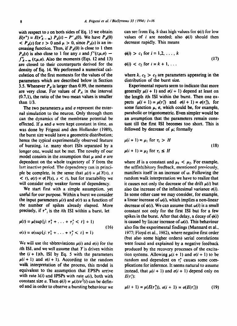
with respect to s on both sides of Eq. 15 we obtain E(r+) = E(r+A _ -) PA(s) - P’A(0). We have PA(O) < PA(s) for s > 0 and I( > 0, since PA(s) is an increasing function. Thus, if PA(O) is close to I then PA(s) is also close to 1 for any s and f’(t;p,u) - fi _ o (Q,u). Also the moments (Eqs. 12 and 13) are closed to their counterparts derived for the density of Eq. 14. We performed a numerical cal- culation of the first moments for the values of the parameters which are described below in Section 3.5. Whenever PA is larger than 0.99, the moments are very close. For values of PA in the interval (0.7,1), the ratio of the two mean values is smaller than l/3.

The two parameters p and u represent the exter- nal simulation to the neuron. Only through them can the dynamics of the membrane potential be effected. If ~1 and u were kept constant in time, as was done by Frigessi and den Hollander (1989), the burst size would have a geometric distribution; hence the typical experimentally observed feature of bursting, i.e. many short ISIS separated by a longer one, would not be met. The novelty of our model consists in the assumption that p and u are dependent on the whole trajectory of Y from the last inactive period. The dependency can in princi- ple be complete, in the sense that ~(1) = p( Y(s), s < t), u(f) = u( Y(s), s < I), but for tractability we will consider only weaker forms of dependency.

We start first with a simple assumption, yet useful for our purpose. Within a burst we consider the input parameters ~0) and u(t) as a function of the number of spikes already elapsed. More precisely, if r+i is the ith ISI within a burst, let

(16) u(f)=u(suplj:T~+...+rf< 1)+1)

We will use the abbreviations ~(0 and a(i) for the ith ISI, and we ~111 assume that Y is driven within the (i + l)th, ISI by Eq. 5 with the parameters cr(i + 1) and u((i + 1). According to the random walk interpretation of the process, this model is equivalent to the assumption that EPSPs arrive with rate h(i) and IPSPs with rate w(i), both with constant size a. Then 4(i) = p(i)/&(i) can be &fin- ed and in order to observe a bursting behaviour we

can see from Eq. 8 that high values for $(i) for low values of i are needed; also $(i) should then decrease rapidly. This means

$(i) > cl for i = 1,2, . . . , k

9(i) < c2 for i = k + 1, . . . (17)

where k, c2 > c2 are parameters appearing in the distribution of the burst size.

Experimental reports seem to indicate that more generally p(i + 1) and o(i + 1) depend at least on the length ith ISI within the burst. Then one ex- pects p(i+ 1) = ~(73 and u(i+ I) = ~~(72, for some function ~1, u, which could be, for example, parabolic or trigonometric. Even simpler would be an assumption that the parameters remain constant till the first ISI becomes too short. This is followed by decrease of p; formally

/&(i+ l)=p~ for ri > H

p(i+ l)=pz for ri I H (18)

where H is a constant and ~1 c pz. For example, the sellinhibitory feedback, mentioned previously, manifests itself in an increase of w. Following the random walk interpretation we have to realize that it causes not only the decrease of the drift p(i) but also the increase of the infinitesimal variance u(i). In some other case we may consider, for example, a linear increase of o(i), which implies a non-linear decrease of 4(i). We can assume that w(i) is a small constant not only for the first IS1 but for a few spikes in the burst. After that delay, a decay of b(i) is caused by linear increase of w(i). This behaviour also fits the experimental findings (Mannard et al., 1977; Floyd et al., 1982), where negative first order (but also some higher orders) serial correlations were found and explained by a negative feedback produced by the recovery processes of the excitation systems. Allowing p(I’. + 1) and u(i + 1) te be random and dependent on 7: causes some com- plications for inference. It seems natural to assume instead, that ~(i + 1) and u(i + 1) depend only on E(+:

p(i + 1) = p(E(Q), u(i + 1) = a(&;)) (19)

A. Frigessi et aI. / BioS_wetns 33 11994) 1-16 9

AS shown below, in this case one can perform estimation easily. Note also that the inferential problem here is non-parametric, since functions have to be estimated.

Most appropriate characterization following from our assumptions would be a dependency of ~(i + 1) and u(i + 1) on the entire burst, p(i + 1) = pL(rt, - - * , rf)andu(i+l)=u(rf,...,rt).Asan example we can consider a sigmoid function

p(i+ U=PO 1

1 + exp(@(rt + . . . + 7; - C))

(20)

where C is a constant controling the burst duration and 6 > 0 is a constant on which depends how sharp is the end of the burst. In inhibitory feedback interpretation the constant C reflects the delay after which the inhibition starts to affect the input of the neuron; then fl expresses the speed of the feedback reaction. We can also interpret Eq. 20 via the random walk model. As p is linear function of w, to get this shape for p the shape of w is mirror-like at C, however, this would also cause an increase of u. The form of the net excitation rate (Eq. 20) as it is implemented in the presented model can produce qualitatively similar tiring patterns as for periodically driven ~1 in a standard integrate-to-fire schema aimed on oscillation modeling (Gummer, 199lb; Lansky et al., 1992). The only substantial difference is that for Eq. 20, with suitable chosen parameters, the silence periods need not to be regular as it is in the case of periodical cc.

For a complete characterization of our model we must also define the process X. One can easily assume that crossing the level R, the membrane potential changes its character and starts to behave in a manner similar to a non-bursting neuron. Such neuron can be described by a general diffusion process (Lrlnsky and Lanska. 1987). All the available results on these processes can be used realizing that a burst can be viewed as a single event. In our exposition here, we avoid the com- plications of introducing this new process. We want to think X as being again a Wiener process as defined by Eq. 5 but with a drift L(X and in-

finitesimal variance u.~ that neither depends on Y, nor on the number of spikes in the preceding burst. Under this assumption a moment when the level R is reached is a regenerative time-point for the underlying model. Thus the burst lengths will form a renewal process. To introduce into the model some type of dependency of the bursting behaviour on the previous period of silence would be only a formal step. We do not include this just to make the model as transparent as possible.

3.4. The structure of the birrsr The probability p,, of the burst being of size II is

I, - I

P,, =Prob(N=n)=(l - P,:‘) n P4 (21) i= I

where the subscript i denotes the use of parameters r(i) and u(i) in the corresponding generation process, and PAi is given by Eq. 8. If G(i) were constant equal to 4, then, as mentioned before, Eq. 19 becomes a geometric distribution with E(N) =

(1 - PA)-’ and vur(ZV’) = PA(l - PA)-2. In the general case no analytical formulas for the moments of N are available. We can compute the distribution of the length of bursting period from the distribution of the individual IS1 lengths and from the distribution of the burst size; its Laplace transform is

00 n

3+(s) = C pn n3+ (w(ih4i)ln) (22) n= I i=l

where p’(s;p(i),u(i) In) denotes the conditional Laplace transform and pn is given by Eq. 19.

3.5. Model simulation and the physiological parameters

In this section we try to relate our model and its parameters more precisely to physiological studies. First, we fix, at least tentatively, the values of the parameters A, B and R. The value of the firing threshold is often reported to be close to -50 mV (-60 mV) and similarly the resting level R is accepted to be equal to -80 mV (- 90mV) (e.g. Schmidt, 1978) Thus we can assign as the reseting

IO A. Frigessi er al. / BioSptenrs 33 I19931 l-16

level the value B = -60 mV (-70 mV), After the (Tuckwell and Richter. 1978). Although the inten- transformation of R to 0. we have A E [20.40] and sities are not constant in our model, these values B c [10.40]. should be considered as guidelines.

Three parameters are left: the sizes of PSP u and the input intensities A and o. While for the size of the PSPs some information can be found in the experimental literature. the values of the input intensities are more or less only speculative. Usually the sizes of PSPs are considered to be identical constants. The range from 0.1 to 0.5 mV seems appropriate, and for them the diffusion ap proximation is likely to hold. These low values of PSP are interpreted in the following way: there are many synapses ending on the dendrites and thus the average change of the membrane potential due to a single PSP is not large. For the synapses at the soma the size of the PSP ranges from I mV to 3 mV. (Schmidt, 1978; Tuckwell. 1979). Musila and Lzinskj (1992a) studied variable synaptic input effect in a model neuron. Tuckwell (1979) used the excitatory intensity A = 1379 s-’ and the inhibitory intensity o = x/2. In many of his other papers the excitatory intensity ranges from hun- dreds to thousands per second and the inhibitory intensity is always lower or equal. This also corresponds to the estimated number of synapses

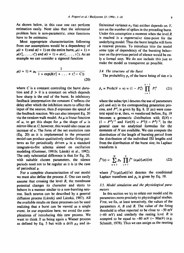
For the performance of the model the values of $ and $ are important. From Eq. 7 we deduce that if the inhibitory intensity o is negligible when compared with X. the excitatory one, then (I c I implies C#J > I. With increasing o the value of u has to decrease to achieve C#J > I. The parameter of relative input intensity J, is easier to interpret and Inequality IO ensures P.’ = I. For the numerical example suggested above a simple variant of Ine- quality IO. also giving PA very close to I, is $ >> (B - R + 3a)l(B - R - 3~). Taking B - R = 30 then, for a = 2. we obtain $ > 1.50; a = I, I/, > 1.22; and LI = 0.5. $ > 1.10. For small n, if the intensity of excitation is 10% higher than the intensity of inhibition, P” = 0.997. In Fig. 2 the dependency of PA on JI is illustrated. A numerical comparison of the moments in Eqs. I2 and I3 with their IGD equivalents shows no significant dis- crepancy if PA = I.

The quantitative description of experimental data on burst activity is very heterogenous. Smith and Smith ( 1965) fitted a mixture of two exponentials to data, thus also implying exponentially dis-

P”

l.O- /

mc.-._;.‘.“’ ..“, /-

. ..* ..*;

0.8- / *.*’ ’ . :‘/

Ii i 1:.

0.6- / ‘1

/ / jy

0.4 - / ::,/

/ / j,

0.2 - / : ; , .:*

/ . 2.. / / . ..* .

cd . ..a* 0 0 -v ’

__....a. -’ I -1 I I I I I I I I I I

0.2 0.4 0.6 0.8 I,0 1.2 1.4 1.6 q

Fig. 2. Dependency of upcrossing probabilities PA on relative input intensity $ = xiw for B - X = 30. A - R = 40. Different lines indicate the value of PSP: - - - for a = 2. - - - for a = I: and -_- for a = 0.5.

A. Frigessi et al. /BioSystems 33 (1994) 1-16 II

tributed ISIS within the bursts. Another example is by de Kwaadsteniet (1982). A case of very regular bursts is presented by Yamashita et al. (1983). Citing from it: ‘the mean burst cycle [the time from the beginning of one burst to the beginning of the next] was 19.9 * 4.2 s, burst duration was 6.5 f 1.7 s, and intraburst spike frequency was 6.6 f 1.1 Hz (S.E.)‘. Plnfortunately the possibility of comparing data from literature is thwarted by the different meanings given to the term ‘burst’.

For preliminary illustration we simulated the introduced model using the method described by Musila and Lansky (1992b) and in Lr-inskg and Lanska (1994). The simulation step used was 0.1. For simplicity we assumed that the infinitesimal variance was constant, mainly to make the simulation simpler and the results more transparent. The results of two simulation runs, each of the size 1000 ISIS, are presented.

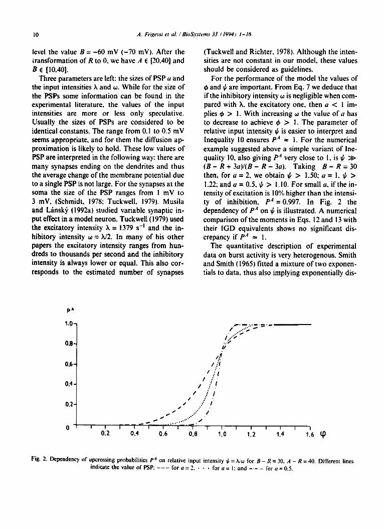
Example I. The schema of Inequalities 18 was applied with parameters A = 40, B = 30, a2 = 1, /.&I = 1, pz = - 1, H = 7. The mean and median ISI were 17.7 and 10.2, respectively (the unit of time is not specified on purpose as it corresponds to the units for cc. cr and H. and thus can be appropriately modified). The difference between these two characteristics of positions suggests that the distribution is not symetrical, which is apparent from the histogram (Fig. 3a). The histogram is bimodal and when compared with experimentally obtained ones it may seem too simple. Of course this ‘defect’

can be easily removed by increasing u or by decreasing the difference between pI and p2. The serial correlation coefficients were computed from the simulated data and are pictured in Fig. 3b. There is significantly negative first order serial correlation coefficient while those for all higher orders are close to zero. This feature is often observed experimentally on recorded spike trains having non-renewal character (for review see Linsky and Radil, 1987). No periodicity is apparent in this correlogram as well as in the computed periodogram. The coefficient of variation (CV = standard deviation/average) is a measure often used to characterize experimentally recorded ISIS (LBnsk$ and Radil, 1987) and for this example it equals 1.14.

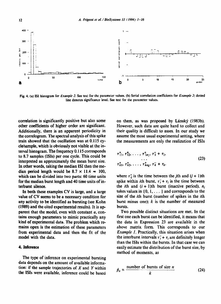
Example 2. For the second simulation we employed the schema of Eq. 20 with the parameters A = 20, B = 10, (Y’ = 1, h = 1 C = 60, /3 = 1.

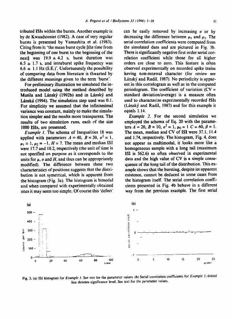
The mean, median and CV of IS1 were 37.1, 11.4 and 1.74, respectively. The histogram, Fig. 4, does not appear as multimodal, it looks more like a homogeneous sample with a long tail (maximum IS1 is 562.6) so often observed in experimental data and the high value of CV is a simple conse- quence of the long tail of the distribution. This example shows that the bursting, despite its apparent existence, cannot be deduced in some cases from the histogram itself. The serial correlation coefficients presented in Fig. 4b behave in a different way from the previous example. The first serial

(a) (b)

500 - -

l-

400 - !

c_ 300 - j -y P

kl I !

0 200 - j I [ Y) : : ; j : 3 2 loo- : ' 1

i? I i j

o- '- _---T--Y-_

0 20 40 60 80 100 rime

=

!

: : 0 -0 - -- -- -

- -- - _-- 0 "

7 i - ::

-1

0 5 10 15 20 25

order

Fig. 3. (a) ISI histogram for Exampie I. See text for the parameter values. (b) Serial correlation coefficients for Esomple I: dotted line denotes significance level. See text for the parameter values.

12 A. Frigessi et al. / BioSystems 33 (1994) I-16

d' 0 5 10 15 20 2: order

Fig. 4. (a) ISI histogram for Example 2. See text for the parameter values. (b) Serial correlation coefficients for Example 2; dotted line denotes significance level. See text for the parameter values.

correlation is significantly positive but also some other coefficients of higher order are significant. Additionally, there is an apparent periodicity in the correlogram. The spectral analysis of this spike train showed that the oscillation was at 0.115 cycle/sample, which is obviously not visible at the interval histogram. The frequency 0.115 corresponds to 8.7 samples (ISIS) per one cycle. This could be interpreted as approximately the mean burst size. In other words, taking the median IS1 then the median period length would be 8.7 x 11.4 = 100, which can be divided into two parts: 60 time units for the median burst length and 40 time units of interburst silence.

In both these examples CV is large, and a large value of CV seems to be a necessary condition for any activity to be identified as bursting (see Kohn (1989) and the cited experimental results). It is apparent that the model, even with constant u, con- tains enough parameters to mimic practically any kind of experimental data. The problem which remains open is the estimation of these parameters from experimental data and then the fit of the model with the data.

4. Inference

The type of inference on experimental bursting data depends on the amount of available information: if the sample trajectories of X and Y within the ISIS were available, inference could be based

on them, as was proposed by Lanskj, (1983b). However, such data are quite hard to collect and their quality is difficult to asses. In our study we assume the most usual experimental setting, where the measurements are only the realization of ISIS

where 7f is the time between the jth and 0’ + I)th spike within ith burst, 7T+ 7i is the time between the ith and (i + 1)th burst (inactive period), Hi takes values in (0, 1, . . . ) and corresponds to the size of the ith burst (number of spikes in the ith burst minus one); k is the number of measured bursts.

Two possible distinct situations are met. In the first one each burst can be identified, it means that the data in Expression 23 are available in the above matrix form. This corresponds to our Example I. Practically, this situation arises when the interburst intervals of+ 7i are definitely longer than the ISIS within the bursts. In that case we can easily estimate the distribution of the burst size, by method of moments, as

a, = number of bursts of size n

k (24)

A. Frigessi et al. / Bidystems 33 (1994) I-16 13

Then, inference on the parameters p(i) and o(i) must be based on the sample {r$, r+zi, . . . ,

7’kiif the columns in Expression 23, where the sample size ki is less than or equal to k, as some values may be missing, due to the fact that not all the bursts are of the same size. This means that the quality of the estimates for different cc(i) and u(i) will vary, typically decreasing in i. Also, some information is not exploited, as the inactive period is not used in the above described scheme. For experimental purposes, the estimation of p(i) and u(i) for small values of i may be sufficient.

Inference on the parameters of an IGD, given k independent realisations from it, can be performed by maximum likelihood or method of moments - see Chhikara and Folks (1989) for a complete treatment of this parametric case. We mentioned above that we may want to consider the case of Eq. 19 and p and u are to be estimated. For this purpose construct the set of points

(25)

where k* denotes the number of bursts of size j or bigger and fi(j + 1) is obtained using the above mentioned methods. The problem is now very classical: estimate a non-linear curve from the data point in Expression 25. The statistical literature is obviously extensive on this topic and software is amply available.

The second situation corresponds to our Exum- pie 2 and is entirely different. In reality, the data in Expression 23 are recorded in continuous time, from 71, to r/, + rk as n] + n2 + . . . + nk = hf

time intervals. A table like that in Expression 23 can be prepared, as we said above, if the bursts are well separated. Although this often happens, sometimes the bursts cannot be recognised. In this case the inference is much more difficult. Here is an outline of the problem. Let Tt, T2, . . . , TM be recorded ISIS. This sequence is highly correlated: q may be distributed in accordance with Eq. 11 with parameters p ( Tj _ I] and a( Tj _ 1) if it COT-

responds to an ISI within a burst; or 7-j may cor- respond to an inactive period, in which case it would be the sum of a random variable following Eq. 11 with parameters p [ Ti _ 11 and a( Ti _ I )

plus the hitting time of the process X, i.e. an IGD. If we assume that the hitting times are all distributed according to an IGD. we have essentially

+ (1 - qj) IGWP~ q- I )vul q -I IJW

+ IGWwwAR) 3 (26)

where 0 I ‘li 5 1. Estimation of the parameters for such a mixture model is a difficult task if no ad- ditional information is available (Amoh, 1984; Lbnsky and Smith, 1989). The latter paper pre- sents the results for IGD and its mixtures for the diffusion neuronal input integration with random initial depolarization. Fortunately, the model considered here can be simplified, in the following way. Since the bursts are not distinguishable, we may consider the parameters &I) and u(i) constant and equal to py and ur. In this case Tl, T2, . . . , TM are independent and identically distributed random variables with

Ti - rlIGD(lr Y,Q YAB)

+ (1 - dIGDtpx,ux,B,R) (27)

neglecting the last part of the silence period. i.e. transition from R to A (see Fig. 1). One has to estimate cy, uy, px, ux and the mixing parameter q. Clearly, also the thresholds A, B and R could be considered unknown at this point. Method of moments, maximum likelihood, minimum x2 and Bayesian methods have been all proposed for point estimation in mixture models (Titerington et al., 1985). A very succesful method for maximum likelihood estimation is the so called EM algorithm (Dempster et al., 1975), which we describe adapted to our problem. We first stan- dardize the 1GDs involved in our mixture: fi(t) corresponds to the process Y, fi(r) to the process X and they are

(28)

A. Frigessi’ et 01. / &System 33 (1994) I- 16 14

The log-likelihood function is

A-B 4 =---

PY ’ m2

The log-likelihood

A =-

PX

function is

M - 1 log(27r) - f

i = I i = I

i log Ti + i log Qi (29)

where Qi = 7)gi.t + (I - q)gi,2 and gij = J($) exp I -?,j Ti - m$2/(2mj2 Ti)), j = 1, 2. Taking the derivative of the log-likelihood function with respect to the 5 parameters and after some simplification we obtain, respectively, for 9, ml, m2, hl, and X2:

M

c gi.1 - gi.2

i=l Qi =*

M c _ ( Ti - jni)gi,,i =0, j=1,2

i= I Qi

(30)

(31)

1 --

( Ti - ntj)’

>

gij

Ai n+ Ti ---0, j=l,2 Qi

(32)

This system has to be solved. One way to solve it iteratively is by the EM algorithm. Given qfk),

mIk), m4 , k, hik), and X(ik)) the new values are obtained as

9 (33)

mfk+')= (i, TiHri,j)/i, it1i.j j= 1J (34)

j= 1,2 (35)

where we abbreviated Wi.1 = gi*t/Qi and w~i.2 = 1

- wil, computed using the values of the parameters at step k: qtk’, ml”), mjk), Xik', Xi"'. This iterative algorithm is known to converge to a local maximum of the likelihood function. Therefore a careful choice of the initial values q(O), mf*), mj*j, A/*), >rj*' is important. A reasonable guess for q(O) is generally not too difficult. We suggest 1 - q(O) = (expected size of burst)-‘. The other parameters should be initialized within their physiological ranges given in Section 3.5.

References

Abeles. A.. Vaadia. E. and Bergman, H.. 1990. Firing patterns of single units in the prefrontal cortex and neural network models. Network I. 13-25.

Amoh. R.K.. 1984. Estimation of parameters in mixtures of inverse Gaussian distributions. Commun. Stat. Part A Theor. Methods 13, 1031-1043.

Berger. D.H. and Pribram, K.H.. 1992. The relationship between the Gabor elementary function and a stochastic model of the inter-spike interval distribution in the response of visual cortex neurons. Biol. Cybern. 67, 191-194.

Bishop, P.O.. Lewick. W.R. and Williams. W.O.. 1964. Statistical analysis of the dark discharge of lateral genicu- late neurons. J. Physiol. 170. 598-612.

Bruckstein. A.M. and Zeevi Y.Y.. 1985. An adaptive stochastic mode) for the neural coding process. IEEE Trans. Syst. Man Cybern. 15. 343-351.

Burns. D.D.. 1955. The mechanism of afterbursts in cerebral cortex. J. Physiol. 127, 168-188.

Carpenter, G.A.. 1981. Signal patterns in nerve cells, in: Mathematical Psychology and Psychophysiology, S. Grossberg ted,) (SIAM-AM& Providence).

Chay. T.R.. 1990. Bursting excitable cell models by a slow Ca’+ current. J. Theor. Biol. 142. 305-315.

Chay, T.R. and Rinzel. J., 1985. Bursting. beating, and chaos in an excitable membrane model. Biophys. J. 47. 357-366.

Chhikara. R.S. and Folks, J.L.. 1989. The Inverse Gaussian Distribution (Marcel Dekker. New York).

Darling, P.A. and Siegert, A.J.F.. 1953. The first passage problem for a continuous Markov process. Ann. Math. Stat. 24, 624-639.

de Kwaadsteniet. J.W., 1982. Statistical analysis and stochastic modeling of neuronal spike train activity. Math. Biosci. 60. 17-71.

A. Frigessi et al. / BioSystems 33 (1994) 1-16 15

Dempster. A.P.. Laird. N.M. and Rubin. D.B.. 1977. Maxi- mum likelihood estimation from incomplete data via the EM algorithm. J. R. Stat. Sot B. 39. l-38.

Ekhorm. A., 1972. A generalization of the two-state two- interval semi-Markov model, in: Stochastic Point Processes, P.A.W. Lewis (ed.) (Wiley, New York).

Eckhom, R., Bauer. R., Jordan, W., Brosch, M., Kruse. W., Munk, M. and Reitboeck. H.J.. 1988. Coherent oscillations: a mechanism of feature linking in the visual cortex. Biol. Cybem. 60, 121-130.

Floyd, K.. Hick, V.E.. Holden. A.V.. Koley. J. and Morrison, J.F.B., 1982. Non-Markov negative correlation between interspike intervals in mammalian sympathetic efferent discharges. Biol. Cybern. 45. 89-93.

Frigessi. A. and den Hollander. F.. 1989. A stochastic model for the membrane potential of a stimulated neuron. J. Math. Biol. 27. 681-692.

Gerstein. G.L. and Mandelbrot. B.. 1964. Random walk models for the spike activity of a single neuron. Biophys. J. 5. 41-68.

Gray C.M. and Singer. W.. 1989, Stimulus-specilic neuronal oscillations in orientation columns of cat visual cortex. Proc. Natl. Acad. Sci. USA 86. 1698-1702.

Griineis. F.. Nakao. M.. Yamamoto. M.. Musha. T. and Nakahama. H.. 1989. An interpretation of Il’fluctuations in neuronal spike trains during dream sleep. Biol. Cybern. 60. 161-169.

Gummer. A.W.. 199la. Postsynaptic inhibition can explain the concentration of short inter-spike intervals in avian audi- tory nerve libres. Hearing Res. 55. 231-243.

Gummer, A.W.. 199lb. Probability density function of suc- cessive intervals of a nonhomogeneous Poisson process under low-frequency conditions. Biol. Cybern. 65. 23-30.

Holden. A.V.. 1976, Models of the Stochastic Activity of Neurones (Springer-Verlag. Berlin).

Karlin S. and Taylor H.. 1975. A First Course in Stochastic Processes (Academic Press, New York) p. 361.

Katayama. Y.. 1973. Electrophysiological identification of neurones and neural networks in the perioesophageal ganglion complex of the marine pulmonate mollusc. Onclddium verruculatum. J. Exp. Biol. 59. 739-751.

Kohn. A.F.. 1989. Dendritic transformations on random synaptic inputs as measured from a neuron’s spike train - modeling and simulation. IEEE Trans. Biomed. Eng. 36. 44-54.

Lgnskj, P., 1983a. Selective interaction models of evoked neuronal activity. J. Theor. Neurobiol. 2, 173-183.

Lgnskj, P., 1983b, Inference for diffusion models of neuronal activty. Math. Biosci. 67, 247-260.

Lbnsk$ P. and Lainski, V., 1987, Diffusion approximations of the neuronal model with synaptic reversal potentials. Biol. Cybern. 56. 19-26.

Lgnskj P. and LzinskB, V., 1994, First-passage-time problem for simulated stochastic diffusion processes. Comput. Biol. Med. 24, 91-101.

L&xl@, p. and Musila, M., 1991, Variable initial depolarization in the Stein’s neuronal model with synaptic reversal

potentials. Biol. Cybern. 64, 285-291.

LBnsk$ P. and Radil, T., 1987, Statistical inference on spontaneous neuronal discharge patterns. Biol. Cybern. 55, 299-3 I I.

LainskA P. and Smith, C.E., 1989, The effect of a random initial Value in neWal first-passage-time models, Math. Biosci. 93, 215-1917.

Lsinsk$ P.. Musila, M. and Smith, C.E., l992a, Effects of afterhyperpolarization on neuronal tiring. BioSystems 27, 25-38.

Lbnski, P., Rospars, J.-P. and Vaillant, J., l992b. Some neuronal modek with oscillatory input, in: Cybernetics and Sys- tems ‘92, R. Trappl (ed.) (World Scientilic Press, Singapore).

Legindy, C.R. and Salcman, M., 1985. Bursts and recurrences of bursts in the spike trains’ of spontaneously active striate cortex neurons. J. Neurophysiol. 53, 926-939.

Levine, M.W., 1991, The distribution of the intervals between neural impulses in the maintained discharges of retinal ganglion cells. Biol. Cybem. 65, 459-467.

Levine, M.W.. 1992, Modeling the variability of the firing rate of retinal ganglion cells. Math. Biosci. 112, 225-242.

Mannard, A., Rajchgot. P. and Polosa, C., 1977, Effect of post- impulse depression on background firing of sympathetic preganglionic neurons. Brain Res. 126, 243-26 I.

Musila. M. and Ltinskf, P., 1992a. A neuronal model with variable synaptic input effect. Cybern. Syst. 23, 29-40.

Musila. M. and Lrinskq, P.. l992b. Simulation of a dilTusion process with randomly distributed jumps in neuronal con- text. Int. J. Biomed. Comput. 31, 233-245.

Perkel, D.H. and Mulloney. B., 1974. Motor pattern produc- tion in reciprocally inhibitory neurons exhibiting postinhibitory rebound. Science 185, 181-183.

Perkel, D.H., Mulloney, B. and Budelli, R.W., 1981. Quantita- tive methods for predicting neuronal behavior. Neuros- cience 6, 823-837.

Pin, T. and Gola, M., 1983, Two identified interneurons modulate the tiring pattern of pacemaker bursting cells in Helix. Neurosci. L&t. 37, 117-122.

Plant, R.E., 1981, Bifurcation and resonance in a model for bursting nerve cells. J. Math. Biol. I I. 15-32.

Ricciardi, L.M., 1977, Diffusion Processes and Related Topics in Biology (Springer-Verlag. Berlin).

Rospars. J.-P. and Lsinskg, P.. 1993, Stochastic model neuron without resetting of dendritic potential. Application to first- and second-order neurons in olfactory system. Biol. Cybern. (in press).

Schmidt, R.F., 1978, Fundamentals of Neurophysiology (Springer-Verlag, Berlin).

Smith, D.R. and Smith, G.K., 1965. A statistical analysis of the continual activity of single cortical neurones in the cat unanaesthetized isolated forebrain. Biophys. J. 5-47-74.

Stevens, F.C., 1964. Letter to Editor. Biophys. J. 4. 417-419. Stryker, M.P., 1989, Is grandmother an oscillation? Nature 338.

297-298. Titterington, D.M., Smith, A.F.M. and Makov. U.E., 1985.

Statistical Analysis of Finite Mixture Distributions (Wiley,

New York). Thomas, E.A.C., 1966, Mathematical models for the clustered

16 A. Frigessi et al. ! BioSysrems 33 (1994) l-16

firing of single cortical neurones. Br. J. Math. Stat. Psycho) 19. 151-162.

Traub. R.D. and Llinas, R.. 1979. Hippocampal pyramidal cells: significance of dendritic ionic. J. Neurophysiol. 42. 476-496.

Tuckwell. H.C.. 1979. Synaptic transmission in a model for stochastic neural activity. J. Theor. Biol. 77, 65-81.

Tuckwell. H.C.. 1988. Introduction to Theoretical Neuro- biology (Cambridge University Press, Cambridge).

Tuckwell. H.C. and Richter, W., 1978. Neuronal interspike time distributions and the estimation of neurophysiological and neuroanatomical parameters. J. Theor. Biol. 71. 167-180.

Yamamoto. M. and Nakahama. H., 1983. Stochastic properties of spontaneous unit discharges in somatosensory cortex and mesencephalic reticular formation during sleepwaking states. J. Neurophys. 49. 1182-l 198.

Yamamoto, M., Nakaharna. H.. Shima. K.. Kodama, T. and Mushiake. H.. 1’386, Markov-dependency and spectral analysis on spike-counts in mesencephalic reticular neurons during sleep and attentive states. Brain Res. 366. 279-298.

Yamashita, H.. Inenaga, K., Kawata. M. and Sano. Y., 1983, Phasically firing neurons in the supraoptic nucleus of the rat hypothalamus: immunocytochemical and electrophysiological studies. Neurosci. Lett. 37. 87-92.

Zeevi. Y.Y. and Bruckstein. A.M., 1981, Adaptive neural en- coder model with selfinhibition and threshold control. Biol. Cybem. 40. 79-92.