Download pdf - A stochastic model for solidification

PRAMANA __ journal of

physics

© Printed in India Vol. 47, No. 6, December 1996 pp. 447-470

A stochastic model for solidification I. The basic equations, their analysis and solution

S H O B H A DASS, G A U T A M JOHRI* and L A K S H M A N PANDEY* Govt. M.H. College of Science and Home Science, Jabalpur 482 002, India *Department of Post Graduate Studies and Research in Physics, Rani Durgavati University, Jabalpur 482 001, India

MS received 4 April 1995; revised 8 November 1995

Abstract. A 3-dimensional (2-space, 1-time) model relating the diffusion of heat and mass to the kinetic processes at the solid-liquid interface, using a stochastic approach is presented in this paper. This paper is divided in two parts. In the first part the basic set of equations describing solidification alongwith their analysis and solution are given. The process of solidification has a stochastic character and depends on the net probability of transfer of atoms from liquid to the solid phase. This has been modeled by a Markov process in which knowledge of the parameters at the initial time only is needed to evaluate the time evolution of the system. Solidification process is expressed in terms of four coupled equations, namely, the diffusion equations for heat and mass, the equations for concentration of the solid phase and for rate of growth of the solid-liquid interface. The position of the solid-liquid interface is represented with the help of a delta function and it is defined as the surface at which latent heat is evolved. A numerical method is used to solve the equations appearing in the model. In the second part the results i.e. the time evolution of the solid-liquid interface shape and its concentration, rate of growth and temperature are given.

Keywords. Stochastic; solidification; binary melt; kinetic phase diagrams.

PACS No. 81.10

1. Introduction

Solidification and melting are the types of phenomenon commonly observed during the product ion of materials. Most of the materials undergo a process of melting and solidification during their manufacture. Some of the typical manufacturing processes are casting, welding, melt spinning, surface remelting and directional solidification process for growing crystals using Bridgman, Czochralski and Electroslag remelting techniques [1, 2,1. In all these techniques the basic objective is to maintain external conditions such that a crystal with desired and reproducible properties is obtained.

Processes such as rapid solidification, directional solidification or surface alloying are often used to create new materials or impart new properties to the existing ones. Many of the produc t ion processes of high-tech materials such as high tempera ture superconductors, magnetic materials, ceramics, composites etc. involve application of high cooling rates and large changes of pressures [8,1. Such conditions render these processes far f rom thermodynamical equilibrium and lead to various metastable states of these materials, for example quasicrystals [3, 41, metallic glasses etc. [5-7,1, with diverse new properties. Also, properties of materials are governed to a large extent by their microstructure which in turn is greatly influenced by the solidification process.

447

Shobha Dass et al

Therefore a correlation between solidification parameters and the resulting microstructure is of utmost importance for producing materials having tailormade properties. A qualitative information about this can be obtained by performing a series of experiments by using different solidification parameters. However, the experimentation is quite tedious and crystal defects are difficult to eliminate once they are created. Therefore solidification phenomenon has received considerable theoretical attention with a view to be able to model the process and predict the microstructure and hence the properties.

The existing theories treat solidification process as the one involving nucleation and growth [8-11]. The phenomenological thermodynamics deals with the conditions of phase transformation and the equilibrium co-existence of phases and facilitates the construction of equilibrium phase diagrams [1, 12, 13]. These phase diagrams are often used to predict the constitution of the phases during the solidification of materials, even though their employment is questionable as during solidification the system may be far from thermodynamic equilibrium. Therefore the study of the dynamics of metastable and unstable states becomes essential for a controlled synthesis of new materials with desired and reproducible properties.

Among the modern theories which deal with nucleation process are the stochastic theory [-9, 10], the renormalization group method [14] and the field theories [15-17]. However, the kinetics of phase transformation were neglected in all these models. The study of phase transformation kinetics was also developed using other theories such as spinodal decomposition theory [18], the molecular dynamics method [8, 19], the functional density method [20, 21] and the fractal geometry method [22, 23]. The molecular dynamics method [8, 19] is too demanding in terms of computational time. In functional density method [20, 21] the structure of the solid phase is assumed to be known and temperature is taken to be a constant. Fractal geometry method [22, 23] also assumes the structure of the solid phase.

Nonequilibrium thermodynamics was used by Caroli et al [24] to study solidification. Some other calculations of the non stationary solidification process have been done based on the Monte Carlo method [25], where growth of only 20 atomic layers was simulated. The concept of kinetic phase diagrams was developed by Cherepanona ['26, 27] to describe processes where equilibrium phase diagrams can not be used. In these models constant temperature and concentration was assumed at the interface.

Kinetic phase transformation theories have been formulated dealing with the formation of a new phase (nucleation), growth of the interface and mass and energy transport in the system. In order to predict the structure and properties of materials produced by nonequilibrium experimental conditions under given initial and boundary conditions, a theory must be constructed which takes into account all aspects of phase transformation. Considerable efforts have been made in the past to understand the solidification process of alloys by proposing models which involve heat and mass transfer and shape of the solid-liquid interface [2, 28-30]. From the survey of literature it seems that a treatment of the solidification process taking into account its stochastic nature has not been done except by Chvoj [31-40]. Chvoj I-31-40] has proposed a stochastic model by considering the transport of heat and mass simultaneously with the kinetic processes at the phase interface. However, he has not

448 Pramana - J. Phys., Voi. 47, No. 6, December 1996

A stochastic model for solidification: I

considered interdependence of heat and mass flow and also has not solved the time evolution of a binary system in three dimensions (2-space, 1-time). which is closer to the real experimental situations.

In this paper a three dimensional (2-space, 1-time) stochastic mathematical model to describe the solidification phenomenon of binary melt taking into account the kinetic processes at the solid-liquid interface is proposed. This model is quite general in nature and can be applied to any material ranging from organic substances to metallic glasses. A preliminary report of the scheme of the model was presented earlier 141].

2. The m o d e l

A solid can be grown from the melt if the melt is below its equilibrium melting temperature. Departure from the equilibrium is always required for the solidification process to proceed. Processes responsible for the formation of a solid from the melt are: thermal and density fluctuations governed by stochastic laws, diffusion of mass and heat, evolution of latent heat at the solid-liquid interface, kinetic processes at the interface, convection, radiation and initial and boundary conditions. A stochastic mathematical model has been developed to describe this phenomenon as follows.

The diffusion of mass and heat have been represented with the help of partial differential equations, derived by application of the law of conservation of mass and heat. These equations govern the distribution of mass and heat in the three regions, namely, the solid, the liquid and the solid-liquid interface. The effect of other factors such as latent heat, external fields etc. can also be included in these equations. For the description of the effect of thermodynamic fluctuations in temperature and concentration, Langevin method 142] of stochastic differential equations has been used.

Kinetic processes at the solid-liquid interface have been modeled using a microscopic description of the process of solidification i.e. by assigning probabilities to individual atoms as they make transition from a liquid-like configuration to a solid-like configuration, and then averaging over the corresponding phases to determine the probability of formation of the new phase.

In the solidification process the dominant forces are due to temperature and concentration gradients, which give rise to heat and mass diffusion. The diffusion equations for mass and heat under non steady state growth conditions can be written as

OCt, y, t) dt = DcV2 CL(x' y' t) -t- DCT V2 T(x, y, t) + R.VCL(x, y, t) (1)

and

T(x,Y ,0 ~t : DTcVZCL(X" y' t) + DT V2 T(x, y, t) + R.VT(x, y, t) (2)

respectively, where CL is the relative concentration of B atoms in A-B system, T is the temperature of the melt, D r = k/Cvp is the diffusivity in which Cv is the volume specific heat and p is the density of the solid, D c is the diffusion coefficient, Dcr and Drc are related to the Onsager's coefficients due to interdependence of mass and heat flow, x and y are space coordinates, t is the time coordinate. Solidification process is

Pramana - J. Phys., Vol. 47, No. 6, December 1996 449

Shobha Dass et al

considered in the x - y plane. This implies an infinite extent of the melt in the z direction and complete translational symmetry. R is the rate of growth of the solid phase, x is the direction of growth and y is the coordinate perpendicular to it.

Solidification phenomenon is brought about by a process of heat transfer that is accompanied by a change of phase i.e. from liquid to solid phase. During the phase change, thermal energy is released or absorbed at the solid-liquid interface in the form of latent heat of fusion. For solidification this heat must be drawn from liquid phase at the interface and conducted away through the solid phase. Under certain circumstan- ces, however, the liquid may not remain stagnant and essentially conductive heat transfer may be superimposed with convective heat transfer. This leads to an interface motion coupled nonlinearly to the local temperature field which obeys the diffusion law. Loss of energy can also take place by radiation from the walls of the container of the freezing material. In binary systems the composition of the new phase is different from that of the old phase. The change in composition is governed by the flux boundary condition at the solid-liquid interface. Heat and mass can be produced by chemical reactions also. Solidification process can also be affected by the presence of external fields, for example electric, magnetic or acoustic fields. Finally fluctuations of thermodynamic quantities such as temperature and concentration also contribute to a change in mass and energy of the system. Taking these factors into account the diffusion equations (1) and (2) can be written as

Ot = DcV2CL(X' y' t) + DcrV 2 T(x, y, t) + R.VCdx, y, t)

and

+ div F c + div E c + Qc (3)

TIX , y ,t)

gt = DTcV2C~(x' y' t) + DrV 2 T(x, y, t) + R.VT(x, y, t)

+ div F r + div E r + Qr, (4)

where Qr and Qc are respectively the heat and mass produced clue to phase transformation, Er and E c are the heat and mass flux controlled by external fields, respectively, F r and Fc are the stochastic terms that represent the flux of heat and mass clue to fluctuations, respectively.

The effect of convection and radiation is not included in this model. Also diffusion in the solid phase, effect of capillarity at the solid-liquid interface and change of volume during phase transformation are neglected. The source terms Qc and Qr appearing due to the change of phase, at the interface can be expressed as [39]

Qc = Q c 6 ( x - X,(y, t)), (5) where

~ = ( c ~ , - C ~ , ) R (6)

and

(7) AR

Q T = ~ 6 ( x - XrtY, t)), CvP

450 Pramana - J. Phys., Vol. 47, No. 6, December 1996


where Cs, and CL, are the solid and liquid concentrations at the interface X,(t), respectively, A is the latent heat per unit volume.

Equations (3) and (4) are the stochastic differential equations representing the time evolution of temperature and liquid concentration. For evaluation of the fluctuation terms F r and F c the Langevin method of stochastic differential equations has been used [39, 42]. According to this method the average of the r andom fluctuations is taken equal to zero and it can be written as

( F t . c(X, t)) = 0

and for t ~ t', x ~ x', the fluctuations Fr.c(X,t ) and Fr, c(X',t ' ) are statistically independent. Mathematical ly this can be expressed as

(Fr,c(X, t) FT,c(X', t ' ) ) = Krc(X, t) • Ix -- x ' ] fi Et -- t ' ] and thus

(div F r ) = (div F c ) = 0,

which is characteristic of the Markov process. The function Krc(X, t) can be derived from the microscopic models. The effect of external fields other than thermal field is considered to be negligible i.e. E c = E r = O.

In order to solve equations (3) and (4), the average rate of growth of the solid-liquid interface must be determined. This can be determined by evaluating probability density of formation of a new monoatomic layer. This probability can be obtained by considering the microscopic processes of a tom transfer from one phase to the other at the interface.

2.1 Calculation of growth rate and solid concentration

Atoms arriving at the sohd-liquid interface can make transition to the other phase depending on their activation energies. The number of possible transitions of one B atom from the liquid to the solid phase across the interface per unit time is given by [39]

NS _ . L..L B - - VB " B ' ( 8 )

where n s = CLrfl L is the number of B atoms in a monoatomic layer at the interface in the liquid phase, pL is the total number of atoms per unit volume in a monoatomic layer at the interface in the liquid phase.

Similarly, the number of possible transitions of one A a tom from the liquid to the solid phase across the interface per unit time is

N s = VLA nLA, (9) where

n L -- [1 - - CLr]ff L.

The corresponding numbers of B and A atoms making a transition from the solid to the liquid phase are given by

= v s t l 0 )

where

n s = Cs r pS.

Pramana - J. Phys., Voi. 47, No. 6, December 1996 451

Shobha Dass et al

pS is the total number of atoms per unit volume in a monoatomic layer at the interface in the solid phase. Cs~ is the concentration of the solid phase at the interface and

= ( 1 1 )

where

n s = [1-- Csr]P s

and vAL~ s is the frequency of thermal vibrations of the atoms of A, B component in liquid and solid phase. The subscript r refers to the solid-liquid interface and CLr ----- CL,(X, y, t) and Cs~ = Cs,(X, y, t).

The probability of transition of one B atom from the liquid to the solid phase can be written as

P~ = exp[ -- UB/K a T,] (12)

and for one A atom can be written as

pA = exp [-- UA/K a T,], (13)

where Ua. A is the activation energy of transition of one B, A atom from liquid to the solid phase across the interface, K B is the Boltzmann constant and T, - T,(x, y, t) is the interface temperature.

Similarly the probability of reverse transition of one B atom from the solid to the liquid phase is

I UB AGa ] p =exp KTT K Zf

By using (12) this can be written as

P =P exp[-AGB] k- .ZJ" (14)

Similarly by using (13), for one A atom it is

AGA] (15) t ~ = tAexp -- Ka---~, ] ,

where AGB. A is the change in free energy of the system due to one B, A atom transfer from the solid to the liquid phase. These equations are written under the assumptions that A and B atoms are arriving at the interface independently of each other, and the transition to the other phase is also independent. This implies that there are no A - B interactions and the mixture is ideal. The effect of interactions may be taken into account by modifying the expression for the change in the free energy AGB, A.

The probability of creation of new monoatomic layer of the solid phase with concentration C~r per unit time can be written as 1-39]

N~ N~ ' ÷ (16) Po (t, Cs~, Csr ) = E er-nP(~srpS+ra) E P~ Ptt,-Csr),s+rA)

YBmO PA=O

452 Pramana - J. Phys., Voi. 47, No . 6, December 1996


where

p~ . = ( N~,. ~ [p~,,l ,~.[ 1 _ --=PA'BIE~'k'-'~'I" • \ r~, /

and

P + = P<leJm'~'[ 1 -- PA'BI[s~'s-'~a]" ma, a ~ 1 -J

Here P + and P - represent the process of atoms joining and leaving the solid phase, respectively. The probability density of creation of a monoatomic layer of concentration C i, at time t' can" be expressed in terms of Po as [39]

co[Cs',Csr, t',tJ=Po[t',Cs% Cs,]exp[- f l Po[,,Cgr, CsrJdz ]. (17)

The stochastic differential equations for the rate of growth and concentration of the solid phase can be written with the help of probability density co and by using the assumptions: (i) co is independent of Cs, i.e. the growth does not depend on the concentration of the solid already formed (ii) the concentration of the solid phase in the new monoatomic layer C~, and at the interface Cs, are equal. The stochastic differential equations for growth rate R and concentration Cs,, as written with the help of Ito's formula [42], are

dR = aR dt + fig dWR(t) + flRc dWc(t) (18) and

dCs, = ~t c dt +flRc dWR(t) + tic dWc(t) (19)

where ct R, fiR, fRC, aC and fc are functions of time and their values are given by

d ct R = ~ <R), (20)

d ac = ~ <Cs,), (21)

2 2 d fir + fRc = d-t <R2> - 2(R> d (R>, (22)

f= -2 d <C2)_2<Cs,> d c + #Rc = ~-~ ~-~ <Csr>, (23)

d fRC< fC + fR> = ~ <(R -- <g>)(Cs, - <Cs,>)> (24)

and dW R, dWc are Wiener's processes obeying the following conditions [42]

<d14~> = O,

dW~ dWj = 6o dr; i ,j=C,R and

dW~dt =0.


Shobha Dass et al

The values of coefficients ~c, 0% tic, fir and flRc can be obtained by averaging over the growth process as follows

~c = ~-~ <Csr> = dz dCs, Cs, --d-i" (25) 0

The time derivative of the probability density o9 is obtained by differentiating (17) and can be written as [39]

[ L ,+, ] dt o9 [Cs. t + z, t] = dP°(t + z, Cs. ) - - d(t + z) exp -- Po(t', Cs~)dt' , (26)

where the term p2 = P(t + ~)[Po(t + z ) - Po(t)] has been neglected. Under the approximations [39]

NLA, N s, N L, N s >> 1,

Cs, pS, (1 - Cs,)p s >> 1,

pS = pL = pS, UA = U . = U, P~ = pA, (i -- P~) = (I - P'~) = I,

CLr = (1 -- CLr) ~ 0.5, Csr=(1--Csr)~-0.5,

differentiation of (16) yields

dPo . . . . . Po F(t),

dt

where

~dr,\ e(O = a~ \ dt / + a~ \ dt / '

U 11- AH g _ ~sC21 K s T 2 2LK----~, 2+f~L C2r

AG A 1 1 1- AH B f~ K---~-~J - ~ LK---~2 + L [ i - - CL,] 2 -

K s T d ]

f~s [1 - Cs,]21

al = vpSp~ I

x exp [ - -

x exp [ - -

and

( AGA / ~L CLr a~=vpSpt exp ~ ( / K~T,

- - e x p ( ~-~]AG"InL(1--CL')],K,~T-,

(27)

(28)

(29)

where a I and a z are constants depending on the thermophysical properties of the substances, AHA. B is the latent heat of fusion of pure A, B component and ~L,S is the interaction parameter for the liquid, solid phase, for non ideal solutions.

454 Pramana - J. Phys., Voi. 47, No. 6, December 1996


Similarly, other coefficients a R, fiR, tic, flRc can be obtained by solving (20), (22)-(24). The stochastic differential equations for the growth rate and the concentration of

the solid phase thus become

dR = ~RF (t) dt + [fir dWR + fll~C dWc] (f(t) ) 1/2 (30) and

dCs, = ~tcF (t) dt + [fir dWc +flac dWa] (F(t)) 1/2 (31)

where ~a, ~c, fiR, tic and flRc are the stochastic parameters proportional to (R) , (Cs,) R \ / C 2 ~" and ( R - ( R ) ) ( C s r - (CL~)) respectively. / ' \ S r /

Similarly (3) and (4) can be written in the form of stochastic differential equations as

d T = [~1 + 82R~ (x -- x,(t)) + 83R] dt + 8rdWr (32) and

dCL = [fig + (8s + Cs~) g 6(x - X,(t)) + 86 R] dt + 8CL dWcL (33) where

81 = ~Drgrad T + Drc grad CL~.

A 82 = C~p'

83 = grad T,

84 = [Dc grad C L + Dcrgrad T],

8s = - Cii, and

86 = grad C L,

where 8r, 8CL are stochastic parameters and dWr, dWcL are Wiener's processes. Writ- ing F(t) with the help of (32) and (33), it becomes

F(t) = a 1 [fll + 8 2 ( R ) + (R)83] + a2 [84 + 85 (R) + (CsrR) + 86(R) ] . (34)

Equation (32) has been written for the interface.

Here

[ Y ] = l i m [ Y (X,( t ) + ~n,) - Y ( ( X , ( t ) - en , ) ] n, E~0

stands for the divergence in the quantity Y near the interface, n, is normal to the interface, and

f, ~ ( t ) = n, R(t') dt' + X, (to) (35) to

gives the position of the interface at time t in which X,(to) is the initial position of the interface.

Equations (30)-(33) a rea set of coupled stochastic differential equations describing the process of solidification completely. Depending on the relative magnitudes of a 1 and a2 this set of equations can be analyzed under the following regimes:

Pramana - J. Phys . , VoL 47, No. 6, December 1996 455

Shobha Dass et al

(1) al, a 2 ~ 1. In this case equations (30)-(33) have to be solved simultaneously. The time evolution of the system can be obtained by calculating the probability P(T, CL, Cs,,R, t); which is the probability that at time t the liquid concentration distribution in the system is CL, temperature is T, concentration of the solid phase is Csr and rate of solidification is R. The average values (CL), ( T ) , (Cs,) and ( R ) can then be obtained by using this probability P. However, this problem is practically unsolvable [40] and further approximations should be made to simplify the problem.

(2) a 1 >> 1, a 2 >> 1. In this case the method of adiabatic elimination of fast variables [42] can be used. For times t >>a 11, t >> a~-1 the average stationary values of R and Cs, can be substituted in (32) and (33). Also for t < a ; 1, a ; 1 the memory effects should be included.

(3) al <<1, a 2 <<1. In this case, as is evident from (30) and (31), dR and dCs, are negligible. R and Csr are thus slowly varying quantities as compared to variation in T and C L with time. It means that (30) and (31) can be solved by substituting ( T ) and (CL). But the solution of (32) and (33) also depend on the boundary conditions, therefore a stationary solution cannot be pre supposed.

(4) a~ >> 1, a 2 << 1 or a~ << 1, a 2 >> 1. In this case adiabatic elimination of the 'most fast' variable can be done. In the case of metals where a~ ~ 1020 and a 2 ~ 1022 [40], these equations can be solved as discussed below.

The probability that at time t, the temperature of the interface is Tr, concentration of the liquid phase is CLr and the rate of growth is R, is given by Fokker-Planck equation

0 -~ P[T~, CLO R, t ] = [alL 1 + L z + La] PIT,, CLr ~ R, t] . (36)

In writing the probability P(T~, CL, R, t), (31) has been omitted as it does not introduce anything new in the system.

Here

L1 = dR b dR ~ 2 '

L 2 and L 3 a r e chosen such that for the projection operator (adiabatic elimination method in terms of operators) P, the following relations hold [42]

P L E P = 0 ,

P La ~ La P

and

~ = ~g [fl~ + f12(R) + fla (R)] + a2 [fl,, + fls ( R ) + (Csr R) -b fl6(R)]. al

F = l i P , + P2(R) + f13 ( n ) ] + a2 [f14 + P5 ( R )

k a l

-]I/2

+ (CsrR) + fl6(R)]/ • A



Solution of (36) can be obtained by finding stationary average value of growth rate and taking Laplace transform.

This method of solution is quite cumbersome. An alternative method for evaluating the probability of formation of new monoatomic layer Po(t, Cs~, C~) would be to express it in terms of probabilities of atom attachment/detachment which is discussed below.

2.2 Calculation o f probability

For ideal mixture the free energies can be written as

AGB=A/~B+KBTr lnCSLr r,

[1 - Cs , ] AG A = A # A + K BT, l n [ l _ C L , ] '

(37)

(38)

where A#A,B is the change in chemical potential per A, B atom transfer from the solid to the liquid phase.

The probability of the event that one B atom is added to the solid phase per unit time is [32]

B S B L P~ = P1NB -- P2NB (39)

Substituting the value of NSa and N L from (8) and (10) and assuming v aL _- vaS and pL ___~ pS,

P~ reduces to

PsB _- Pla FB[T,(x, y, t), CLr(X, y, t), Csr(X, y, t)] , (40) where

F a = [ 1 - - e x p [ APBl l

Similarly the probability of addition of one A atom to the solid phase per unit time is

p~ = pA FA [T,(x, y, t), CL,(X, y, t), Cs~(X, y, t)], (41) where

FA=[I--exp [ K BA#&IT,_] ]" By using these probabilities, the average solid concentration and the average rate of growth of the solid phase can be determined as follows. Let m A and m B be the number of atoms of the A- and B-components, respectively that cross the interface from liquid to solid phase per unit area during the time interval At. Then

m A ----- (1 -- Csr ) pS(y) Ax, (42)

ma = Cs r pS(y) Ax, (43)

where pS(y) is the number of atoms per unit volume in the solid phase at the interface

Pramana - J. Phys., VoL 47, No. 6, December 1996 457

Shobha Dass et al

and Ax is the thickness of the solid grown. Therefore probabil i ty Po can be written as

Po(Cs~, Cs~, t) = a pg (44) ' PpAxCs, pax (1 -Cs,) ~

where

pA,a pA,altUl.-,. Bl " A , " - - \ r " A , . ) 3 J - - - - 3 "

and

R(x ,y , t)=aoVP~ECLrFB[T,, CLr, Cs~ ] + [1 -- CLr ] FA[T . CL,, Csr]] (48)

under the approximations U A = U B and v L = v L = v. The average temperature and liquid concentrat ion distribution can be obtained by solving (32) and (33) by substituting average values of rate of growth and concentrat ion of the solid phase (Cs~ -~ CSr ).

2.3 Evaluation o f A#A,Bfor non ideal solutions

In order to consider the interaction effects of the constituents of the binary alloy, the corrections to the free energy must be evaluated. The Gibb's energy for liquid solution with components A and B having mole fractions X g and X a is given by

G L = / 2 A L L L X A + / t s X L (49)

o r

G L = ~ + [ ~ _ L L ~A]XB, (50)

where the condit ion X L + X L = 1 has been used and the partial molal free energy # is by definition the free energy per atom of a component in solution. Differentiation of (50) yields

dG L dXB L = _ #L +/~L. (51)

Substitution of (51) in (50) gives

dG L ~,~ = 6 L - x . ~ dX~. (52)

458 P r a m a n a - J . P hys . , Vol. 47, No . 6, D e c e m b e r 1996

The number of A (B) atoms going to solid on an average is

m A (1 Csr)pS(y)Ax= s A = -- NAPa , (45)

ma = Cs r pS(y) Ax = N s p a a, (46)

where Csr --- Cs,(X, y, t) and Ax - Ax(x, y, t). IfAx and__CCsr are c__0_onsidered to be independent of each other, then (45) and (46) can be

solved for Cs~ and Ax. Taking UpS(y) = a0, where a o is the lattice constant of the solid, Csr and R are given by

Cs~ (x, y, t) = CLr FB(T~' CL~' Cs~) (47) CLr FB(T~, CLr, Csr ) + (1 - - CLr ) fA(Tr, CLr , Csr )


Similarly (51) and (49) give

#L = G L + X L dGL d X L. (53)

The free energy of a non ideal liquid solution can be written as [12, 13]

G L X L L L G A + X B G ~ + K a T [ X ~ l n X ~ + X ~ L L L = In XB] + f~L XA XB, (54)

where the first two terms are the free energies of a mechanical mixture of the two components, the third term is the entropy of mixing and the last term corresponds to the excess enthalpy ( ~ excess free energy per atom; AH xs) of the non ideal solution. The interaction parameter f~L is given by

t~ L = Z V L,

where Z is the coordination number and

v L = VLB-- [VLA + V%]/2

in which vLB is the interaction energy between A and B type of atoms in the liquid, VLA and VBLB are the interaction energies between A-A and B-B type of atoms respectively.

Differentiation of (54) with respect to XB L gives

dG L dxBL = OB L -- O L + K a T In XL XZ + ~'2L [1 -- 2 x L ] . (55)

Using (55), (53) can be written as

#L = G L + KB T In XB L + f~L [ x L ] 2" (56)

Similarly (55) and (52) give

#L = G L + K B T In X k + ~'~L [ x L ] 2" (57)

The corresponding relations for the solid solution are

I ~s = G s + K . T In X s + ns [XS] 2. (58)

and

where

and

#s = G s + Ka T In X s + f~s [ X S ] 2,

f~s = Z v S

v s = - EV A + V d/2.

Pramana - J. Phys., Vol. 47, No. 6, December 1996

(59)

459

Shobha Dass et al

Now, subtraction of (59) from (56) yields

CLr Aga = AG B + K B T r In ~ + ~')L [1 - CLr] 2 - - ~'~S [,1 - - C s r ] 2 , (60)

where X L = CL,, X L = 1 -- CL, xSa = Cs,, X s = 1 -- Cs,. Similarly from (57) and (58) we get

[,I - CL2 A#A = AGA + KBT, ln~-~ ~ s ~ ] + f~L ['CLr] 2 -- f~S ['Csr] 2 , (61)

where A/~A,B ~--- //A,BL -- #S,B is the chemical potential difference and AGA. B -- GL,B -- GS,a is the free energy of fusion for pure component A or B at temperature T,.

The free energy of fusion for a pure component can be expressed in terms of more commonly available quantity AHA,a, the enthalpy of fusion of A, B component at its melting temperature TA, a [,12, 43]. For near equilibrium process, it can be written as

AG B = AHB[T B - T,]/Ta, (62)

AGA = AHA [TA -- T , ] /T k . (63)

By using (60) and (62) the expression for chemical potential difference per B atom transfer at the interface can be written as

= Ta + K a T , ln~-~s + f~L[,1- CL,]2--f ls[ ' l - -Csr] 2 (64)

and similarly with the help of (61) and (63) the chemical potential difference for one A atom transfer can be written as

A# A A n A I T A - T,] ~- KBT~ [,1 -- CLr ] = TA In ~ _ Csr] + flL [CLr] 2 _ f~s [Csr] 2. (65)

The coupled eqs (32), (33), (35), (47) and (48) can be solved to obtain the time evolution of temperature, concentration of liquid phase, interface shape, concentration of the solid phase and rate of growth respectively.

3. Solut ion of basic equations

For the study of solidification process it is important to consider the coupling between the temperature, concentrations at the interface and the growth rate. The coupling between temperature and concentration gradients has been taken into account through (47) and (48) for the concentration of the solid phase at the interface and growth rate respectively. Therefore the coefficients Dcy and D r c have been neglected from the diffusion equations (32) and (33). The source term Qc = [-Csr--CL, ] R(x , y, t ) 6 ( x - x , (y , t)) can be accounted for by including it in the flux boundary condition at the interface.

The differential equations (32) and (33) which describe the behaviour of Tand C L in the laboratory frame then reduce to the following equations in the frame (x', y', t')



moving with velocity R, under the steady state conditions

Oc a2c~"""~ d2C~'Y'"l '" aC~"""~ dX,2 + D c ~ + R ( x ' , y ' , t ) ~ = 0

and d2 TtX',y.o ~2 T(X'.r.t') R (x'y' ') t~ T (x''y''t')

t~x '2 + Oy '-----T- -~ D T fix'

A t + -~ R ( x , y', t') 6 (x' -- X, (y ' , t')) = 0,

(66)

(67)

where k is the thermal conductivity and x' = x - Rt , t' = t and y' = y. These equations can be solved for a given boundary and initial conditions corre-

sponding to laboratory/manufacturing process. The initial and boundary conditions which have been selected for the present study are as follows.

3.1 Init ial and boundary conditions

The boundary and initial conditions for temperature T in the interface coordinates are:

(i) T ( - R t , y, t ) = T 1 --dpt for all y where R - - R ( x , y, t), x - X,(y, t) represents the interface position, ~b is the rate of external cooling, T 1 is the equilibrium melting temperature of the substance of composition CLO at position x = 0.

(ii) T ( x , O, t) = T(x, Ymax, t) = ( T 1 -- T 2 -- ~bt) exp (--(x + Rt)/~o) + T2 for x >i X,(y, t) where Ymax is the width of the sample, T 2 is the temperature at x = ~ and ~o is a constant.

(iii) T(oo, y, t) = T 2 for all y. (iv) T(x , y, O) = ( T 1 -- T2)ex p ( - - X/(o) + T 2 for all x, y.

The boundary and initial conditions for concentration C L are:

(i) tgCL(X,y, t)/Ot = -- R ( x , y , t)/D c [CLr -- Csr ] at interface x = Xr(y , t) for all y. (ii) CL(~, y, t) = CLO for all y at a point far from the interface in the liquid.

(iii) CL(x,O,t) = CL(X,y . . . . t) = CLO for x ~ Xr(y, t )

(iv) Q ( x , y , O ) = CLO for all x ,y .

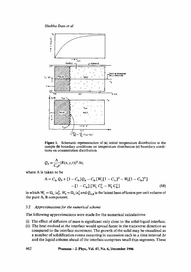
The experimental conditions compatible with these boundary conditions are shown schematically in figures l(a, b, c). The sample is considered to be semi infinite on which an exponential external temperature gradient is maintained in the x direction. These boundary conditions are the same as selected by Chvoj [37] for his two dimensional ( 1-space, 1 -time) model.

Equations (66) and (67) together with (47) and (48) are numerically solved for C L and T respectively using finite difference method [44] and an iterative scheme, namely, the successive overrelaxation method (SOR) [45].

The position of the solid-liquid interface is denoted by delta function in the present model. As the solidification process proceeds latent heat is evolved at the interface X~(y,t) giving rise to the source term Qr in (67). The delta function is taken into account such that the heat evolved in time At is equal to the latent heat for the volume R A t solidified in the time At and is given by


Shobha Dass et al

" - -> X(a )

$AMPL[ --7 ~-- FURNACE

• AXIS OF SYMMETRY T I - ( i t ~F "MELT " IN y OIRECTIDN

T 2

V,O x:o (b)

. " CLO

MELT.

CLOCLOJ C//~a: ~ (c)~ ~x'

: -D~ ( CL°-Csr )

T 2

Figure 1. Schematic representation of (a) initial temperature distribution in the sample (b) boundary conditions on temperature distribution (e) boundary conditions on concentration distribution.

A QT = ~-~-" (R(x, y, t)) 2 At,

LvP

where A is taken to be

A = Csr Qa + [1 - Csr ] QA - - Csri-WL [1 - - CL,] 2 - Ws[1 - Cs~] 2]

- [1 - Csr ] [WE CLZ,- Ws Cs~] (68)

in which W L ~-~L / a3, Ws 3 = = t) s/a o and QA,B is the latent heat of fusion per unit volume of the pure A, B component .

3.2 Approximat ions for the numerical scheme

The following approximations were made for the numerical calculations:

(i) The effect of diffusion of mass is significant only close to the solid-liquid interface. (ii) The heat evolved at the interface would spread faster in the transverse direction as

compared to the interface movement. The growth of the solid may be visualized as a number of solidification events occurring in succession each in a time interval At and the liquid column ahead of the interface comprises small thin segments. These

462 Pramana - J. Phys., VoL 47, No. 6, December 1996


segments of the system close to the interface stabilizes in the time interval At and steady-state equations can be used to express the process during At.

(iii) Initial stage of phase transformation i.e. the nucleation process is not considered and the growth is continuous.

(iv) The total domain is divided into two regions, the interface region and the liquid phase. Interface is considered as one of the boundaries moving with time. It is further assumed that the interface temperature at time t constitutes the boundary temperature at time t + At.

(v) Interface concentrat ion CLr in the flux condition is approximately equal to the equilibrium concentrat ion CLO.

3.3 System studied and computer software

The values of the thermophysical properties chosen (table 1) in the present calculations do not correspond to any particular material but they are close to the typical values of many materials, for example Cu-Ni , C u - A g etc. [40]. The two components considered here have the same crystal structure (FCC) and they do not exhibit any solid-state allotropic transformations. The interactions parameters f~L and f~s are taken independent of temperature.

The numerical scheme was applied to six different systems having interaction parameters

System I D E = 2"8 x 10 - 2 0 J/atom System II ~'~L = 2"8 x 10 - 2 1 J/atom System II I ~r'~ L = 2"8 X 10- 19 J/atom System IV D E = - 2.33 x 10 -20 J /atom System V ~r'~ L -~- -- 2"8 X 10 - 2 0 J/atom System VI ~')L = -- 2"8 X 10-20 J/atom

Table 1. Values used [33, 48].

f~s = 2"33 x 10 -20 J /a tom D. s = 2-8 x 10-20 J /a tom f~s = 2.8 x 10 -20 J /a tom f~s = - 2.47 x 10 - 2 0 J /a tom fls = - 2-8 x 10-19 J /a tom f~s = - 2-8 x 10 - 2 1 J /a tom

of thermophysical parameters

Constant Numerical value Units

AHA 2-12 x 10 -20 J/atom AH B 3-11 x 10 -20 J/atom a o 0-36 x 10 -9 m T A 1360 K T B 1730 K K B 1"38 × 10 -23 J/K T 2 1997 K U 0"5 x 10-t9 j v 3 x 101° s - t D c 0"73 x 10 -7 m2/s Dr 5"8 x 10-s m2/s k 200 J/s/m/K (o 0.001 m QA - 1"82 x 109 J / m 3 Qa - 2.67 x 109 J / m 3


Shobha Dass et al

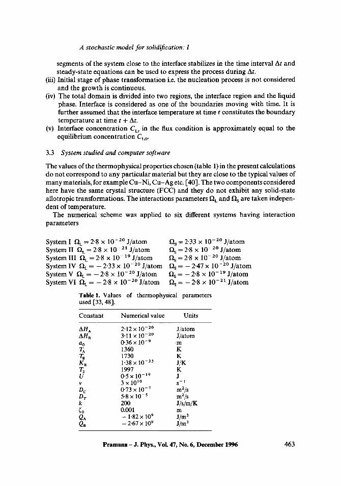
Each system was studied for 5 to 9 different sets of initial values of equilibrium concentration CLO and temperature T~. Values of CLo, T1 and ~b lies between 0-02-0-98, 1190 K-1703 K and 105-0.5 x 108 K/s respectively. Width of the sample was taken to be 10- s m. It facilitates the construction of nonequilibrium phase diagrams and the study of their time evolution.

A computer program was written in Basic Language and calculations were per- formed on PC-AT286 at the Department of Physics and the University Computer Centre of Rani Durgavati University and Govt. M.H. College of Science and Home Science, Jabalpur. 100 points on x axis, which is the direction of the external temperature gradient, 20 points on y axis and 5-10 points on t axis were taken. The total computational run time lies between 3 to 7 h for each set of values of initial concentration and temperature. The length of the solid formed lies between 5-1 x 10 -7m to 6 x 10-5m for the total evolution time 0-28 x 10-Ss and 10-3s respectively. The accuracy in the convergence criterion was chosen to be 1%.

4. Results and discussion

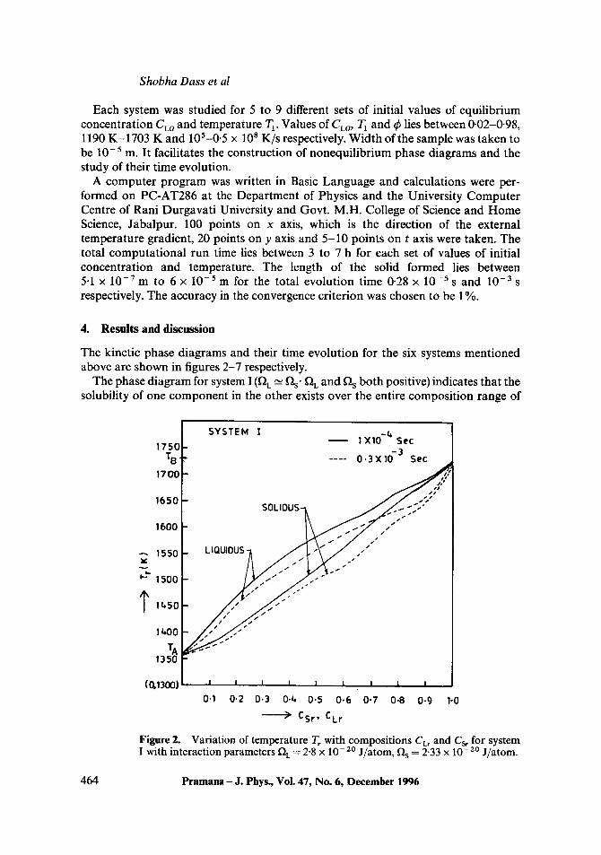
The kinetic phase diagrams and their time evolution for the six systems mentioned above are shown in figures 2-7 respectively.

The phase diagram for system I (QL ~ Qs" QL and Qs both positive) indicates that the solubility of one component in the other exists over the entire composition range of

1700

1650

1600

1550 ~ 1500 11,50

1~00

TA 1350

(0,1300)

Figure 2.

SYSTEM I 1 XIO -~ Sec

-3 . . . . 0.3X10 Sec ,/

/ / / ,,'S

/ / / / / I / /

I I I I I I I I I

0.1 0.2 0.3 0-~, 0.5 0.6 0.7 0.8 0-9 1-0

> CSr, CLr

Variation of temperature T, with compositions CL, and Cs, for system I with interaction parameters f]L = 2"8 x 10 - 2 0 J/atom, D. s = 2.33 x 10 - 2 0 J/atom.

464 Pramana - J. Phys., VoL 47, No. 6, December 1996


SYSTEM II 13.50

-- ~X10 -s Sec 1300

. . . . 2.8X i0" ~'sec 1250

1 2 0 0 - I . . i / r LIOUIOUS FSOLIOUS / /

'- , , oo -__X / \ > 4 " . - " " I .-" 1" \ / I A " / , ' "

~oso- -,, ",X,. \ / ,I ~ /" I -\ , x . . . ~ \ / ~ \ /- . \ ~ -'..a,,r--¢~ t ." ,ooo ,,,,,.----,,-7-,, 3-

9SO t "", ~', ...~/....- [ ~ - ' " l O , g o 0 ) l I I l i I i I I i

(3.1 0-2 0.3 0.(~ 0.5 0-6 0.7 O.B 0.9 1.0

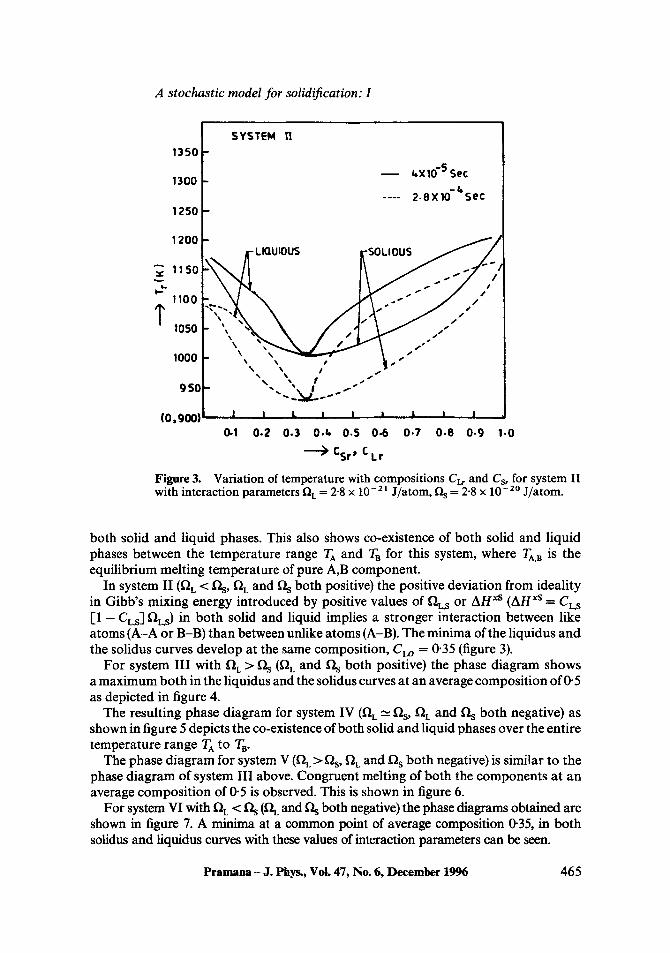
) Csr) C Lr Figure 3. Variation of temperature with compositions CLr and Cs, for system II with interaction parameters ~C = 2"8 X 10 -21 J/atom, f~s = 2"8 x 10 -20 J/atom.

both solid and liquid phases. This also shows co-existence of both solid and liquid phases between the temperature range T A and T B for this system, where TA, B is the equilibrium melting temperature of pure A,B component.

In system II (f~L < D's, f~L and D. s both positive) the positive deviation from ideality in Gibb's mixing energy introduced by positive values of f~L.S or AH xs (AH xs = CL, s [1 -- CL,s_ ] IlL,S) in both solid and liquid implies a stronger interaction between like atoms (A-A or B-B) than between unlike atoms (A-B). The minima of the liquidus and the solidus curves develop at the same composition, CLO = 0"35 (figure 3).

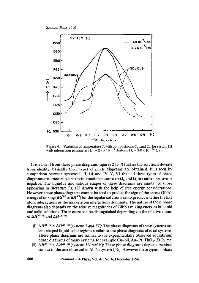
For system III with f~t > flS (~-~L and D. s both positive) the phase diagram shows a maximum both in the liquidus and the solidus curves at an average composition of 0"5 as depicted in figure 4.

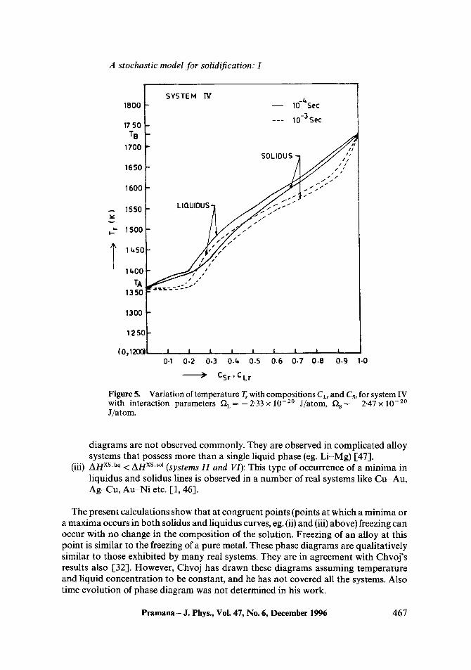
The resulting phase diagram for system IV (Dr "-" f~s, f~L and f~s both negative) as shown in figure 5 depicts the co-existence of both solid and liquid phases over the entire temperature range T A to T B.

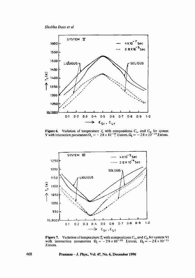
The phase diagram for system V (Dr >f2 s, f2 L and f2 s both negative) is similar to the phase diagram of system III above. Congruent melting of both the components at an average composition of 0"5 is observed. This is shown in figure 6.

For system VI with f~L < D~ (D r and ~ both negative) the phase diagrams obtained are shown in figure 7. A minima at a common point of average composition (~35, in both solidus and liquidus curves with these values of interaction parameters can be seen.

Pramana - J. Phys., VoL 47, No. 6, December 1996 465

Shobha Dass et al

1550

1525

1500

1 G75

T~,50

1~25

I~OC

1375 t / 1350 / /

(0,1300) " ' 0"1

SYSTEM IIl m t~X to-Tsec.

~ ___ 3.2X10"Gsec

/ / \

/ \ \ f ~

I I i I I I I I

0.2 0"3 O.t~ 0"5 0"6 0-7 0"8 0.9 1.0 > CSr, CLr

Figure 4. Variation of temperature T, with compositions Cgr and Csr for system III with interaction parameters f~L = 2"8 X 10- 19 J/atom, Ds = 2"8 x 10- 20 J/atom.

It is evident from these phase diagrams (figures 2 to 7) that as the solutions deviate from ideality, basically three types of phase diagrams are obtained. It is seen by comparison between systems I, II, III and IV, V, VI that all three types of phase diagrams are obtained when the interaction parameters f~L and ~s are either positive or negative. The liquidus and solidus shapes of these diagrams are similar to those appearing in literature [-1, 12] drawn with the help of free energy considerations. However, these phase diagrams cannot be used to predict the sign of the excess Gibb's energy of mixing (AG xs "~ AH xs) for the regular solutions i.e. to predict whether the like atom interactions or the unlike atom interactions dominate. The nature of these phase diagrams also depends on the relative magnitudes of Gibb's mixing energies in liquid and solid solutions. Three cases can be distinguished depending on the relative values of AH xs'liq and AH xs''°l.

(i) A n Xs'liq "~ AH xs''°l (systems I and I V): The phase diagrams of these systems are lens shaped liquid-solid regions similar to the phase diagrams of ideal systems. These phase diagrams are similar to the experimentally observed equilibrium phase diagrams of many systems, for example Cu-Ni, Au-Pt, ThO2-ZrO 2 etc.

(ii) AH xsAiq > AH xs'°~ (systems III and V): These phase diagrams depict a maxima similar to the one observed in A1-Ni system [-46]. However these types of phase

4 6 6 Pramana - J. Phys., Vol. 47, No. 6, December 1996


SYSTEM IBO0

17 50 T B

1700

1650

1600

1550 LIoUIOUS-

1500

I 1 t b 5 0 ~ / / ¢

lt~O0 ~ A / °J

1350 F

1300 F

12 SO F (0,1200)/ I 1 I

0.1 0.2 0.3

>

_ _ lO-~Sec

___ 10-3 Sec

,el / 1

SOLIDUS / y / ¢ ; I r

I I l I I I

O.t~ 0.5 0.6 0.7 0.8 0.9 1-0 CSr, C Lr

Figure 5. Variation of temperature T, with compositions CLr and Cs, for system IV with interaction parameters I)L=--2'33 x 10 -20 J/atom, ~s = --2.47x 10 -20 J/atom.

diagrams are not observed commonly. They are observed in complicated alloy systems that possess more than a single liquid phase (eg. Li-Mg) 1-47].

(iii) AH xstlq < AH xs's°l (systems II and VI): This type of occurrence of a minima in liquidus and solidus lines is observed in a number of real systems like Cu-Au, Ag-Cu, Au-Ni etc. [1, 46].

The present calculations show that at congruent points (points at which a minima or a maxima occurs in both solidus and liquidus curves, eg. (ii) and (iii) above) freezing can occur with no change in the composition of the solution. Freezing of an alloy at this point is similar to the freezing of a pure metal. These phase diagrams are qualitatively similar to those exhibited by many real systems. They are in agreement with Chvoj's results also [32]. However, Chvoj has drawn these diagrams assuming temperature and liquid concentration to be constant, and he has not covered all the systems. Also time evolution of phase diagram was not determined in his work.


Shobha Dass et al

1600

1550

1500

1~50

,- I~00

t 1350

1300

12so

(0,1200) !

! SYSTEM y

LI~UIDUS-

t~XlO- 7Sec

--- 2.8 X 10- 6Sec

/lisp p • I / S #p~/s I I I I I

0-I 0.2 0.3 0-~ 0-5

~ s S ! ~ / %

t

-SOLIDUS

I I I I 0.6 0-7 0-8 0-9 1-0

) CSr , C Lr

Figure 6. Variation of temperature T, with compositions CL, and Cs~ for system V with interaction parameters f~L = -- 2"8 X 10- 20 J/atom, D, s = - 2-8 x 10-19 J/atom.

1250

1200

1150

v 1100

SYSTEM ' ~ 4XlO-5Sec

. . . . 2.B X lO-b'Sec

-LIOUIOUS S O L I D U S U ~ / . , s

. " s I

i I I J I s s l

f l J t i050 1 "

I000 r " "

I g50 I

( o , g o o ) t L , i , '

0.I 0.2 0.3 O.L, 0-5 0.6 0.7 0.8 0.9 1.0

~" Csr , C Lr

Figure 7. Variat ion of temperature T~ with composi t ions CLr and Csr for system VI with interact ion parameters fiE = - -2"8X10 - z ° J / a tom, fls = - - 2 " 8 x 1 0 -21 J /a tom.

I | I I



Figures 2-7 also show the time evolution of phase diagrams. It can be seen from these figures that the phase diagrams shift towards the lower temperature region with time and only a slight change in the shape is observed. Large changes in the shape are not obtained presumably due to the assumption of the linear relationship between currents and gradients, which implies that the system is not very far from equilibrium. Also, the total time elapsed, which has been considered in the calculations is small (10- 5_10- 3 s). This was due to the limitations of the computational time and the numerical scheme.

5. Conc lus ions

The stochastic model in 3-dimensions (2-space, 1-time) presented here is suitable to study solidification of materials in general, depending on their thermophysical properties. The merit of this model lies in the fact that the growth not necessarily restricted to near equilibrium conditions can also be taken into account. During the nonequilibrium solidification the concentrations of solid and liquid phases, rate of growth, undercool- ing and the boundary conditions vary with time. These variations are included in this model, enabling the determination of the composition and microstructure of the new phase. Also, interdependence of temperature and concentration together with the effect of kinetic processes at the solid-liquid interface are included in this model. The various approximations can easily be relaxed in this model.

This study is important from the point of view of predicting the outcome of experiments to produce materials with desired and reproducible properties. In order to explain other type of nonequilibrium phase diagrams and microstructures observed, this model can be further extended to multi component systems and 4-dimensions (3-space, 1-time). Also, other type of boundary conditions representing different growth techniques can be studied. This model has been applied to binary alloys having wide range of typical thermodynamic parameters and the kinetic phase diagrams have been obtained. The study of interface movement, shape etc. are given in part II of this paper.

A c k n o w l e d g e m e n t s

One of the authors (LP) is thankful to Prof. P Ramachandrarao for many stimulating discussions. Financial assistance by the University Grants Commission in the form of teacher fellowship to SD is gratefully acknowledged.

References

[1] F C Flemings, in Solidification processing (Mc-Graw Hill Inc., New York, 1974) [2] W Kurz and D J Fisher, in Fundamentals of solidification (Trans-Tech Publication,

Switzerland, 1986) [3] P Strimbord, D R Nelson and M Roucheti, Phys. Rev. Lett. 47, 1297 (1981) [4] P Ramachandrarao, G V S Shastri, L Pandey and A Sinha, Acta, Cryst. A47, 206 (1991) [5] D Domb and J L Lebowitz (eds.) in Phase transitions and critical phenomena. (Academic,

London, 1983) [6] N Sounders and A P Miodownik, J. Mater. Res. 1, 1803 (1986) [7] F X Kelly and L H Ungar, Phys. Rev. B. 34, 1746 (1986) [8] Z Chvoj, Z Kozisek and J Sestak, Thermochim. Acta. 153, 349 (1989)

Pramana - J. Phys., Voi. 47, No. 6, December 1996 469

Shobha Dass et al

[9] D T Gillespie, J. Chem. Phys. 74, 661 (1981) [10] D Kashchiev, Cryst. Res. Tech. 19, 1413 (1984) [11] A K Ray, M Chalom and L K Peters, J. Chem. Phys. 85, 2161 (1986) [12] P Gordon, in Principles of phase diayrams in materials (Mc-Graw Hill, 1968; Jersey, 1972) [13] A K Jena and M C Chaturvedi, in Phase transformation in materials. (The Metals Society,

Eaglewood Cliffs, New Jersey 1992) [14] A Bruce and D Wallace, Phys. Rev. Lett. 4, 457 (1982) [15] J S Langer and L A Turski, Phys. Rev. A8, 3230 (1973) [16] J S Langer and A J Turski, Phys. Rev. A22, 2189 (1980) [17] J S Langer and A J Swartz, Phys. Rev. A21, 948 (1980) [18] V P Skripov and A V Skripov, Usp. Fiz. Nauk. 128, 193 (1979) [19] V P Skripov and V P Koverda, in Spontaneous crystallization of undereooled liquids

(Nauka, Moscow, 1984) [20] A D J Haymet and D W Oxtoby, J. Chem. Phys. 84, 1769 (1986) [21] A D J Haymet, Pro9. Solid State Chem. 17, 1 (1986) [22] B B Mandelbrot, in Thefractal 9eometry of nature (Freeman, San Francisco, 1982) [23] D S Cannel and C Aubert, in Fractal and non fractal patterns in physics, in 9rowth and form

edited by H E Stanley and N Ostrowski (Martinus Nijhoff, Dordrecht, 1986) [24] B Caroli, C. Caroli and B J Roulet, J. Cryst. Growth 66, 575 (1984) [25] T A Cherepanova, J. Cryst. Growth 59,371 (1980) [26] T A Cherepanova, Phys. Status. Solidi A58, 469 (1980) [27] T A Cherepanova, J. Cryst. Growth 52, 319 (1981) [28] L Pandey and P Ramachandrarao, Acta. Metall. 35, 10, 2549 (1987) [29] R Trivedi, P. Magnin and W Kurz, Acta Metall. 35, 971 (1987) [30] G S Reddy and J A Sekhar, J. Mater. Sci. 21, 3535 (1985) [31] Z Chvoj, Czech. J. Phys. B37, 1256 (1987) [32] Z Chvoj, Cryst. Res. Tech. 21, 8, 1003 (1986) [33] Z Chvoj, Czech. J. Phys. B37, 607 (1987) [34] Z Chvoj, Czech. J. Phys. B33, 961 (1983) [35] Z Chvoj, Czech. J. Phys. B33, 1060 (1983) [36] Z Chvoj, Czech. J. Phys. B34, 548 (1984) [37] Z Chvoj, Czech. J. Phys. B36, 863 (1986) [38] Z Chvoj, Czech. J. Phys. B37, 1340 (1987) [39] Z Chvoj, Czech. J. Phys. B40, 473 (1990) [40] Z Chvoj, Czech. J. Phys. B40, 483 (1990) [41] S Dass, G Johri, L Pandey and P Ramachandrarao, in II Annual General Meetin9 of MRSI

held at NPL, New Delhi, February 9-10 (1991) [42] C W Gardiner, in Handbook of stochastic methods (Springer-Verlag, Berlin, 1985) [43] C N R Rao and K J Rao, in Phase transitions in solids (Mc-Graw Hill, Chatham, 1978) [44] J B Scarborough, in Numerical mathematical analysis (Oxford and IBH Publishing Co.,

New Delhi, 1976) [45] M Krizek and P Neittaanmaki, in Finite element approximationof variational problems and

applications (Longman Scientific with John Wiley Inc., New York, 1990) [46] B Chalmers, in Principles of Solid!fication (John Wiley and Sons, New York, 1967) p.7 [47] R E Reed-Hill, in Physical metallurgy principles (EWP, New Delhi, 1975) p. 535 [48] R C Weast (ed.) CRC Handbook of Chemistry and Physics, (CRC Press Inc., 1988)

4 7 0 Pramana - J. Phys., Vol. 47, No. 6, December 1996