A Stochastic Supply/Demand Model for

Storable Commodity Prices

ALI BASHIRI and YURI LAWRYSHYN

ABSTRACT We develop a two-factor mean reverting stochastic model for forecasting storable commodity prices

and valuing commodity derivatives. We define a variable called “normalized excess demand” based on

the observable production rate, consumption rate, and inventory levels of the commodity. Moreover,

we formulate and quantify the impact of this factor on the commodity spot and futures prices. We apply

this model to crude oil prices from 1995 to 2016 via a Kalman filter. Our analysis indicates a strong

correlation between normalized excess demand and crude oil spot and futures prices. We analyze the

term structure of futures prices under the calibrated parameters as well as the implications of changes in

the underlying factors.

I. Introduction Commodities are an integral part of the global economy. Economies of both producing and consuming

nations are vastly affected by commodities' prices. For instance, Hamilton (2008) and Morana (2013)

demonstrate that oil price increase has preceded nine out of ten most recent US recessions. Hamilton

(2011) and Cuñado & Gracia (2003) show the detrimental effects of oil price shocks on US and

European Economies. The importance of commodities to national security has prompted governments

and financial markets to pay close attention to commodities' price levels. Commodity pricing plays an

important role in real options valuation. Kobari et al. (2014) demonstrate the importance of oil prices in

the real options valuation, operational decisions, and expansion rate of Alberta oil sands projects.

Bastian-Pinto et al. (2009) demonstrate the impact of sugar and ethanol price processes on the real

option valuations of ethanol production from sugarcane. Brandão et al. (2013) show the significance of

the soybean and castor bean price processes for real options valuation of managerial flexibility

embedded in a biodiesel plant.

Moreover, in recent decades, commodities have become an investment asset in financial portfolios

providing protection against inflation and as a diversifying factor, boosting portfolios' risk-reward

profiles (Geman 2005; Gorton & Rouwenhorst 2006). Juvenal & Petrella (2015) estimated that assets

allocated to commodity index trading had increased from $13 billion in 2004 to $260 billion in 2008.

Importance and widespread use of commodities has led to growth of variety and trading volume of

financial products related to commodities. According to statistics published by the Bank for

International Settlements (Semiannual OTC derivatives statistics), notional value of over-the-counter

commodities’ derivatives increased from $415 billion in 1998 to over $2 trillion in 2015. The increase

in trading volume and importance of commodities in real project / option valuation has made the

pricing of commodity products a priority.

Commodity prices exhibit stochastic behavior. Many factors contribute to the pricing of commodity

related financial products. The majority of previous literature has either focused on modeling

stochasticity of the prices or finding causal links between commodities' prices and a range of

commodity specific and economic factors.

Gibson & Schwartz (1990), Schwartz (1997), Casassus & Collin-Dufresne (2005), Hikspoors &

Jaimungal (2008), Trolle & Schwartz (2009), Liu & Tang (2011), Chen & Insley (2012), Mirantes,

Población, & Serna (2013), and Lai & Mellios (2016) are some recent examples of literature focused

on modeling stochasticity of commodity prices, convenience yield, interest rates, and volatility.

Schwartz (1997) is a seminal work on the modeling mean reversion and stochasticity of commodity

prices. Routledge et al. (2000) is an influential work on modeling term structure of forward prices in

equilibrium. In this work, the impacts of changes in inventory, net demand shocks, and convenience

yield on forward prices are discussed. They show convenience yield is a results of interaction between

supply, demand, and inventory.

Another category of literature is concerned with analyzing the effects of commodity prices on

commodity-specific and economic factors. Commodity specific factors are factors directly affecting the

production and consumption of commodities, such as supply, demand, inventory levels, and even

geopolitical tensions in the case of energy products. Güntner (2014) analyzes the impact of oil prices

and demand on oil production within OPEC and non-OPEC producers. Bu (2014) shows that weekly

inventory data published by the U.S. Energy Information Agency (EIA) has a significant impact on oil

prices.

Alternatively, economic factors indirectly impact commodity prices by changing the expected supply

and demand for commodities. For instance, global economic activity is expected to have an impact on

global energy demand. Kaminski (2014) classifies the North American energy market’s determinants

as physical, financial, and socioeconomic layers, and measures their impacts on the market. Stefanski

(2014) analyzes the impact of structural changes in the industrialization level of developing countries

on the energy markets.

Employing an econometric approach, Kilian’s work demonstrates the importance of supply, demand,

and inventory levels on commodity prices within a vector autoregressive model. Kilian & Lee (2014)

analyze the impact of speculative demand shocks on oil prices. Kilian (2014) demonstrates that supply

and demand levels are integral parts of oil price dynamics. Baumeister & Kilian (2016) create a vintage

dataset consisting of global oil production, US and OECD oil inventory levels and other factors, and

demonstrate improved forecasting capabilities compared to similar vector autoregressive models.

The literature demonstrates strong evidence of stochasticity of the commodities' prices, convenience

yield, and volatility. Moreover, literature also suggests strong explanatory power of production,

consumption, and inventory levels. In this work, we propose a two-factor stochastic model

incorporating commodities’ prices as well as supply, demand, and inventory data.

In the equilibrium setting, commodity prices should follow a mean reverting process. With increasing

price, supply of the commodity will increase as higher marginal cost producers enter the market. This

increase in supply will in turn reduce the demand pressure on the price and slow or reverse the price

increase. Conversely, with a decrease in price, higher marginal cost producers would halt production.

The lower supply of the commodity would reduce the downward pressure on the price and slow the fall

in production rates, resulting in an upward price pressure. Thus, in equilibrium, commodity prices are

expected to follow a mean reverting process. Schwartz (1997) models commodity prices via an

Ornstein-Uhlenbeck process reflecting this mean reverting dynamic.

In this work, we propose a two factor stochastic model. The first factor is the commodity’s spot price

and the second factor is the normalized excess demand for the commodity. This model is unique in

that it proposes a mean reverting factor related to supply, demand, and inventory levels and measures

the impact of changes in these variables on the commodity prices. Moreover, it is calibrated not only on

the commodity prices, but also on the observable supply, demand, and inventory levels. This model is

then applied to oil markets. Following the Schwartz (1997) framework, since the spot price,

supply/demand, and inventory data of commodities are uncertain and unobservable, we use oil futures

prices for model calibration. Specifically, the model is put in a state-space form and a Kalman filter is

applied to estimate the model parameters and values of the state parameters. We apply the model to oil

market data from 1996 to present time. We use the West Texas Intermediate (WTI) futures data on a

monthly basis as well as quarterly data on supply, demand, and inventory published by the

International Energy Agency (IEA).

The remainder of this work is organized as follows. Section 2 explains the economic rationale for the

model. In Section 3, the forecasting model is explained and reviewed. In Section 4, the data is

presented and described. Section 5 explains the calibration methodology. Section 6 presents results of

the model calibration and forecasting. Finally, Section 7 presents the concluding remarks.

II. Economic Rationale In this section, we will discuss the economic rationale behind the proposed model. As mentioned in the

introduction, commodity spot prices are often modeled as mean reverting processes. With increasing

demand, commodity prices increase as well. The increase in price leads to an increase in supply as

producers with higher production costs enter the market. The increase in supply, in turn, balances the

excess demand and leading to increasing price levels. In reverse, with increasing excess supply, the

prices fall to reflect the abundance of the commodity. Falling prices then push out the producers with

higher production cost and reduce the excess demand and balance the price. In this version of mean

reversion, every price increase is followed by a price fall and every price decrease is followed by a

price rise due to a balancing process between supply and demand.

In this work, we propose a different mean reverting model for commodities. We postulate that

commodity spot prices grow exponentially at a rate dependent on various factors such GDP growth

rate, inflation, and other market factors. For instance, as GDP increases, price levels in both financial

and physical markets have to grow to accommodate both producers and consumers. Chiang et al.

(2015) conclude that oil prices have a statistically significant and economical relationship with real

GDP. Another factor is inflation. Inflation leads to devaluation of currencies. A unit of a given

commodity and costs associated with production of that unit do not decrease with the unit of currency.

This leads to an increase in the nominal value of a unit of commodity as inflation devalues the

currency. Szymanowska et al. (2014) find evidence of sizeable impact of inflation as well other factors

on spot and term risk premia for a high-minus-low portfolio of seven commonly used commodities

ranging from energy to agricultural products and industrial metals. Moreover, commodities returns are

shown to be positively correlated with inflation (Greer 2000; Erb & Harvey 2006; Gorton &

Rouwenhorst 2006).

Finally, we believe commodities are impacted by supply, demand, and inventory levels observable by

the market. A positive demand shock (negative supply shock) would increase the price of the

commodity while a negative demand shock (positive supply shock) would decrease the price. However,

it is not the absolute demand or supply shock that would impact the price but the relative value of the

shock. For instance, if the positive shock in demand is followed by a positive shock in supply, the value

of the commodity should not be impacted by the shocks as increasing supply would offset increasing

demand. Moreover, inventories act as a buffer for the markets by absorbing excess supply and

offsetting excess demand. However, it should be noted that inventories only provide buffering capacity

for storable commodities (see Routledge et al. 2000; Carlson et al. 2007; Sockin & Xiong 2015 for

discussion on impacts of inventory on storable commodities). Moreover, inventories cease to provide

buffering protection for positive supply shocks at near maximum capacity. This is due to limited

capacity for storage and not being able to mix different qualities of a commodity such as crude oil in

the same container (Kaminski 2014). We propose a ratio called “normalized excess demand” and

defined as

𝑞 =

𝐷 − 𝑆 − 𝐼

𝐷, (1)

to represent the impact of supply, demand, and inventory on commodity spot prices. Here D, S and I

represent observable demand, supply and inventory of the commodity. We postulate that this ratio

follows a mean reverting process. In the long term, there should be a balance between supply, demand,

and inventory levels. Supply and inventory levels should always be in line with demand. Therefore, the

ratio of excess total supply to demand should be mean reverting in the long term. Deviation from this

long term mean level would have an impact on prices. With increasing total supply, this ratio would

decrease and in turn, prices would decrease. We formulate the model such that this ratio impacts the

growth rate of spot prices through a convenience yield factor defined as

𝛿 = 𝑎𝑞 + 𝑏, (2)

where a and b are constants that can be fitted to data. For instance, with increasing supply, the

normalized excess demand factor would decrease. Producers and market participants are expected to

store the commodity at this point. It is then expected that the convenience yield would increase

providing incentive for participants to store the commodity. The increase in convenience would also

reduce the growth rate of spot prices and even reduce the prices if the magnitude of the supply increase

is significant. In the next section, details of the proposed model are presented.

III. Model This section outlines the proposed model and derivatives’ valuations. The two factors of this model are

the spot price, S, and the normalized excess demand of the commodity, q. The two factors are modeled

as the following joint stochastic processes:

𝑑𝑆

𝑆= (µ − 𝛿)𝑑𝑡 + 𝜎𝑠𝑑𝑧𝑠 , (3)

𝛿 = 𝑎𝑞 + 𝑏, (4)

𝑑𝑞 = 𝜅(𝜃 − 𝑞)𝑑𝑡 + 𝜎𝑞𝑑𝑧𝑞 , (5)

where,

- µ is the drift of the prices based on macroeconomic factors such as GDP and Inflation

- 𝛿 is the convenience yield,

- 𝜎𝑠 is the volatility of the oil prices,

- 𝑍𝑠 is a standard Brownian motion,

- 𝑎 and 𝑏 are the constants relating normalized excess demand to convenience yield,

- 𝜅 is the rate of mean reversion,

- 𝜃 is the level of mean reversion,

- 𝜎𝑞 is volatility of the normalized excess demand, and

- 𝑍𝑞is a standard Brownian motion,

and the two standard Brownian motions are correlated as

𝑑𝑧𝑠𝑑𝑧𝑞 = 𝜌𝑑𝑡, (6)

where 𝜌 is the correlation between the two motions.

Equation (3) models the spot process of the commodity as a geometric Brownian motion (GBM)

including a convenience yield term incorporating the benefits of storage to commodity holders in favor

of consuming the commodity. Equation (4) describes the convenience yield process related to the

normalized excess demand factor. Equation (5) describes the normalized excess demand process.

Normalized excess demand (q) is modeled as an Ornstein-Uhlenbeck mean reverting stochastic

process. As already mentioned, the normalized excess demand is defined as

𝑞 =

𝐷 − 𝑆 − 𝐼

𝐷, (7)

where D is market demand, S is supply, and I is the inventory level per day.

Following standard transformation and applying Ito’s Lemma, the spot process can be defined in

logarithm form as

𝑑𝑋 = (µ − 𝛿 −

𝜎𝑠2

2) 𝑑𝑡 + 𝜎𝑠𝑑𝑧𝑠 , (8)

where 𝑋 = log (𝑆).

Under the risk-neutral framework, applying the Girsanov’s theorem, the model can be presented as

𝑑𝑋 = (𝑟 − 𝛿 −

𝜎𝑠2

2) 𝑑𝑡 + 𝜎𝑠𝑑𝑧𝑠∗

, (9)

𝛿 = 𝑎𝑞 + 𝑏, (10)

𝑑𝑞 = [𝜅(𝜃 − 𝑞) − 𝜆]𝑑𝑡 + 𝜎𝑞𝑑𝑧𝑞∗, (11)

𝑑𝑧𝑠∗𝑑𝑧𝑞∗ = 𝜌𝑑𝑡, (12)

where,

- 𝑍𝑠∗ and 𝑍𝑞∗

are standard Brownian motions under the equivalent risk-neutral measure, and

- 𝜆 is the market price of risk.

This joint distribution for log-spot price and normalized excess demand can be then presented as

(

𝑋(𝑡)

𝑞(𝑡)) ~𝑁 ([

𝜇𝑋

𝜇𝑞] , [

𝜎𝑋2 𝜎𝑋𝑞

𝜎𝑋𝑞 𝜎𝑞2 ] ), (13)

where 𝑁(∙) represents a bivariate normal distribution, the terms 𝜇𝑋, 𝜇𝑞, 𝜎𝑋2, 𝜎𝑞

2, and 𝜎𝑋𝑞are derived in

Appendix A and defined as

𝜇𝑋 = 𝑋0 + (𝜇 −

1

2𝜎𝑠

2 − 𝑎𝜃 − 𝑏) 𝑡 −𝑎

𝜅(𝑞0 − 𝜃)(1 − 𝑒−𝜅𝑡), (14)

𝜇𝑞 = 𝑞0𝑒−𝜅𝑡 + 𝜃(1 − 𝑒−𝜅𝑡), (15)

𝜎𝑋

2 = 𝜎𝑠2𝑡 +

𝑎2𝜎𝑞2

𝜅2[𝑡 +

(1 − 𝑒−2𝜅𝑡)

2𝜅−

2(1 − 𝑒−𝜅𝑡)

𝜅] −

2𝑎𝜎𝑠𝜎𝑞𝜌

𝜅[ 𝑡 −

(1 − 𝑒−𝜅𝑡)

𝜅], (16)

𝜎𝑞

2 =𝜎𝑞

2

2𝜅(1 − 𝑒−2𝜅𝑡), (17)

𝜎𝑞

2 =𝜎𝑞

2

2𝜅(1 − 𝑒−2𝜅𝑡). (18)

Applying the Feynman-Kac theorem, any derivative under this model should satisfy the following

partial differential equation for undiscounted derivatives (g)

𝑔𝑡 + (𝑟 − 𝛿)𝑆𝑔𝑆 + [𝜅(𝜃 − 𝑞) − 𝜆]𝑔𝑞 +

1

2𝜎1

2𝑆2𝑔𝑆𝑆 + 𝜎1𝜎2𝜌𝑆𝑔𝑆𝑞 +1

2𝜎2

2𝑔𝑞𝑞 = 0, (19)

and the following PDE for discounted derivatives (f)

𝑓𝑡 + (𝑟 − 𝛿)𝑆𝑓𝑆 + [𝜅(𝜃 − 𝑞) − 𝜆]𝑓𝑞 +

1

2𝜎1

2𝑆2𝑔𝑆𝑆 + 𝜎1𝜎2𝜌𝑆𝑓𝑆𝑞 +1

2𝜎2

2𝑓𝑞𝑞 = 𝑟𝑓. (20)

As previously mentioned, we use futures data for calibration of this model. For a futures contract, the

PDE in equation (19) is subject to terminal condition 𝐹𝑇 = 𝑆. A futures contract’s value at time t with

maturity 𝜏 = 𝑇 − 𝑡 is obtained as the expectation of the spot price at maturity. Given the log-normal

distribution of spot price, we have

𝐹(𝑆𝑡, 𝑞𝑡, 𝜏) = EQ[𝑆𝑇] = e

𝜇𝑋𝑄

+0.5𝜎𝑋2

, (21)

where 𝜇𝑋𝑄

is the mean of log-spot price under the risk-neutral measure derived as

𝜇𝑋

𝑄 = 𝑋0 + (𝑟 −1

2𝜎𝑠

2 − 𝑎𝜃 − 𝑏 +𝑎𝜆

𝜅) 𝑡 −

𝑎

𝜅(𝑞0 − 𝜃 +

𝜆

𝜅) (1 − 𝑒−𝜅𝑡). (22)

Substituting for 𝜇𝑋𝑄

and 𝜎𝑋2 in equation (21) and reorganizing the equation, we can obtain

𝐹(𝑆𝑡, 𝑞𝑡 , 𝜏) = 𝑆𝑡𝑒𝐴(𝜏)+𝐵(𝜏)𝑞𝑡 , (23)

where,

𝐴(𝜏) = (𝑟 − 𝑎𝜃 − 𝑏 −

𝑎𝜎𝑠𝜎𝑞𝜌

𝜅+

𝑎2𝜎𝑞2

2𝜅2) 𝜏 + (𝑎𝜃 +

𝑎𝜎𝑠𝜎𝑞𝜌

𝜅−

𝑎2𝜎𝑞2

𝜅2)

(1 − 𝑒−𝜅𝜏)

𝜅+

𝑎2𝜎𝑞2

4𝜅3(1 − 𝑒−2𝜅𝜏), (24)

𝐵(𝜏) = −

𝑎(1 − 𝑒−𝜅𝜏)

𝜅, (25)

𝜃 = 𝜃 −

𝜆

𝜅.

(26)

It should be noted that log-futures prices follow a normal distribution 𝑁(𝜇𝐹(𝑡.𝜏), 𝜎𝐹(𝑡,𝜏)2 ) with

𝜇𝐹(𝑡.𝜏) = 𝜇𝑋𝑄(𝑡) + 𝐴(𝜏) + 𝐵(𝜏)𝜇𝑞

𝑄(𝑡), (27)

𝜎𝐹(𝑡,𝜏)2 = 𝜎𝑋

2 + 𝐵2(𝜏)𝜎𝑞2 + 2𝐵(𝜏)𝜎𝑋,𝑞 . (28)

In the next section, we present the data used for calibration.

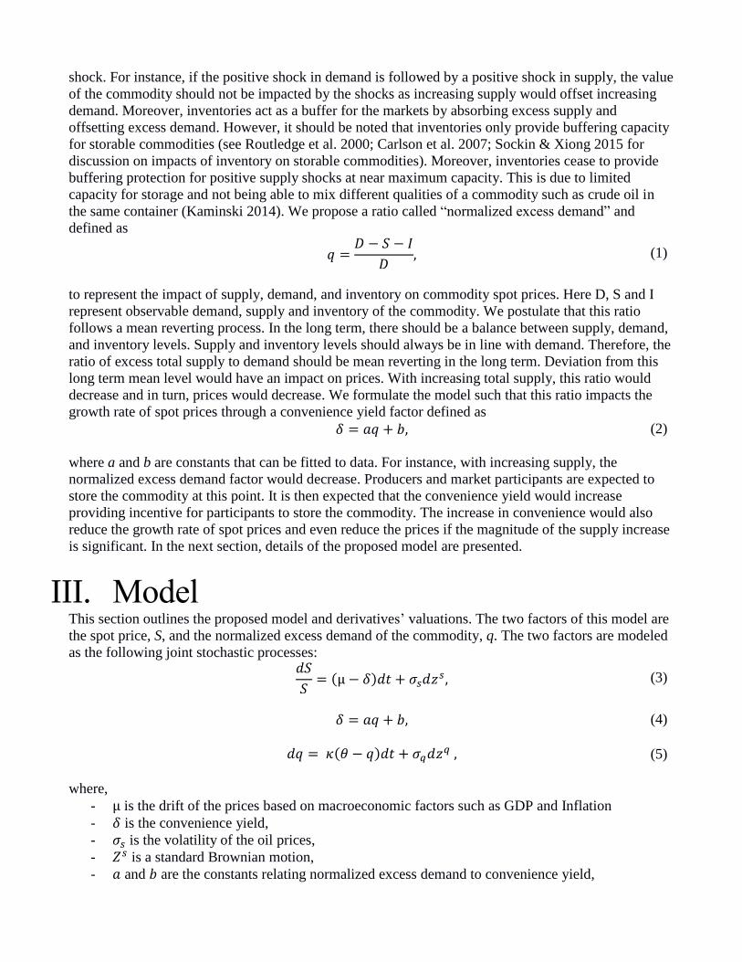
IV. Data In this section, we apply the proposed model to monthly oil market data from December 1995 to

February 2016. We use WTI futures for oil prices. WTI futures are available every month of the year

trading on the NYMEX. We select five futures contracts for calibration of the model, the 1st, 3rd, 6th,

9th, and 12th nearby contracts. These specific contracts are selected such that data corresponding to next

4 quarters are included in the model as well as representing some of the most highly liquid contracts.

Figure 1 represents the WTI futures data used for calibration.

Figure 1 Monthly WTI Futures data for 1996-2016

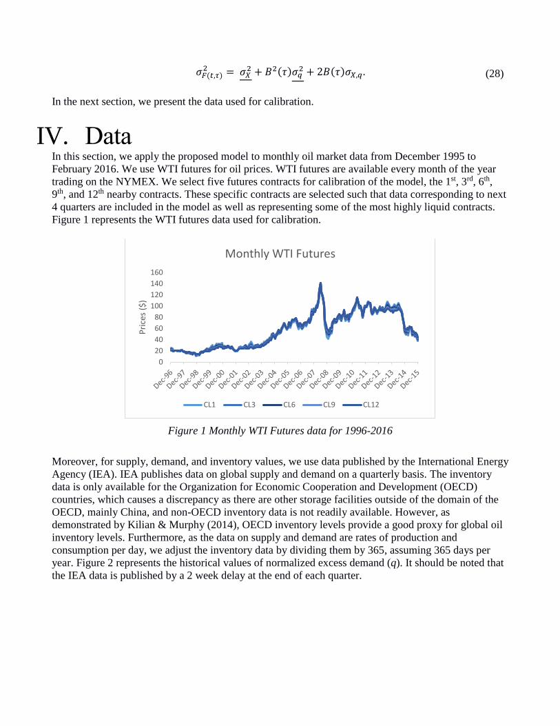
Moreover, for supply, demand, and inventory values, we use data published by the International Energy

Agency (IEA). IEA publishes data on global supply and demand on a quarterly basis. The inventory

data is only available for the Organization for Economic Cooperation and Development (OECD)

countries, which causes a discrepancy as there are other storage facilities outside of the domain of the

OECD, mainly China, and non-OECD inventory data is not readily available. However, as

demonstrated by Kilian & Murphy (2014), OECD inventory levels provide a good proxy for global oil

inventory levels. Furthermore, as the data on supply and demand are rates of production and

consumption per day, we adjust the inventory data by dividing them by 365, assuming 365 days per

year. Figure 2 represents the historical values of normalized excess demand (q). It should be noted that

the IEA data is published by a 2 week delay at the end of each quarter.

0

20

40

60

80

100

120

140

160

Pri

ces

($)

Monthly WTI Futures

CL1 CL3 CL6 CL9 CL12

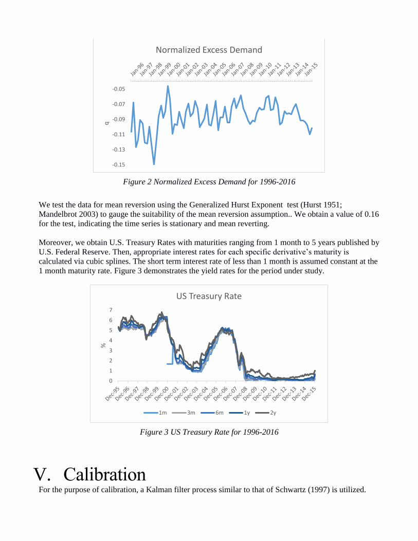
Figure 2 Normalized Excess Demand for 1996-2016

We test the data for mean reversion using the Generalized Hurst Exponent test (Hurst 1951;

Mandelbrot 2003) to gauge the suitability of the mean reversion assumption.. We obtain a value of 0.16

for the test, indicating the time series is stationary and mean reverting.

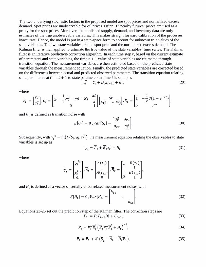
Moreover, we obtain U.S. Treasury Rates with maturities ranging from 1 month to 5 years published by

U.S. Federal Reserve. Then, appropriate interest rates for each specific derivative’s maturity is

calculated via cubic splines. The short term interest rate of less than 1 month is assumed constant at the

1 month maturity rate. Figure 3 demonstrates the yield rates for the period under study.

Figure 3 US Treasury Rate for 1996-2016

V. Calibration For the purpose of calibration, a Kalman filter process similar to that of Schwartz (1997) is utilized.

-0.15

-0.13

-0.11

-0.09

-0.07

-0.05

q

Normalized Excess Demand

0

1

2

3

4

5

6

7

%

US Treasury Rate

1m 3m 6m 1y 2y

The two underlying stochastic factors in the proposed model are spot prices and normalized excess

demand. Spot prices are unobservable for oil prices. Often, 1st nearby futures’ prices are used as a

proxy for the spot prices. Moreover, the published supply, demand, and inventory data are only

estimates of the true unobservable variables. This makes straight forward calibration of the processes

inaccurate. Hence, the model is put in a state-space form to account for unknown true values of the

state variables. The two state variables are the spot price and the normalized excess demand. The

Kalman filter is then applied to estimate the true value of the state variables’ time series. The Kalman

filter is an iterative prediction-correction algorithm. In each time step 𝑡, based on the current estimate

of parameters and state variables, the time 𝑡 + 1 value of state variables are estimated through

transition equation. The measurement variables are then estimated based on the predicted state

variables through the measurement equation. Finally, the predicted state variables are corrected based

on the differences between actual and predicted observed parameters. The transition equation relating

state parameters at time 𝑡 + 1 to state parameters at time 𝑡 is set up as

𝑥𝑡−

= 𝐶𝑡 + 𝐷𝑡𝑥𝑡−Δ𝑡 + 𝐺𝑡, (29)

where

𝑥𝑡

−= [

𝑋𝑡−

𝑞𝑡− ] , 𝐶𝑡 = [(𝜇 −

1

2𝜎𝑠

2 − 𝑎𝜃 − 𝑏)𝑎𝜃

𝜅0 1

] [Δ𝑡

𝜃(1 − 𝑒−𝜅𝑡)] , 𝐷𝑡 = [

1 −𝑎

𝜅𝜃(1 − 𝑒−𝜅𝑡)

0 𝑒−𝜅𝑡],

and 𝐺𝑡 is defined as transition noise with

𝐸[𝐺𝑡] = 0 , 𝑉𝑎𝑟[𝐺𝑡] = [

𝜎𝑋2 𝜎𝑋𝑞

𝜎𝑋𝑞 𝜎𝑞2 ]. (30)

Subsequently, with 𝑦𝑡𝜏𝑖 = ln(𝐹(𝑆𝑡, 𝑞𝑡, 𝜏𝑖)), the measurement equation relating the observables to state

variables is set up as

𝑦𝑡

= 𝐴𝑡 + 𝐵𝑡𝑥𝑡−

+ 𝐻𝑡 , (31)

where

𝑦𝑡

= [

𝑦𝑡𝜏1

⋮𝑦𝑡

𝜏12

𝑞𝑡

] , 𝐴𝑡 = [

𝐴(𝜏1)⋮

𝐴(𝜏12)0

] , 𝐵𝑡 = [

1⋮10

𝐵(𝜏1)⋮

𝐵(𝜏12)1

],

and 𝐻𝑡 is defined as a vector of serially uncorrelated measurement noises with

𝐸[𝐻𝑡] = 0 , 𝑉𝑎𝑟[𝐻𝑡] = [ℎ11

⋱ℎ66

]. (32)

Equations 23-25 set out the prediction step of the Kalman filter. The correction steps are

𝑃𝑡− = 𝐷𝑡𝑃𝑡−1𝐷𝑡

′ + 𝐺𝑡−1, (33)

𝐾𝑡 = 𝑃𝑡

−𝐵𝑡

′(𝐵𝑡𝑃𝑡

−𝐵𝑡

′+ 𝐻𝑡)

−1

, (34)

𝑥𝑡 = 𝑥𝑡−

+ 𝐾𝑡(𝑦𝑡

− 𝐴𝑡 − 𝐵𝑡𝑥𝑡−

), (35)

𝑃𝑡 = (𝐼 − 𝐾𝑡𝐴𝑡)𝑃𝑡−. (36)

The negative log-likelihood function is then derived as

1

2∑ log(𝑑𝑒𝑡(𝑉𝑡)) + 𝑒𝑡

−𝑉𝑡−1𝑒𝑡

𝑎𝑙𝑙 𝑡

, (37)

where

𝑉𝑡 = 𝐵𝑡𝑃𝑡

−𝐵𝑡

′+ 𝐻𝑡 , 𝑒𝑡 = 𝑦

𝑡− 𝐴𝑡 − 𝐵𝑡𝑥𝑡

−. (38)

Finally, this iterative system is passed to an optimization engine to maximize the likelihood function

over the underlying parameters. Lastly, the maximum likelihood estimate of the parameters, the

standard error of the parameters, and the optimal estimates of the state variables are obtained.

VI. Results The calibration process is currently in progress and the results will be presented at the conference.

VII. Conclusion Our preliminary analysis shows the importance of announcements regarding supply, demand, and

changes in inventory for the oil market. The impact of normalized excess demand is directly observable

on the market prices of crude oil. Observable normalized excess demand provides a promising channel

for quantifying the convenience yield and calibrating the underlying mean reverting process. Final

conclusions regarding the exact nature of relationship between normalized excess demand and crude oil

prices will be presented at the conference.

VIII. Appendix A This appendix represents the derivation for the join distribution of log-price and normalized excess

demand. Log-price and normalized excess demand follow a bivariate normal distribution.

Joint stochastic process for log-price and normalized excess demand can be expressed as

𝑑𝑋 = (𝜇 − 𝑎𝑞𝑡 − 𝑏 −

𝜎𝑠2

2) 𝑑𝑡 + 𝜎𝑠√1 − 𝜌2𝑑𝑧𝑠 + 𝜎𝑠𝜌𝑑𝑧𝑞 , (39)

𝑑𝑞 = [𝜅(𝜃 − 𝑞) − 𝜆]𝑑𝑡 + 𝜎𝑞𝑑𝑧𝑞 , (40)

where processes 𝑧𝑠and 𝑧𝑞are independent standard Brownian motions.

Solution to normalized excess demand can be obtained as a general Ornstein-Uhlenbeck process

𝑞𝑡 = 𝑒−𝜅𝑡𝑞0 + 𝜃(1 − 𝑒−𝜅𝑡) + 𝜎𝑞𝑒−𝜅𝑡 ∫ 𝑒𝜅𝑢𝑑𝑧𝑢

𝑞 .𝑡

0

(41)

Replacing 𝑞𝑡 in equation (39) with the solution (41) we obtain

𝑋𝑡 = 𝑋0 + (𝜇 − 𝑏 −

1

2𝜎𝑠

2) 𝑡 − ∫ 𝑎𝑞𝑢𝑑𝑢𝑡

0

+ ∫ 𝜎𝑠√1 − 𝜌2𝑑𝑧𝑢𝑠

𝑡

0

+ ∫ 𝜎𝑠𝜌𝑑𝑧𝑢𝑞

𝑡

0

, (42)

where

∫ 𝑎𝑞𝑢𝑑𝑢

𝑡

0

= ∫ 𝑎𝑒−𝜅𝑢𝑞0𝑑𝑢𝑡

0

+ ∫ 𝑎𝜃(1 − 𝑒−𝜅𝑢)𝑑𝑢𝑡

0

+ ∫ 𝑎𝜎𝑞𝑒−𝜅𝑢 (∫ 𝑒𝜅𝑤𝑑𝑧𝑤𝑞

𝑢

0

) 𝑑𝑢𝑡

0

. (43)

Applying Fubini’s theorem, the order of integration in last part of equation (21) can be changed as

∫ 𝑎𝜎𝑞𝑒−𝜅𝑢 (∫ 𝑒𝜅𝑤𝑑𝑧𝑤

𝑞𝑢

0

) 𝑑𝑢𝑡

0

= 𝑎𝜎𝑞 ∫ (∫ 𝑒−𝜅𝑢𝑒𝜅𝑤𝑑𝑢𝑡

𝑤

) 𝑑𝑧𝑤𝑞

𝑡

0

= 𝑎𝜎𝑞 ∫1

𝜅(1 − 𝑒−𝜅(𝑡−𝑤))𝑑𝑧𝑤

𝑞𝑡

0

.

(44)

Simplifying equation (21) yields

∫ 𝑎𝑞𝑢𝑑𝑢

𝑡

0

=𝑎𝑞0

𝜅(1 − 𝑒−𝜅𝑡) −

𝑎𝜃

𝜅(1 − 𝜅𝑡 − 𝑒−𝜅𝑡) + 𝑎𝜎𝑞 ∫

1

𝜅(1 − 𝑒−𝜅(𝑡−𝑤))𝑑𝑧𝑤

𝑞𝑡

0

. (45)

The spot process is then expressed as

𝑋𝑡 = 𝑋0 + (𝜇 − 𝑏 −

1

2𝜎𝑠

2 − 𝑎𝜃) 𝑡 −𝑎

𝜅(𝑞0 − 𝜃)(1 − 𝑒−𝜅𝑡) + ∫ 𝜎𝑠√1 − 𝜌2𝑑𝑧𝑢

𝑠𝑡

0

+ ∫ (𝜎𝑠𝜌 −𝑎𝜎𝑞

𝜅(1 − 𝑒−𝜅(𝑡−𝑢))𝑑𝑧𝑢

𝑞)𝑡

0

.

(46)

The following moments are then obtained for the joint distribution of log-spot price and excess demand

𝐸[𝑋𝑡] = 𝜇𝑋 = 𝑋0 + (𝜇 −

1

2𝜎𝑠

2 − 𝑎𝜃 − 𝑏) 𝑡 −𝑎

𝜅(𝑞0 − 𝜃)(1 − 𝑒−𝜅𝑡), (47)

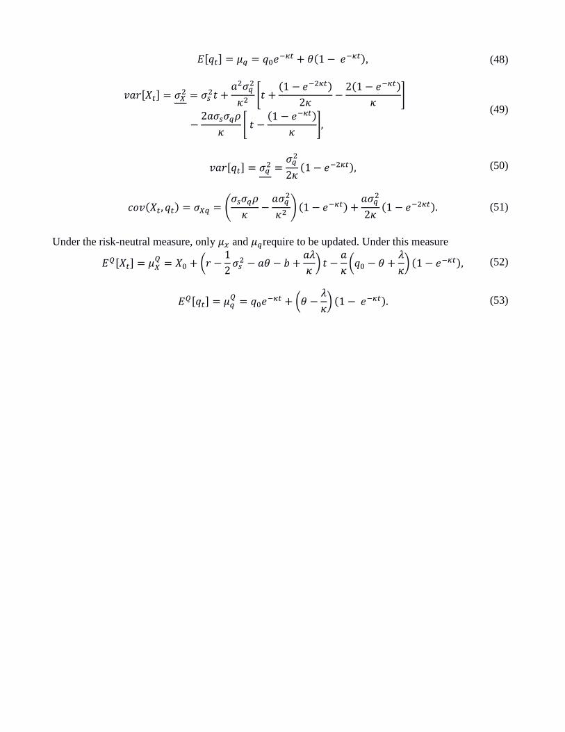
𝐸[𝑞𝑡] = 𝜇𝑞 = 𝑞0𝑒−𝜅𝑡 + 𝜃(1 − 𝑒−𝜅𝑡), (48)

𝑣𝑎𝑟[𝑋𝑡] = 𝜎𝑋

2 = 𝜎𝑠2𝑡 +

𝑎2𝜎𝑞2

𝜅2[𝑡 +

(1 − 𝑒−2𝜅𝑡)

2𝜅−

2(1 − 𝑒−𝜅𝑡)

𝜅]

−2𝑎𝜎𝑠𝜎𝑞𝜌

𝜅[ 𝑡 −

(1 − 𝑒−𝜅𝑡)

𝜅],

(49)

𝑣𝑎𝑟[𝑞𝑡] = 𝜎𝑞

2 =𝜎𝑞

2

2𝜅(1 − 𝑒−2𝜅𝑡), (50)

𝑐𝑜𝑣(𝑋𝑡, 𝑞𝑡) = 𝜎𝑋𝑞 = (

𝜎𝑠𝜎𝑞𝜌

𝜅−

𝑎𝜎𝑞2

𝜅2) (1 − 𝑒−𝜅𝑡) +

𝑎𝜎𝑞2

2𝜅(1 − 𝑒−2𝜅𝑡). (51)

Under the risk-neutral measure, only 𝜇𝑥 and 𝜇𝑞require to be updated. Under this measure

𝐸𝑄[𝑋𝑡] = 𝜇𝑋

𝑄 = 𝑋0 + (𝑟 −1

2𝜎𝑠

2 − 𝑎𝜃 − 𝑏 +𝑎𝜆

𝜅) 𝑡 −

𝑎

𝜅(𝑞0 − 𝜃 +

𝜆

𝜅) (1 − 𝑒−𝜅𝑡), (52)

𝐸𝑄[𝑞𝑡] = 𝜇𝑞

𝑄 = 𝑞0𝑒−𝜅𝑡 + (𝜃 −𝜆

𝜅) (1 − 𝑒−𝜅𝑡). (53)

References Bastian-Pinto, C., Brandão, L. & Hahn, W.J., 2009. Flexibility as a source of value in the production of

alternative fuels : The ethanol case. Energy Economics, 31(3), pp.411–422. Available at:

http://dx.doi.org/10.1016/j.eneco.2009.02.004.

Baumeister, C. & Kilian, L., 2016. Real-Time Forecasts of the Real Price of Oil Real-Time Forecasts

of the Real Price of Oil. Journal of Business & Economic Statistics, 30(2), pp.326–336.

BIS, 2015. Semiannual OTC derivatives statistics,

Brandão, L.E.T., Penedo, G.M. & Bastian-Pinto, C., 2013. The value of switching inputs in a biodiesel

production plant. The European Journal of Finance, 2013, 19(7-8), pp.674–688.

Bu, H., 2014. Effect of inventory announcements on crude oil price volatility. Energy Economics, 46,

pp.485–494. Available at: http://dx.doi.org/10.1016/j.eneco.2014.05.015.

Carlson, M., Khokher, Z. & Titman, S., 2007. Resource Price Dynamics. The Journal of Finance,

LXII(4), pp.1663–1703.

Casassus, J. & Collin-Dufresne, P., 2005. Stochastic Convenience Yield Implied from Commodity

Futures and Interest Rates. The Journal of Finance, 60(5), pp.2283–2331.

Chen, S. & Insley, M., 2012. Regime switching in stochastic models of commodity prices: An

application to an optimal tree harvesting problem. Journal of Economic Dynamics and Control,

36(2), pp.201–219. Available at: http://dx.doi.org/10.1016/j.jedc.2011.08.010.

Chiang, I.E., Hughen, W.K. & Sagi, J.S., 2015. Estimating Oil Risk Factors Using Information from

Equity and Derivatives Markets. The Journal of Finance, LXX(2), pp.769–804.

Cuñado, J. & Gracia, F.P. de, 2003. Do oil price shocks matter? Evidence for some European countries.

Energy Economics, 25(2), pp.137–154. Available at:

http://www.sciencedirect.com/science/article/pii/S0140988302000993.

Erb, C.B. & Harvey, C.R., 2006. The Strategic and Tactical Value of Commodity Futures. Financial

Analysts Journal, 62(2), pp.69–97.

Geman, H., 2005. Commodities and Commodity Derivatives: Modeling and Pricing for Agriculturals,

Metals and Energy, Chichester, West Sussex, England: Wiley & Sons, Ltd.

Gibson, R. & Schwartz, E.S., 1990. Stochastic Convenience Yield and the Pricing of Oil Contingent

Claims. The Journal of Finance, 45(3), pp.959–976. Available at:

http://onlinelibrary.wiley.com/doi/10.1111/j.1540-6261.1990.tb05114.x/abstract.

Gorton, G. & Rouwenhorst, K.G., 2006. Facts and Fantasies about Commodity Futures. Financial

Analysts Journal, 62(2), pp.47–68. Available at: http://www.jstor.org/stable/4480744.

Greer, R.J., 2000. The Nature of Commodity Index Returns. THE JOURNAL OF ALTERNATIVE

INVESTMENTS, 3, pp.45–53.

Güntner, J.H.F., 2014. How do oil producers respond to oil demand shocks ? Energy Economics, 44,

pp.1–13. Available at: http://dx.doi.org/10.1016/j.eneco.2014.03.012.

Hamilton, J.D., 2011. Nonlinearities and the Macroeconomic Effects of Oil Prices. Macroeconomic

Dynamics, 15(Supplement 3), pp.364–378.

Hamilton, J.D., 2008. “Oil and the Macroeconomy.” In S. N. Durlauf & L. E. Blume, eds. In The New

Palgrave Dictionary of Economics. Palgrave Macmillan.

Hikspoors, S. & Jaimungal, S., 2008. Asymptotic Pricing of Commodity Derivatives using Stochastic

Volatility Spot Models. Applied Mathematical Finance, 15(5-6), pp.449–477.

Hurst, H.E., 1951. Long-term storage capacity of reservoirs. Transactions of American Society of Civil

Engineers, 116, pp.770–808.

Juvenal, L. & Petrella, I., 2015. SPECULATION IN THE OIL MARKET. Journal of Applied

Econometrics, 30(4), pp.621–649.

Kaminski, V., 2014. The microstructure of the North American oil market. Energy Economics, 46,

pp.S1–S10. Available at: http://dx.doi.org/10.1016/j.eneco.2014.10.017.

Kilian, L., 2014. Oil Price Shocks : Causes and Consequences. The Annual Review of Resource

Economics, 6, pp.133–154.

Kilian, L. & Lee, T.K., 2014. Quantifying the speculative component in the real price of oil: The role

of global oil inventories. Journal of International Money and Finance, 42, pp.71–87. Available at:

http://dx.doi.org/10.1016/j.jimonfin.2013.08.005.

Kilian, L. & Murphy, D.P., 2014. THE ROLE OF INVENTORIES AND SPECULATIVE TRADING

IN THE GLOBAL MARKET FOR CRUDE OIL. Journal of Applied Econometrics, 29(3),

pp.454–478.

Kobari, L., Jaimungal, S. & Lawryshyn, Y., 2014. A real options model to evaluate the effect of

environmental policies on the oil sands rate of expansion. Energy Economics, 45, pp.155–165.

Available at: http://dx.doi.org/10.1016/j.eneco.2014.06.010.

Lai, A.N. & Mellios, C., 2016. Valuation of commodity derivatives with an unobservable convenience

yield. Computers and Operations Research, 66, pp.402–414. Available at:

http://dx.doi.org/10.1016/j.cor.2015.03.007.

Liu, P. & Tang, K., 2011. The stochastic behavior of commodity prices with heteroskedasticity in the

convenience yield. Journal of Empirical Finance, 18(2), pp.211–224. Available at:

http://dx.doi.org/10.1016/j.jempfin.2010.12.003.

Mandelbrot, B.B., 2003. HEAVY TAILS IN FINANCE FOR INDEPENDENT OR MULTIFRACTAL

PRICE INCREMENTS. In S.T. Rachev, ed. Handbook of Heavy Tailed Distributions in Finance.

Elsevier Science B.V.

Mirantes, A.G., Población, J. & Serna, G., 2013. The stochastic seasonal behavior of energy

commodity convenience yields. Energy Economics, 40, pp.155–166. Available at:

http://dx.doi.org/10.1016/j.eneco.2013.06.011.

Morana, C., 2013. The Oil Price-Macroeconomy Relationship Since the Mid-1980s: A Global

Perspective. The Energy Journal, 34(3), pp.153–189.

Routledge, B.R., Seppi, D.J. & Spatt, C.S., 2000. Equilibrium Forward Curves for Commodities. The

Journal of Finance, LV(3), pp.1297–1338.

Schwartz, E.S., 1997. The Stochastic Behavior of Commodity Prices : Implications for Valuation and

Hedging. The Journal of Finance, LII(3), pp.923–973.

Sockin, M. & Xiong, W., 2015. Informational Frictions and Commodity Markets. The Journal of

Finance, LXX(5), pp.2063–2098.

Stefanski, R., 2014. Structural transformation and the oil price. Review of Economic Dynamics, 17(3),

pp.484–504. Available at: http://dx.doi.org/10.1016/j.red.2013.09.006.

Szymanowska, M. et al., 2014. An Anatomy of Commodity Futures Risk Premia. The Journal of

Finance, LXIX(1), pp.453–482.

Trolle, A.B. & Schwartz, E.S., 2009. Unspanned Stochastic Volatility and the Pricing of Commodity

Derivatives. The Review of Financial Studies, 22(11), pp.4423–4461.