Download pdf - ADAPTIVE MAXIMUM POWER POINT TRACKING ALGORITHM … · ADAPTIVE MAXIMUM POWER POINT TRACKING ALGORITHM FOR MULTI-VARIABLE APPLICATIONS IN PHOTOVOLTAIC ARRAYS Andrés Julián sAAvedrA

ADAPTIVE MAXIMUM POWER POINT TRACKING ALGORITHM FOR MULTI-VARIABLE APPLICATIONS IN

PHOTOVOLTAIC ARRAYS

Andrés Julián sAAvedrA Montes*

CArlos Andrés rAMos PAJA**

luz AdriAnA treJos GrisAles***

ABSTRACT

Classical algorithms for multi-variable photovoltaic systems use fixed-size perturbations, which does not optimize the produced power in both steady-state and transient conditions. Therefore, an adaptive maximum power point tracking algorithm for photovoltaic systems is proposed in this paper to improve the power generation in both transient and steady-state conditions. The proposed algorithm only uses a single pair of current/voltage sensors to reach the global maximum available power, which contrast with the high number of sensors required by others distributed maximum power point tracking solutions. The algorithm recognizes the voltage pattern exhibited by PV system in both steady-state and transient conditions to adapt the size perturbations accordingly: in steady-state conditions reduces the perturbation size to minimize the power loses, while in transient conditions increases the perturbation size to speed-up the tracking of the new operating point. Finally, the adaptive multi-variable perturb and observe algorithm is validated by means of simulation using detailed models.

KEYWORDS: Photovoltaic Generation; Adaptive Algorithm; Maximum Power Point; Efficiency.

ALGORITMO ADAPTATIVO PARA SEGUIMIENTO DEL PUNTO DE MÁXIMA POTENCIA EN APLICACIONES MULTI-VARIABLES DE

CAMPOS FOTOVOLTAICOS

RESUMEN

Los algoritmos clásicos para sistemas fotovoltaicos multi-variables usan perturbaciones con amplitud fija, lo cual no optimiza la potencia producida en condiciones estacionarias y transitorias. Por tanto, en este artículo se propone un algoritmo adaptativo para el seguimiento del punto de máxima potencia, el cual incrementa la potencia generada en condiciones estacionarias y transitorias. El algoritmo requiere un único par de sensores de corriente/voltaje para alcanzar el punto de potencia máxima global, en contraste con el alto número de sensores requeridos por otras soluciones distribuidas

Historia del artículo:Artículo recibido: 28-V-2013 / Aprobado: 05-XI-2013Discusión abierta hasta diciembre de 2014

Autor de correspondencia: (A.J. Saavedra-Montes). Carrera 80 N. 65-223 - Facultad de Minas Bloque M8 - Oficina 113, Medellín (Colombia). Tel: 4 4255297. Correo electrónico: [email protected]

DOI: http:/dx.doi.org/10.14508/reia.2013.10.20.193-206

Revista EIA, ISSN 1794-1237/ Año X/ Volumen 10 / Número 20 / Julio-Diciembre 2013 /pp. 193-206Publicación semestral de carácter técnico-científico / Escuela de Ingeniería de Antioquia —EIA—, Medellín (Colombia)

* Ingeniero electricista, Magíster en Sistemas de Generación de Energía Eléctrica, Doctor en Ingeniería Eléctrica, Universidad del Valle. Profesor Asociado Universidad Nacional de Colombia, sede Medellín. Medellín (Colombia).

** Ingeniero electrónico, Doctor en Ingeniería Electrónica, Automática y Comunicaciones, Universidad Nacional de Colombia, sede Medellín. Profesor Asistente Universidad Nacional de Colombia, sede Medellín. Medellín (Colombia).

*** Ingenieria electricista, candidata a Doctora en Ingeniería, Universidad Nacional de Colombia, sede Medellín. Medellín (Colombia).

194

AdAptive mAximum power point trAcking Algorithm for multi-vAriAble ApplicAtions in photovoltAic ArrAys

Revista EIA Rev.EIA.Esc.Ing.Antioq / Publicación semestral Escuela de Ingeniería de Antioquia —EIA—

del seguimiento del punto de máxima potencia. El algoritmo reconoce el patrón de voltaje descrito por el sistema fotovoltaico en condiciones estacionarias y transitorias para adaptar el tamaño de las perturbaciones: es condiciones estacionarias reduce el tamaño de las perturbaciones para minimizar las pérdidas de potencia, mientras que en condiciones transitorias incrementa el tamaño de las perturbaciones para acelerar el seguimiento del nuevo punto de operación. Finalmente, el algoritmo es validado a través de simulación utilizando un modelo matemático detallado de un sistema fotovoltaico.

PALABRAS CLAVES: generación fotovoltaica; algoritmo adaptativo; punto de máxima potencia y eficiencia.

ALGORÍTMO ADAPTATIVO PARA RASTREAMENTO DO PONTO DE MÁXIMA POTÊNCIA EM APLICAÇÕES MULTI-VARIÁVEIS DE

CAMPOS FOTOVOLTAICOS

SUMÁRIO

Os algorítmos clássicos para sistemas fotovoltaicos multi-variáveis usam perturbações com amplitude fixa, o qual não otimiza a potência produzida em condições estacionárias e transitórias. Por tanto, em este artigo propõe-se um algorítmo adaptativo para o rastreamento do ponto de máxima potência, o qual incrementa a potência gerada em condições estacionárias e transitórias. O algorítmo requer um único par de sensores de corrente/voltaje para atingir o ponto de potência máxima global, em contraste com o alto número de sensores requeridos por outras soluções distribuídas do rastreamento do ponto de máxima potência. O algorítmo reconhece o padrão de voltaje descrito pelo sistema fotovoltaico em condições estacionárias e transitórias para adaptar o tamanho das perturbações: é condições estacionárias reduz o tamanho das perturbações para minimizar as perdas de potência, enquanto em condições transi-tórias incrementa o tamanho das perturbações para acelerar o rastreamento do novo ponto de operação. Finalmente, o algorítmo é validado através de simulação utilizando um modelo matemático detalhado de um sistema fotovoltaico.

PALAVRAS-CHAVE: Geração fotovoltaica; Algorítmo adaptativo; Ponto de máxima potência e eficiência.

1. INTRODUCTION

Photovoltaic (PV) power systems provide electrical power in agreement with the solar irradiance and temperature acting on the PV modules as reported by Femia, et al. (2009) and Femia, et al. (2005). Therefore, a large amount of possible operating points can occur since multiple environmental conditions can be present in different modules of the PV array as presented by Femia, et al. (2008).

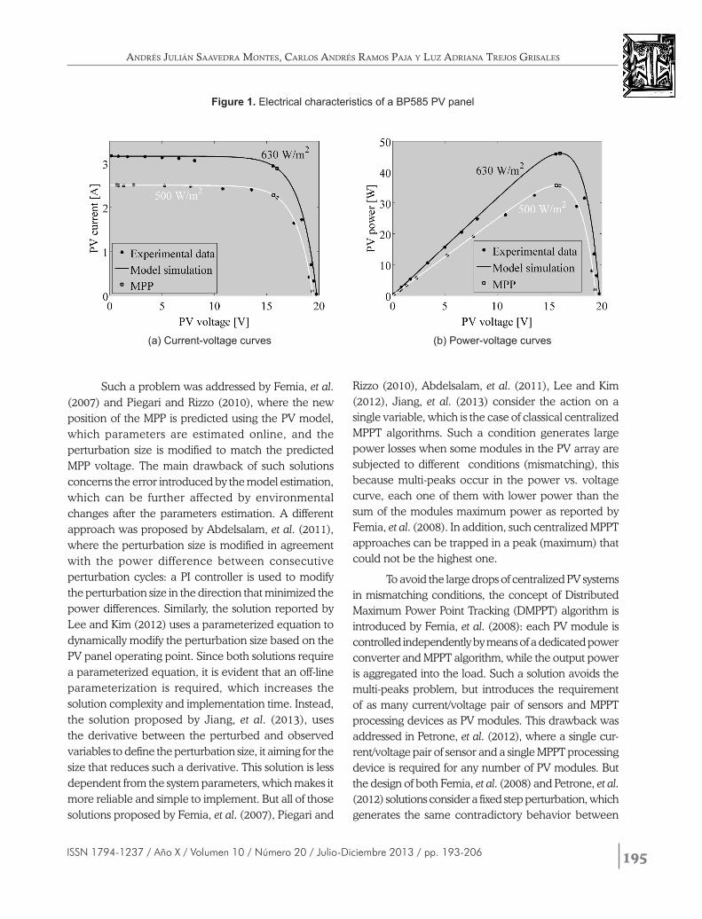
In addition, each PV module can operate in mul-tiple operation conditions as observed in figure 1, where the experimental electrical characteristics of a BP585 PV panel, composed by two PV modules, are reported for two different irradiances. Such a figure also depicts the electrical behavior simulation of the BP585 module by means of the PV model reported by Petrone and Ramos-Paja (2011). From figure 1 is evident that an optimal point exists, named Maximum Power Point (MPP), in which the

PV panel produces the maximum power available for the particular environmental conditions.

Several search algorithms, named Maximum Power Point Tracking (MPPT) algorithms, have been proposed in literature by Subudhi and Pradhan (2013) to find the MPP. Among them, the Perturb and Observe (PO) algorithm reported by Femia, et al. (2005), Femia, et al. (2009) is the most widely adopted due to its sim-plicity and satisfactory performance. Such a solution perturbs the PV voltage in the direction that increases the PV power, where classical implementations define the perturbation size to provide a trade-off between tracking speed and steady-state power losses: large perturbation sizes provide fast tracking of a new MPP, but also generate high steady-state power losses due to the large oscillation around the MPP; instead, short perturbation sizes provide small steady-state power losses, but due to the small power in the perturbed variable, the transition to a new MPP is slow, generating additional power losses.

195ISSN 1794-1237 / Año X / Volumen 10 / Número 20 / Julio-Diciembre 2013 / pp. 193-206

Such a problem was addressed by Femia, et al. (2007) and Piegari and Rizzo (2010), where the new position of the MPP is predicted using the PV model, which parameters are estimated online, and the perturbation size is modified to match the predicted MPP voltage. The main drawback of such solutions concerns the error introduced by the model estimation, which can be further affected by environmental changes after the parameters estimation. A different approach was proposed by Abdelsalam, et al. (2011), where the perturbation size is modified in agreement with the power difference between consecutive perturbation cycles: a PI controller is used to modify the perturbation size in the direction that minimized the power differences. Similarly, the solution reported by Lee and Kim (2012) uses a parameterized equation to dynamically modify the perturbation size based on the PV panel operating point. Since both solutions require a parameterized equation, it is evident that an off-line parameterization is required, which increases the solution complexity and implementation time. Instead, the solution proposed by Jiang, et al. (2013), uses the derivative between the perturbed and observed variables to define the perturbation size, it aiming for the size that reduces such a derivative. This solution is less dependent from the system parameters, which makes it more reliable and simple to implement. But all of those solutions proposed by Femia, et al. (2007), Piegari and

(a) Current-voltage curves (b) Power-voltage curves

Figure 1. Electrical characteristics of a BP585 PV panel

Rizzo (2010), Abdelsalam, et al. (2011), Lee and Kim (2012), Jiang, et al. (2013) consider the action on a single variable, which is the case of classical centralized MPPT algorithms. Such a condition generates large power losses when some modules in the PV array are subjected to different conditions (mismatching), this because multi-peaks occur in the power vs. voltage curve, each one of them with lower power than the sum of the modules maximum power as reported by Femia, et al. (2008). In addition, such centralized MPPT approaches can be trapped in a peak (maximum) that could not be the highest one.

To avoid the large drops of centralized PV systems in mismatching conditions, the concept of Distributed Maximum Power Point Tracking (DMPPT) algorithm is introduced by Femia, et al. (2008): each PV module is controlled independently by means of a dedicated power converter and MPPT algorithm, while the output power is aggregated into the load. Such a solution avoids the multi-peaks problem, but introduces the requirement of as many current/voltage pair of sensors and MPPT processing devices as PV modules. This drawback was addressed in Petrone, et al. (2012), where a single cur-rent/voltage pair of sensor and a single MPPT processing device is required for any number of PV modules. But the design of both Femia, et al. (2008) and Petrone, et al. (2012) solutions consider a fixed step perturbation, which generates the same contradictory behavior between

Andrés Julián sAAvedrA montes, cArlos Andrés rAmos pAJA y luz AdriAnA treJos grisAles

196



tracking speed and steady-state power losses present in the classical PO algorithm.

Therefore, this paper proposes a DMPPT algo-rithm with adaptive perturbation size, which is aimed at improving the power generation in both transient and steady-state conditions. The proposed solution is based on the DMPPT idea introduced by Petrone, et al. (2012), but considering an asynchronous modifica-tion of the perturbation size for all the PV modules. In addition, the proposed adaptive technique is based on the novel idea of reducing the perturbation size when the PV system is in steady-state conditions, and increas-ing it in other transient conditions. This solution does not require any model or parameters estimation, or derivative calculation, since it is based on the pattern recognition of stable PO profiles. Hence, the proposed DMPPT algorithm improves the power extraction from PV arrays, and it is more reliable and easy to implement than both classical solutions for DMPPT and adaptive algorithms.

2. ADAPTIVE PERTURBATION BASED ON PATTERN RECOGNITION

The classical PO algorithm, as many other classi-cal algorithms reported by Subudhi and Pradhan (2013), acts directly on the duty cycle D of a dc/dc converter or indirectly on the reference Vref of a closed-loop PV voltage control. The PO algorithm is designed by means of two parameters: the perturbation period Ta and the perturbation size ∆M. The former is defined to be larger than the PV system settling time, which in open loop (perturbing D) is imposed by the dc/dc converter passive elements, while in closed loop (perturbing Vref) is imposed by the control system Femia, et al. (2009). In both cases, the time interval Ta between the signal perturbation and the analysis of its effect must be larger, or at least equal, to the system settling-time, otherwise the MPPT algorithm will observe a transient power dif-ferent from the steady-state value, and the subsequent decision will be based on incorrect information leading to a wrong operation as described by Femia, et al. (2009) and Femia, et al. (2005). Despite Jiang, et al. (2013) proposes to dynamically modify Ta, such a feature does not impact the power losses in a significant way: if ∆M is large enough, the tracking of a new MPP is fast, which

reduces the transient power losses; while if ∆M is small enough, the steady-state oscillation around the MPP is also small, which reduces the steady-state power losses. Therefore, as adopted in Femia, et al. (2007), Piegari and Rizzo (2010), Abdelsalam, et al. (2011), Lee and Kim (2012), the modification of ∆M with a fixed Ta is enough to implement an adaptive MPPT algorithm.

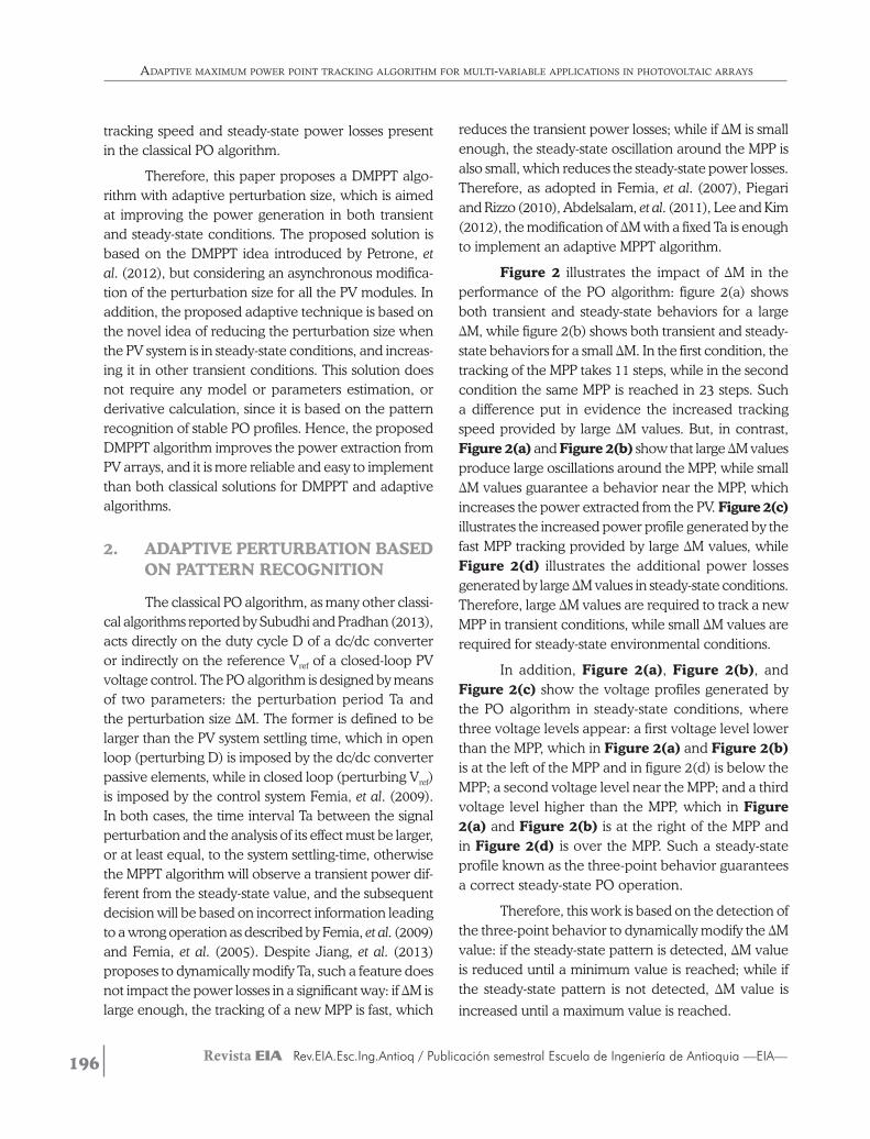
Figure 2 illustrates the impact of ∆M in the performance of the PO algorithm: figure 2(a) shows both transient and steady-state behaviors for a large ∆M, while figure 2(b) shows both transient and steady-state behaviors for a small ∆M. In the first condition, the tracking of the MPP takes 11 steps, while in the second condition the same MPP is reached in 23 steps. Such a difference put in evidence the increased tracking speed provided by large ∆M values. But, in contrast, Figure 2(a) and Figure 2(b) show that large ∆M values produce large oscillations around the MPP, while small ∆M values guarantee a behavior near the MPP, which increases the power extracted from the PV. Figure 2(c) illustrates the increased power profile generated by the fast MPP tracking provided by large ∆M values, while Figure 2(d) illustrates the additional power losses generated by large ∆M values in steady-state conditions. Therefore, large ∆M values are required to track a new MPP in transient conditions, while small ∆M values are required for steady-state environmental conditions.

In addition, Figure 2(a), Figure 2(b), and Figure 2(c) show the voltage profiles generated by the PO algorithm in steady-state conditions, where three voltage levels appear: a first voltage level lower than the MPP, which in Figure 2(a) and Figure 2(b) is at the left of the MPP and in figure 2(d) is below the MPP; a second voltage level near the MPP; and a third voltage level higher than the MPP, which in Figure 2(a) and Figure 2(b) is at the right of the MPP and in Figure 2(d) is over the MPP. Such a steady-state profile known as the three-point behavior guarantees a correct steady-state PO operation.

Therefore, this work is based on the detection of the three-point behavior to dynamically modify the ∆M value: if the steady-state pattern is detected, ∆M value is reduced until a minimum value is reached; while if the steady-state pattern is not detected, ∆M value is

increased until a maximum value is reached.


2.1 Pattern Recognition of the Three-Point Behavior

To detect the steady-state operation of the PV sys-

tem, the PO three-point behavior (TPB) on the manipu-

lated variable, duty-cycle or reference voltage, must be

recognized. In the proposed solution, such a procedure is

performed by the TPB detector, which inspects the output

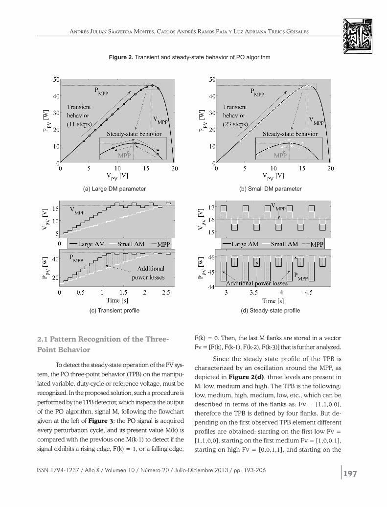
of the PO algorithm, signal M, following the flowchart

given at the left of Figure 3: the PO signal is acquired

every perturbation cycle, and its present value M(k) is

compared with the previous one M(k-1) to detect if the

signal exhibits a rising edge, F(k) = 1, or a falling edge,

F(k) = 0. Then, the last M flanks are stored in a vector Fv = [F(k), F(k-1), F(k-2), F(k-3)] that is further analyzed.

Since the steady state profile of the TPB is characterized by an oscillation around the MPP, as depicted in Figure 2(d), three levels are present in M: low, medium and high. The TPB is the following: low, medium, high, medium, low, etc., which can be described in terms of the flanks as: Fv = [1,1,0,0], therefore the TPB is defined by four flanks. But de-pending on the first observed TPB element different profiles are obtained: starting on the first low Fv = [1,1,0,0], starting on the first medium Fv = [1,0,0,1], starting on high Fv = [0,0,1,1], and starting on the

(a) Large DM parameter (b) Small DM parameter

(c) Transient profile (d) Steady-state profile

Figure 2. Transient and steady-state behavior of PO algorithm


198



second medium Fv = [0,1,1,0]. The last example is

illustrated in the right side of Figure 3, where Fv is

constructed with the flanks that occur after the sec-

ond medium level of M. Moreover, from the previous

analysis it is noted that the TPB, expressed in terms

of flanks, exhibits two consecutive flanks of the same

value, i.e. [1,1] or [0,0]. Therefore, as described in

the flowchart of figure 3, the PO is in steady state

(SS = 1) if Fv has two consecutive elements with

the same value, i.e. [1,1] or [0,0], otherwise the PO

is in transient condition (SS = 0).

Figure 3. TPB detector flowchart

Figure 4. DM modifier flowchart

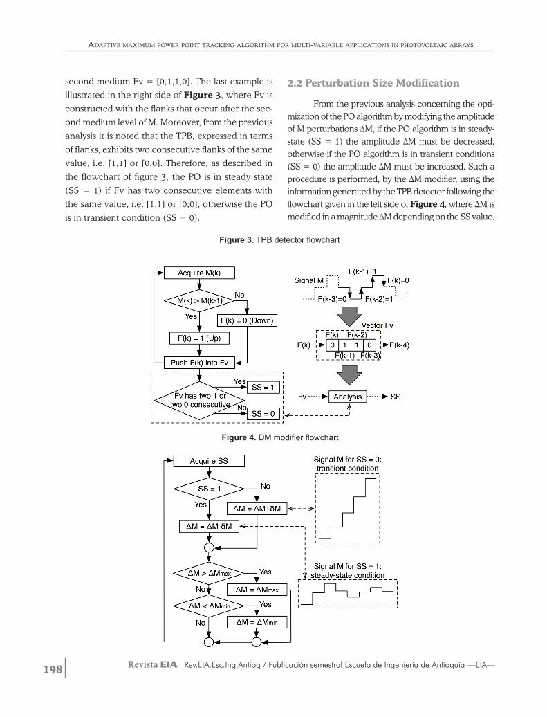
2.2 Perturbation Size Modification

From the previous analysis concerning the opti-mization of the PO algorithm by modifying the amplitude of M perturbations ∆M, if the PO algorithm is in steady-state (SS = 1) the amplitude ∆M must be decreased, otherwise if the PO algorithm is in transient conditions (SS = 0) the amplitude ∆M must be increased. Such a procedure is performed, by the ∆M modifier, using the information generated by the TPB detector following the flowchart given in the left side of Figure 4, where ∆M is modified in a magnitude ∆M depending on the SS value.


Moreover, the maximum and minimum values of ∆M are constrained to ∆Mmax and ∆Mmin, respectively. The right side of figure 4 illustrates the transient and steady-state profiles of the PO algorithm under the action of the ∆M modifier: signal M is increased to track the MPP, while M is decreased around the MPP to reduce the power losses due to the PO oscillation.

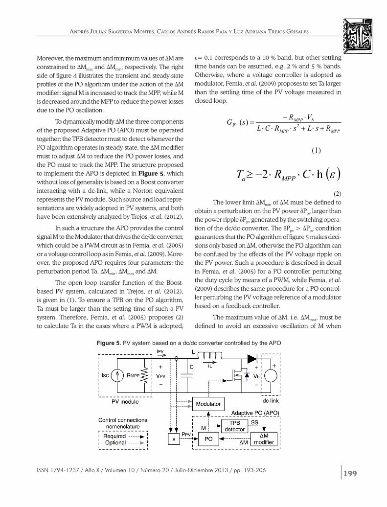
To dynamically modify ∆M the three components of the proposed Adaptive PO (APO) must be operated together: the TPB detector must to detect whenever the PO algorithm operates in steady-state, the ∆M modifier must to adjust ∆M to reduce the PO power losses, and the PO must to track the MPP. The structure proposed to implement the APO is depicted in Figure 5, which without loss of generality is based on a Boost converter interacting with a dc-link, while a Norton equivalent represents the PV module. Such source and load repre-sentations are widely adopted in PV systems, and both have been extensively analyzed by Trejos, et al. (2012).

In such a structure the APO provides the control signal M to the Modulator that drives the dc/dc converter, which could be a PWM circuit as in Femia, et al. (2005) or a voltage control loop as in Femia, et al. (2009). More-over, the proposed APO requires four parameters: the perturbation period Ta, ∆Mmin, ∆Mmax and ∆M.

The open loop transfer function of the Boost-based PV system, calculated in Trejos, et al. (2012), is given in (1). To ensure a TPB on the PO algorithm, Ta must be larger than the setting time of such a PV system. Therefore, Femia, et al. (2005) proposes (2) to calculate Ta in the cases where a PWM is adopted,

ε= 0,1 corresponds to a 10 % band, but other settling time bands can be assumed, e.g. 2 % and 5 % bands. Otherwise, where a voltage controller is adopted as modulator, Femia, et al. (2009) proposes to set Ta larger than the settling time of the PV voltage measured in closed loop.

MPPMPP

bMPPPV RsLsRCL

VRsG+⋅+⋅⋅⋅

⋅−= 2)(

(1)

( )εln2 ⋅⋅⋅−≥ CRT MPPa

(2)The lower limit ∆Mmin of ∆M must be defined to

obtain a perturbation on the PV power δPpv larger than the power ripple δPpv generated by the switching opera-tion of the dc/dc converter. The δPpv > ∆Ppv condition guarantees that the PO algorithm of figure 5 makes deci-sions only based on ∆M, otherwise the PO algorithm can be confused by the effects of the PV voltage ripple on the PV power. Such a procedure is described in detail in Femia, et al. (2005) for a PO controller perturbing the duty cycle by means of a PWM, while Femia, et al. (2009) describes the same procedure for a PO control-ler perturbing the PV voltage reference of a modulator based on a feedback controller.

The maximum value of ∆M, i.e. ∆Mmax, must be defined to avoid an excessive oscillation of M when

Figure 5. PV system based on a dc/dc converter controlled by the APO


200



the algorithm reaches the MPP. This work considers a ∆Mmax = 50·∆Mmin to illustrate the solution behavior with a large excursion of ∆M, but any other value can be adopted. In a similar way, ∆M must be defined in a trade off between tracking speed and converge to the optimal ∆M: large ∆M provides a fast tracking of a new MPP, but such large ∆M value avoids a fine tuning of the optimal ∆M value. Instead, small ∆M allows to accurately detecting the best ∆M value, but in contrast the tracking of the MPP is slow due to the small changes on ∆M. This work considers a ∆M = ∆Mmin/2 to provide trade off between tracking speed and converge to the optimal ∆M, however any other value can be adopted.

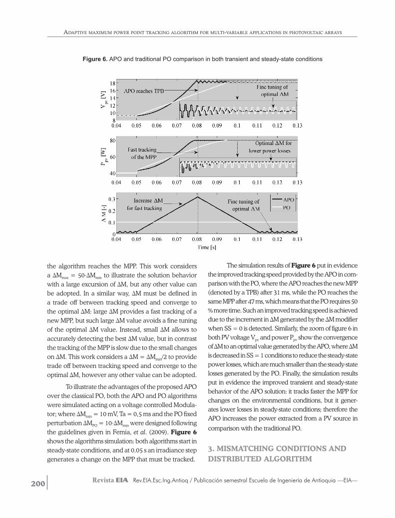
To illustrate the advantages of the proposed APO over the classical PO, both the APO and PO algorithms were simulated acting on a voltage controlled Modula-tor; where ∆Mmin = 10 mV, Ta = 0,5 ms and the PO fixed perturbation ∆MPO = 10·∆Mmin were designed following the guidelines given in Femia, et al. (2009). Figure 6 shows the algorithms simulation: both algorithms start in steady-state conditions, and at 0.05 s an irradiance step generates a change on the MPP that must be tracked.

The simulation results of Figure 6 put in evidence the improved tracking speed provided by the APO in com-parison with the PO, where the APO reaches the new MPP (denoted by a TPB) after 31 ms, while the PO reaches the same MPP after 47 ms, which means that the PO requires 50 % more time. Such an improved tracking speed is achieved due to the increment in ∆M generated by the ∆M modifier when SS = 0 is detected. Similarly, the zoom of figure 6 in both PV voltage Vpv and power Ppv show the convergence of ∆M to an optimal value generated by the APO, where ∆M is decreased in SS = 1 conditions to reduce the steady-state power losses, which are much smaller than the steady-state losses generated by the PO. Finally, the simulation results put in evidence the improved transient and steady-state behavior of the APO solution: it tracks faster the MPP for changes on the environmental conditions, but it gener-ates lower losses in steady-state conditions; therefore the APO increases the power extracted from a PV source in

comparison with the traditional PO.

3. MISMATCHING CONDITIONS AND DISTRIBUTED ALGORITHM

Figure 6. APO and traditional PO comparison in both transient and steady-state conditions


The previous APO algorithm acts on a single vari-

able, thus it is subjected to the same problems of the PO

acting on a PV array in mismatching conditions, which

could be trapped in a suboptimal maximum power or

Local MPP (LMPP) instead of the global MPP (GMPP).

But it must be point out that all the LMPP in an array,

including the GMPP, exhibit an array power lower than

the Maximum Available PV (MAPV) power, which cor-

responds to the sum of all the MPP powers available in

each PV module.

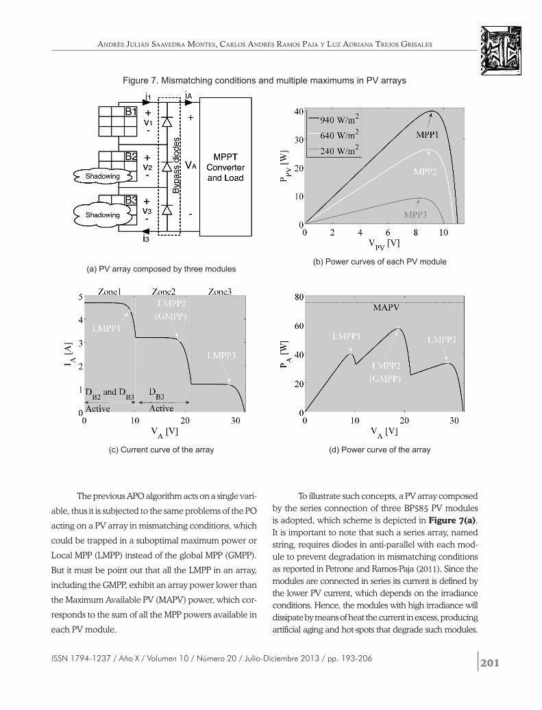
To illustrate such concepts, a PV array composed by the series connection of three BP585 PV modules is adopted, which scheme is depicted in Figure 7(a). It is important to note that such a series array, named string, requires diodes in anti-parallel with each mod-ule to prevent degradation in mismatching conditions as reported in Petrone and Ramos-Paja (2011). Since the modules are connected in series its current is defined by the lower PV current, which depends on the irradiance conditions. Hence, the modules with high irradiance will dissipate by means of heat the current in excess, producing artificial aging and hot-spots that degrade such modules.

(a) PV array composed by three modules(b) Power curves of each PV module

(c) Current curve of the array (d) Power curve of the array

Figure 7. Mismatching conditions and multiple maximums in PV arrays


202



To prevent those undesired conditions, the anti-parallel diodes, named bypass diodes, provide an alternative path to the difference between the larger current of the modules with higher irradiance and the smaller current of the mod-ules with lower irradiance. In such a new condition, the string current is defined by the higher PV current, where the activation of a bypass diode imposes a short-circuit condition to the associated PV module, imposing a null power production to such a module.

The scheme Figure 7(a) also includes a MPPT controller and a dc/dc converter that interacts with the load, which consists in a grid-connected inverter. Since such a MPPT technique perturbs the array voltage only, it represents a centralized solution or CMPPT. Figure 7(b) shows the power curves of each PV module, where the corresponding MPPs are observed. Taking into account that the PV modules operate in a series connection, Figure 7(c) and Figure 7(d) show the string current and power curves. There are observed three different LMPP, where LMPP2 corresponds to the GMPP, and as anticipated before, all the LMPP exhibit lower power than the MAPV. Such a condition is generated by the action of the bypass diodes, since its activation deactivates the associated PV module. In example, in the Zone 1 of Figure 7(c) the bypass diodes associated to the second and third modules, named DB2 and DB3 respectively, are active since both modules have lower current than the first one. Instead, in Zone 2, DB3 is the only one active because the string current is lower than the PV current of the first and second modules, while the current of the third module stills smaller than the string cur-rent. Finally, in Zone 3 there is not active any bypass diode.

To overcome the power drop generated by the bypass diodes in mismatching conditions while protect-ing the PV modules, Femia, et al. (2008) proposed the Distributed Maximum Power Point Tracking or DMPPT.

3.1 Distributed Maximum Power Point Tracking

The main concept of DMPPT structure is to replace the bypass diodes by dc/dc converters. In such a condition each PV module is isolated from the other ones, thus there is no possibility of currents in excess that produce artificial aging or hot-spots, protecting in this way the modules as reported by Femia, et al. (2008). Moreover, since the dc/dc converters are able

to impose the PV voltage to the associated PV module, the system is able to operate at the MPP of each module to achieve the MAPV power, providing more power to the load in comparison with CMPPT solutions like the traditional PO interacting with PV arrays protected by means of bypass diodes.

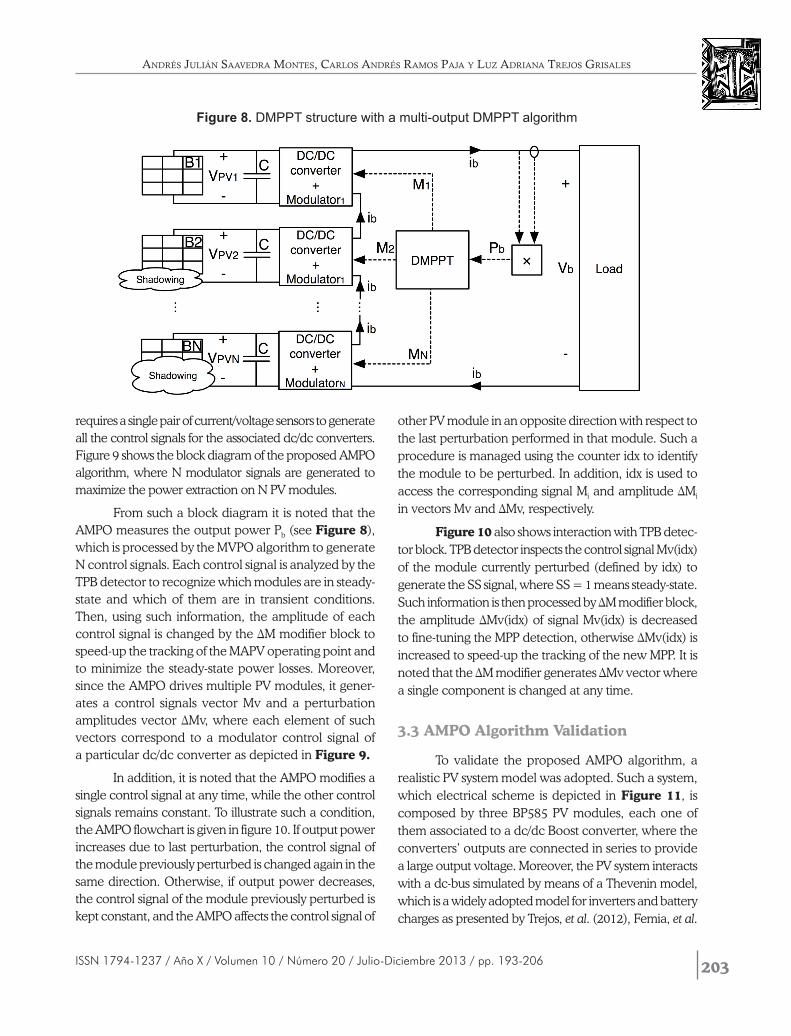
But the DMPPT topology introduced by Femia, et al. (2008) considers a traditional PO controller for each dc/dc converter. Therefore a pair of current/volt-age sensors and a processing unit is required for each PV module, increasing the cost and complexity of the solution. Moreover, the operating points of the dc/dc converters were not taken into account for the output power maximization, which could introduce significant losses. Such aspects were addressed by Petrone, et al. (2012) by means of a multi-output DMPPT algorithm named MVPO, where the basic idea was to maximize the power at the output of the dc/dc converters instead of at the PV terminals. Moreover, a single DMPPT controller was used to generate the control signals for all the dc/dc converters following the structure given in Figure 8, where N PV modules are controlled and the load block represents a grid-connected inverter.

The MVPO solution reduces the number of pair of current/voltage sensors and processing units to 1 pair of sensors and 1 processing unit, and also takes into account the dc/dc converters’ operating point in the optimization process. Such characteristics improve the extraction of PV power in comparison with the solution presented by Femia, et al. (2008). But since the MVPO uses a fixed ∆M value, in the same way that the classical PO, it is impossible to guarantee both fast transient behavior and low steady-state power losses. Therefore, this paper proposes to extend the APO al-gorithm to act on multiple dc/dc converters, obtaining an Adaptive Multi-Variable PO (AMPO) algorithm for DMPPT applications.

3.2 Adaptive Multi-Variable PO (AMPO) Algorithm

To extend the APO to perform DMPPT in multiple PV modules, the new AMPO algorithm perturbs a single variable at any time, thus the algorithm is able to detect the effect on the output power of changes in a particular module. With such a characteristic the AMPO solution


Figure 8. DMPPT structure with a multi-output DMPPT algorithm

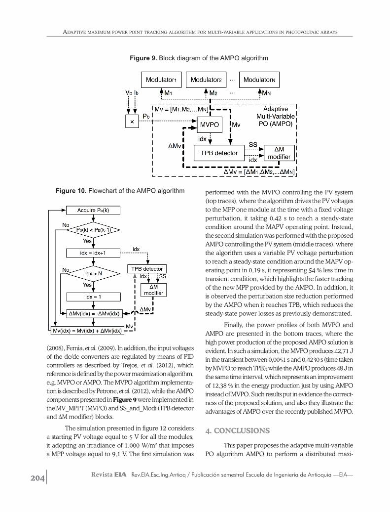
requires a single pair of current/voltage sensors to generate all the control signals for the associated dc/dc converters. Figure 9 shows the block diagram of the proposed AMPO algorithm, where N modulator signals are generated to maximize the power extraction on N PV modules.

From such a block diagram it is noted that the AMPO measures the output power Pb (see Figure 8), which is processed by the MVPO algorithm to generate N control signals. Each control signal is analyzed by the TPB detector to recognize which modules are in steady-state and which of them are in transient conditions. Then, using such information, the amplitude of each control signal is changed by the ∆M modifier block to speed-up the tracking of the MAPV operating point and to minimize the steady-state power losses. Moreover, since the AMPO drives multiple PV modules, it gener-ates a control signals vector Mv and a perturbation amplitudes vector ∆Mv, where each element of such vectors correspond to a modulator control signal of a particular dc/dc converter as depicted in Figure 9.

In addition, it is noted that the AMPO modifies a single control signal at any time, while the other control signals remains constant. To illustrate such a condition, the AMPO flowchart is given in figure 10. If output power increases due to last perturbation, the control signal of the module previously perturbed is changed again in the same direction. Otherwise, if output power decreases, the control signal of the module previously perturbed is kept constant, and the AMPO affects the control signal of

other PV module in an opposite direction with respect to the last perturbation performed in that module. Such a procedure is managed using the counter idx to identify the module to be perturbed. In addition, idx is used to access the corresponding signal Mi and amplitude ∆Mi in vectors Mv and ∆Mv, respectively.

Figure 10 also shows interaction with TPB detec-tor block. TPB detector inspects the control signal Mv(idx) of the module currently perturbed (defined by idx) to generate the SS signal, where SS = 1 means steady-state. Such information is then processed by ∆M modifier block, the amplitude ∆Mv(idx) of signal Mv(idx) is decreased to fine-tuning the MPP detection, otherwise ∆Mv(idx) is increased to speed-up the tracking of the new MPP. It is noted that the ∆M modifier generates ∆Mv vector where a single component is changed at any time.

3.3 AMPO Algorithm Validation

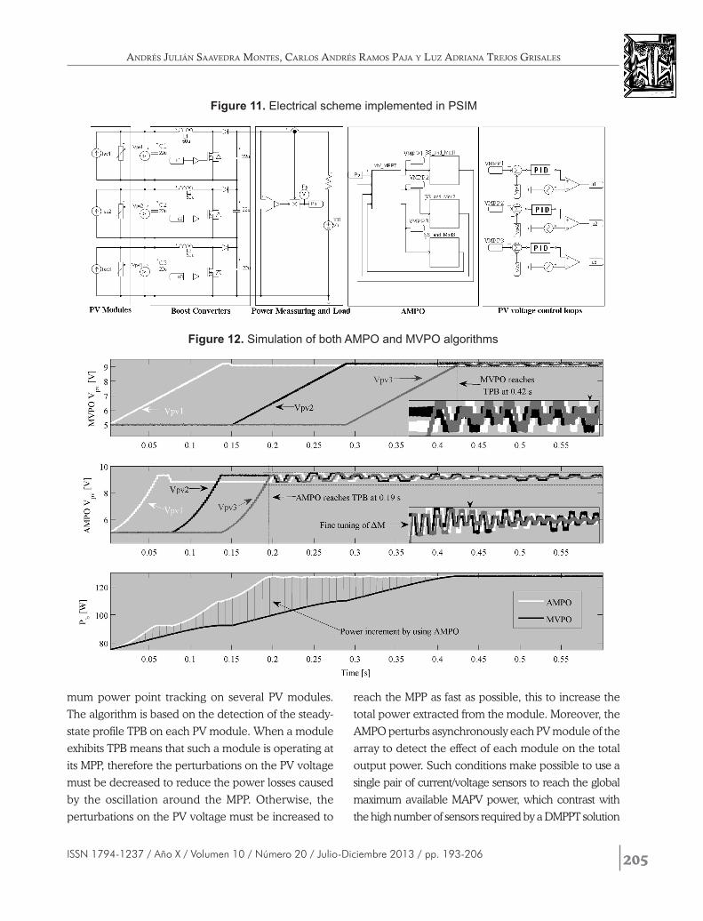
To validate the proposed AMPO algorithm, a realistic PV system model was adopted. Such a system, which electrical scheme is depicted in Figure 11, is composed by three BP585 PV modules, each one of them associated to a dc/dc Boost converter, where the converters’ outputs are connected in series to provide a large output voltage. Moreover, the PV system interacts with a dc-bus simulated by means of a Thevenin model, which is a widely adopted model for inverters and battery charges as presented by Trejos, et al. (2012), Femia, et al.


204



(2008), Femia, et al. (2009). In addition, the input voltages of the dc/dc converters are regulated by means of PID controllers as described by Trejos, et al. (2012), which reference is defined by the power maximization algorithm, e.g. MVPO or AMPO. The MVPO algorithm implementa-tion is described by Petrone, et al. (2012), while the AMPO components presented in Figure 9 were implemented in the MV_MPPT (MVPO) and SS_and_Modi (TPB detector and ∆M modifier) blocks.

The simulation presented in figure 12 considers a starting PV voltage equal to 5 V for all the modules, it adopting an irradiance of 1.000 W/m2 that imposes a MPP voltage equal to 9,1 V. The first simulation was

Figure 9. Block diagram of the AMPO algorithm

Figure 10. Flowchart of the AMPO algorithm performed with the MVPO controlling the PV system (top traces), where the algorithm drives the PV voltages to the MPP one module at the time with a fixed voltage perturbation, it taking 0,42 s to reach a steady-state condition around the MAPV operating point. Instead, the second simulation was performed with the proposed AMPO controlling the PV system (middle traces), where the algorithm uses a variable PV voltage perturbation to reach a steady-state condition around the MAPV op-erating point in 0,19 s, it representing 54 % less time in transient condition, which highlights the faster tracking of the new MPP provided by the AMPO. In addition, it is observed the perturbation size reduction performed by the AMPO when it reaches TPB, which reduces the steady-state power losses as previously demonstrated.

Finally, the power profiles of both MVPO and AMPO are presented in the bottom traces, where the high power production of the proposed AMPO solution is evident. In such a simulation, the MVPO produces 42,71 J in the transient between 0,0051 s and 0,4230 s (time taken by MVPO to reach TPB); while the AMPO produces 48 J in the same time interval, which represents an improvement of 12,38 % in the energy production just by using AMPO instead of MVPO. Such results put in evidence the correct-ness of the proposed solution, and also they illustrate the advantages of AMPO over the recently published MVPO.

4. CONCLUSIONS

This paper proposes the adaptive multi-variable PO algorithm AMPO to perform a distributed maxi-


Figure 11. Electrical scheme implemented in PSIM

Figure 12. Simulation of both AMPO and MVPO algorithms

mum power point tracking on several PV modules.

The algorithm is based on the detection of the steady-

state profile TPB on each PV module. When a module

exhibits TPB means that such a module is operating at

its MPP, therefore the perturbations on the PV voltage

must be decreased to reduce the power losses caused

by the oscillation around the MPP. Otherwise, the

perturbations on the PV voltage must be increased to

reach the MPP as fast as possible, this to increase the

total power extracted from the module. Moreover, the

AMPO perturbs asynchronously each PV module of the

array to detect the effect of each module on the total

output power. Such conditions make possible to use a

single pair of current/voltage sensors to reach the global

maximum available MAPV power, which contrast with

the high number of sensors required by a DMPPT solution


206



composed by multiple PO. In addition, due to the adaptive

nature of the AMPO, it is much faster in the tracking of the

MAPV in comparison with other multi-output algorithms

such as the MVPO solution. Similarly, the AMPO reaches

the minimum amplitudes of the modules perturbations

allowed in steady-state, which reduces the power losses in

comparison with fixed-size perturbations algorithms such

as the MVPO algorithm. Finally, the AMPO solution was

validated by means of simulations using detailed models.

5. ACKNOWLEDGMENTS

This work was supported by GAUNAL group

of the Universidad Nacional de Colombia under the

projects RECONF-PV-18789 and MICRO-RED-18687,

and by COLCIENCIAS under the doctoral scholarships

095-2005 and Convocatoria Nacional 2012-567.

REFERENCES

Petrone, G.; Ramos-Paja, C. A.; Spagnuolo, G. and Vitelli, M. (2012). Granular Control of Photovoltaic Arrays by Means of a Multi-Output Maximum Power Point Tracking Algorithm. Progress in Photovoltaics: Research and Applications, Article in Press, DOI: 10.1002/pip.2179.

Piegari, L. and Rizzo, R. (2010). Adaptive Perturb and Observe Algorithm for Photovoltaic Maximum Power Point Tracking. IET Renewable Power Generation, vol. 4(4), pp 317-328.

Subudhi, B. and Pradhan, R. (2013). A Comparative Study on Maximum Power Point Tracking Techniques for Photovoltaic Power Systems. IEEE Transactions on Sustainable Energy, 4, pp 89-98.

Trejos, A.; González, D. and Ramos-Paja, C. A. (2012) Mod-eling of Step-up Grid-Connected Photovoltaic Systems for Control Purposes. Energies, 5(6), pp 1900-1926.

Abdelsalam, A. K.; Massoud, A. M.; Ahmed, S. and Enjeti, P. N. (2011). High-Performance Adaptive Perturb and Observe MPPT Technique for Photovoltaic-Based Microgrids. IEEE Transactions on Power Electronics, 26(4), pp 1010-1021.

Femia, N.; Granozio, D.; Petrone, G. and Vitelli, M. (2007) Predictive & Adaptive MPPT Perturb and Observe Method. IEEE Transactions on Aerospace and Electronic Systems, 43(3), pp 934-950.

Femia, N.; Lisi, G.; Petrone, G.; Spagnuolo, G. and Vitelli, M. (2008). Distributed Maximum Power Point Tracking of Photovoltaic Arrays: Novel Approach and System Analysis. IEEE Transactions on Industrial Electronics, 55(7), pp 2610-2621.

Femia, N.; Petrone, G.; Spagnuolo, G. and Vitelli, M. (2005) Optimization of perturb and observe maximum power point tracking method. IEEE Transactions on Power Electronics, 20(4), pp 963-973.

Femia, N.; Petrone, G.; Spagnuolo, G. and Vitelli, M. (2009). A Technique for Improving P&O MPPT Performances of Double-Stage Grid-Connected Photovoltaic Systems. IEEE Transactions on Industrial Electronics, 56(11), pp 4473-4482.

Jiang, Y.; Abu Qahouq, J. A. and Haskew, T. A. (2013) Adaptive Step Size With Adaptive-Perturbation-Frequency Digital MPPT Controller for a Single-Sensor Photovoltaic Solar System. IEEE Transactions on Power Electronics, 28(7), pp 3195-3205.

Lee, K.-J. and Kim, R.-Y. (2012). An Adaptive Maximum Power Point Tracking Scheme Based on a Variable Scaling Factor for Photovoltaic Systems. IEEE Transactions on Energy Conversion, 27(4), pp 1002-1008.

Petrone, G. & Ramos-Paja, C. A. (2011). Modeling of Photovoltaic Fields in Mismatched Conditions for Energy Yield Evaluations. Electric Power Systems Research, 81 (4), pp 1003-1013.

PARA CITAR ESTE ARTÍCULO / TO REFERENCE THIS ARTICLE /

PARA CITAR ESTE ARTIGO /

Saavedra-Montes, A.J.; Ramos-Paja, C.A. y Trejos-Grisales, L.A. (2013). Adaptive Maximum Power Point Tracking Algo-rithm for Multi-Variable Applications in Photovoltaic Arrays. Revista EIA, 10(20) julio-diciembre, pp. 209-222. [Online]. Dis-ponible en: http://dx.doi.org/10.14508/reia.2013.10.20.209-222