AdvancedGIS
UsingESRI ArcGIS 9.3Spatial Analyst
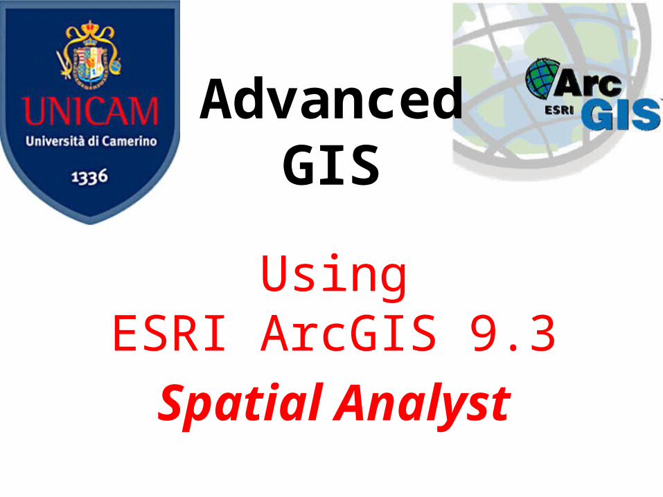
Spatial AnalystActivation
Load and relocate the Spatial Analysttoolbar.
Be sure to have activated the “Spatial Analyst” extension (Menu – Tools – Extensions)
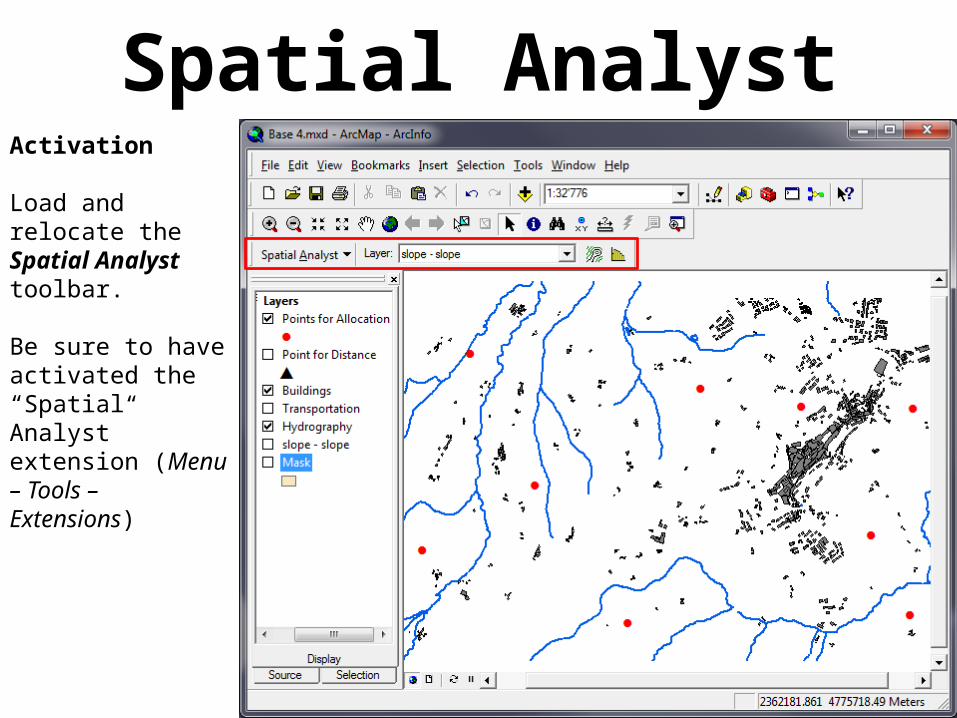
Spatial AnalystOptions
Load the “Base 4” project
In the Options, set the extent to that of “Mask” and the cell size to 5.
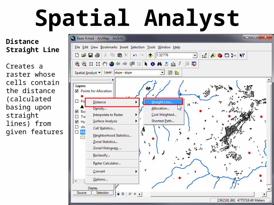
Spatial AnalystDistanceStraight Line
Creates a raster whose cells contain the distance (calculated basing upon straight lines) from given features

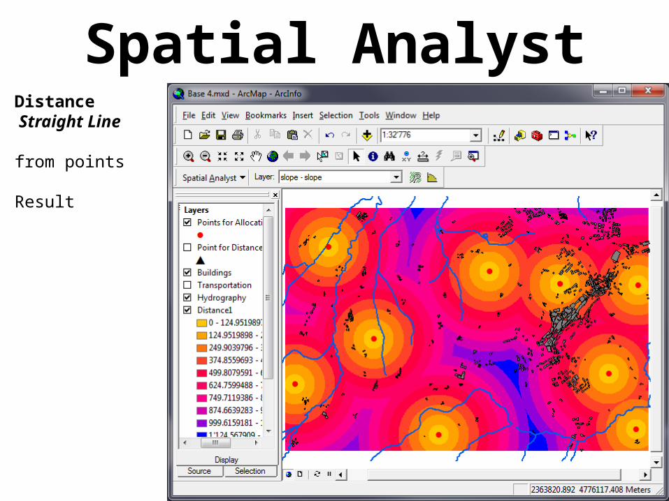
Spatial AnalystDistance Straight Line
from points
Spatial AnalystDistance Straight Line
from points
Result
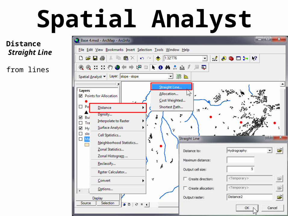
Spatial AnalystDistance Straight Line
from lines
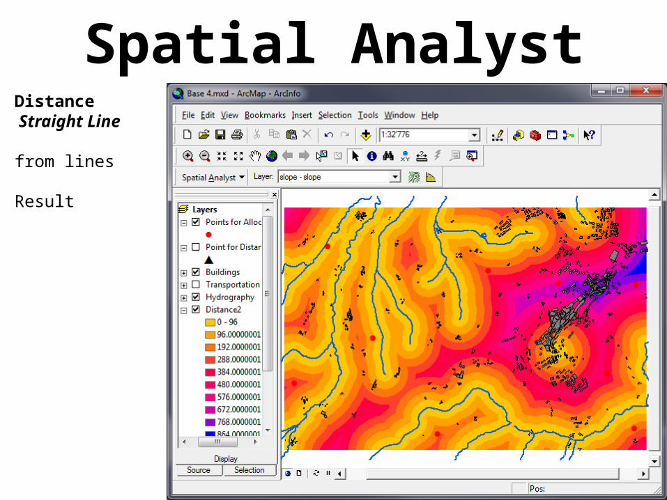
Spatial AnalystDistance Straight Line
from lines
Result
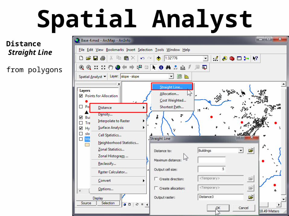
Spatial AnalystDistance Straight Line
from polygons
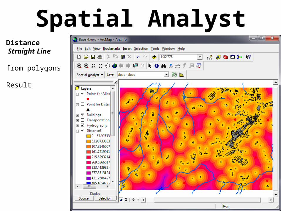
Spatial AnalystDistance Straight Line
from polygons
Result
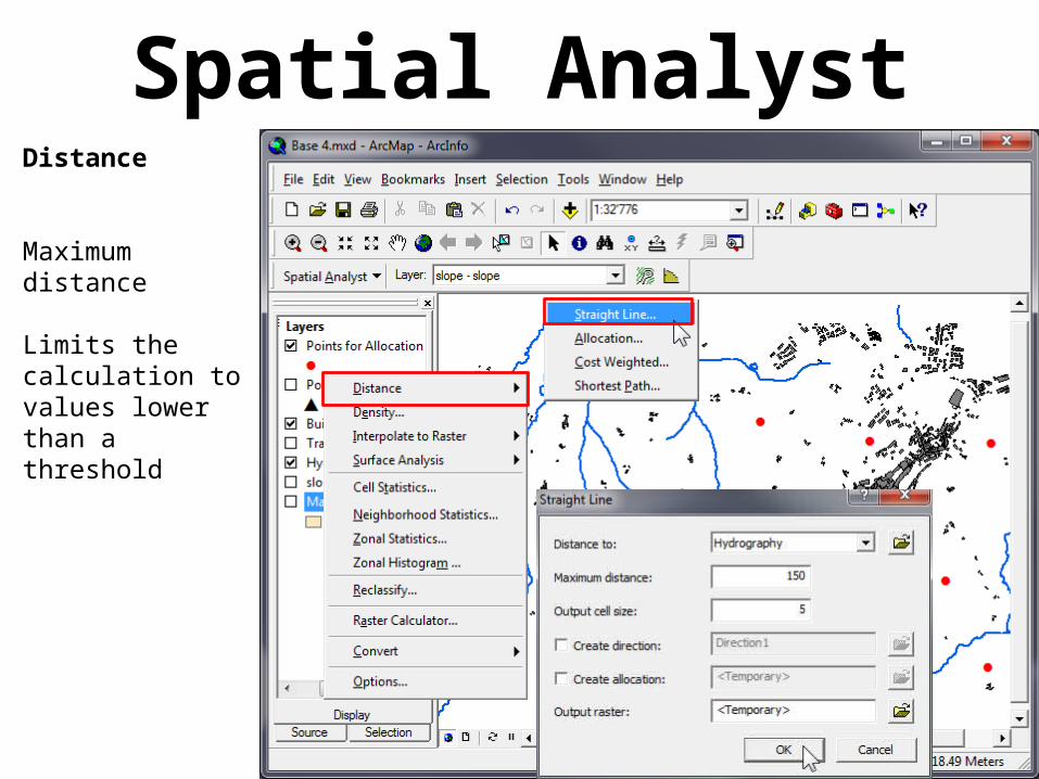
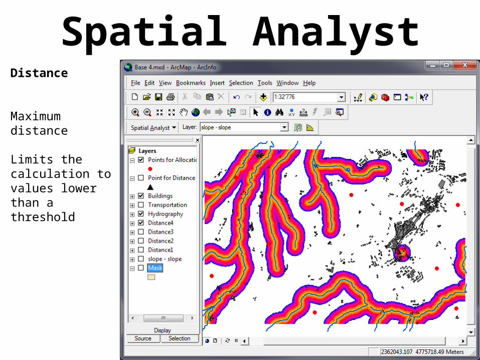
Spatial AnalystDistance
Maximum distance
Limits the calculation to values lower than a threshold
Spatial AnalystDistance
Maximum distance
Limits the calculation to values lower than a threshold
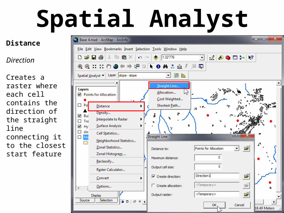
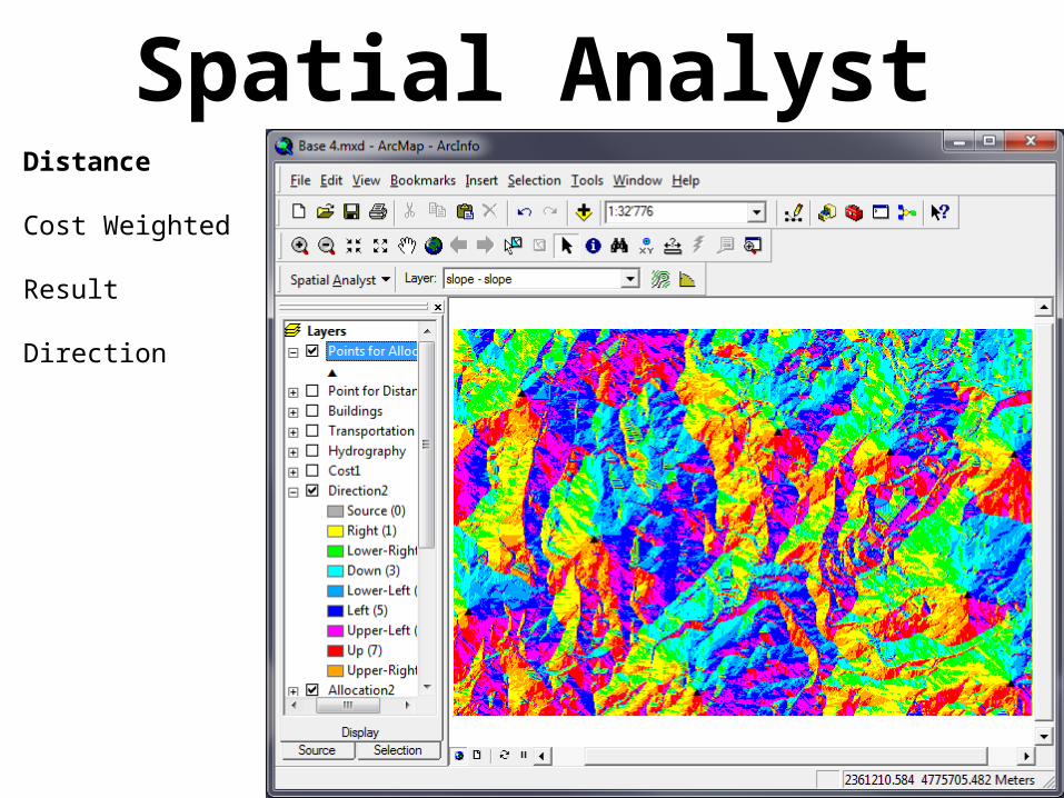
Spatial AnalystDistance
Direction
Creates a raster where each cell contains the direction of the straight line connecting it to the closest start feature
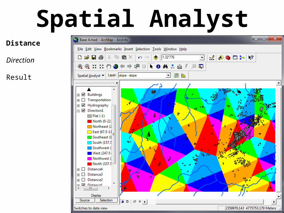
Spatial AnalystDistance
Direction
Result
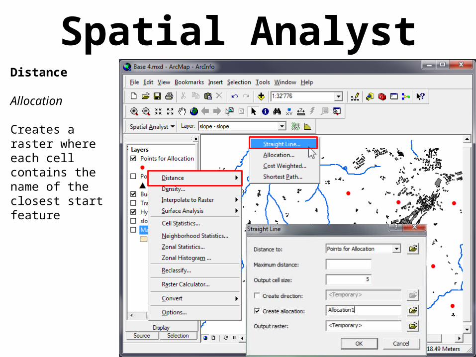
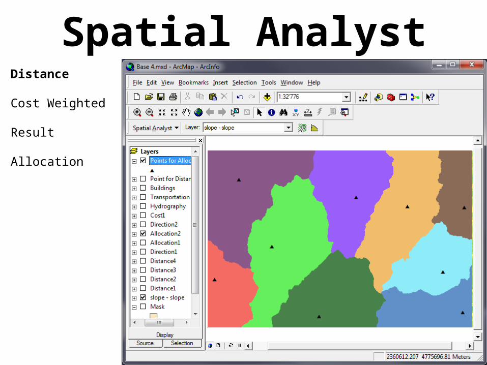
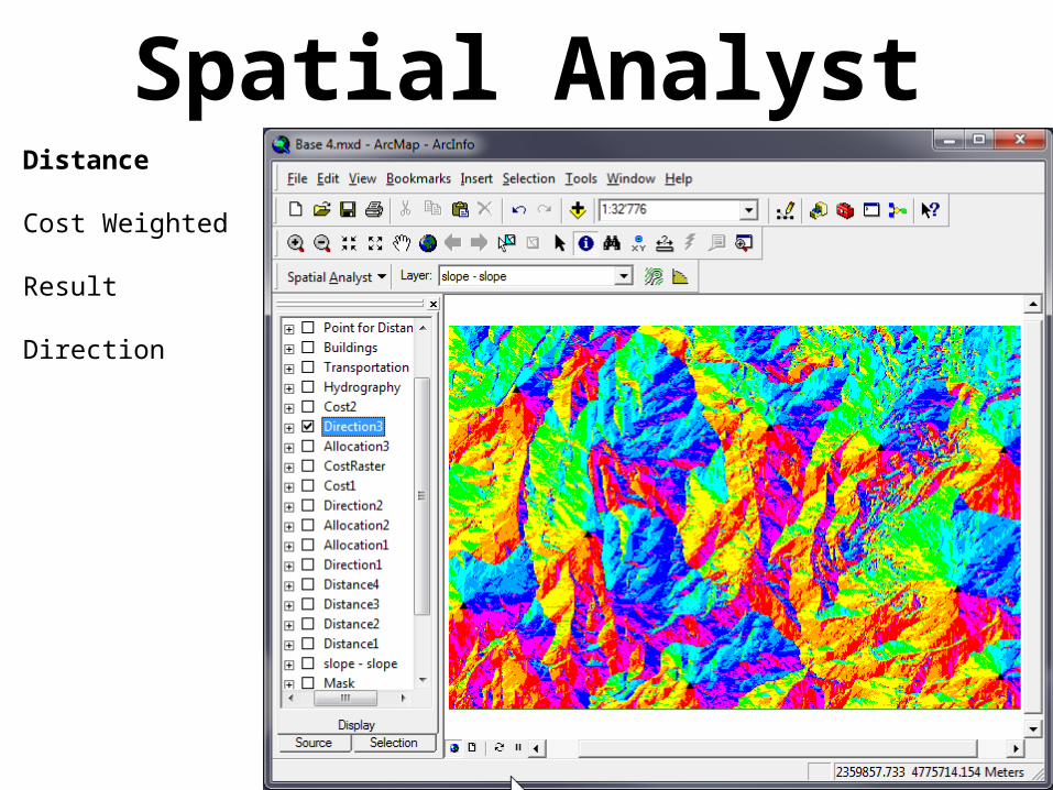
Spatial AnalystDistance
Allocation
Creates a raster where each cell contains the name of the closest start feature
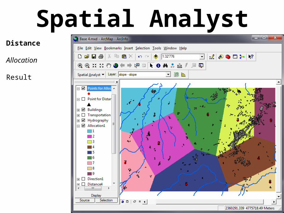
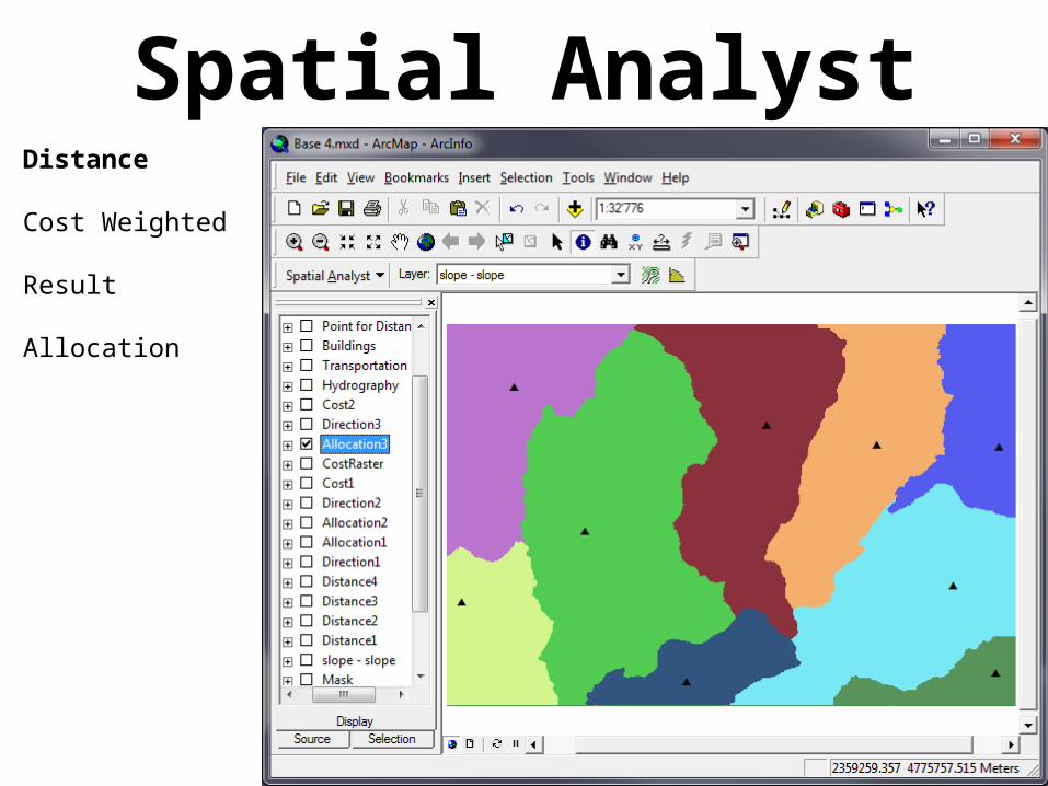
Spatial AnalystDistance
Allocation
Result
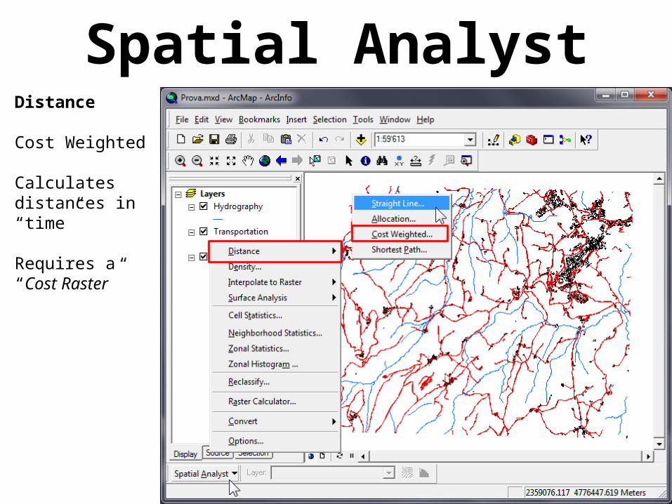
Spatial AnalystDistance
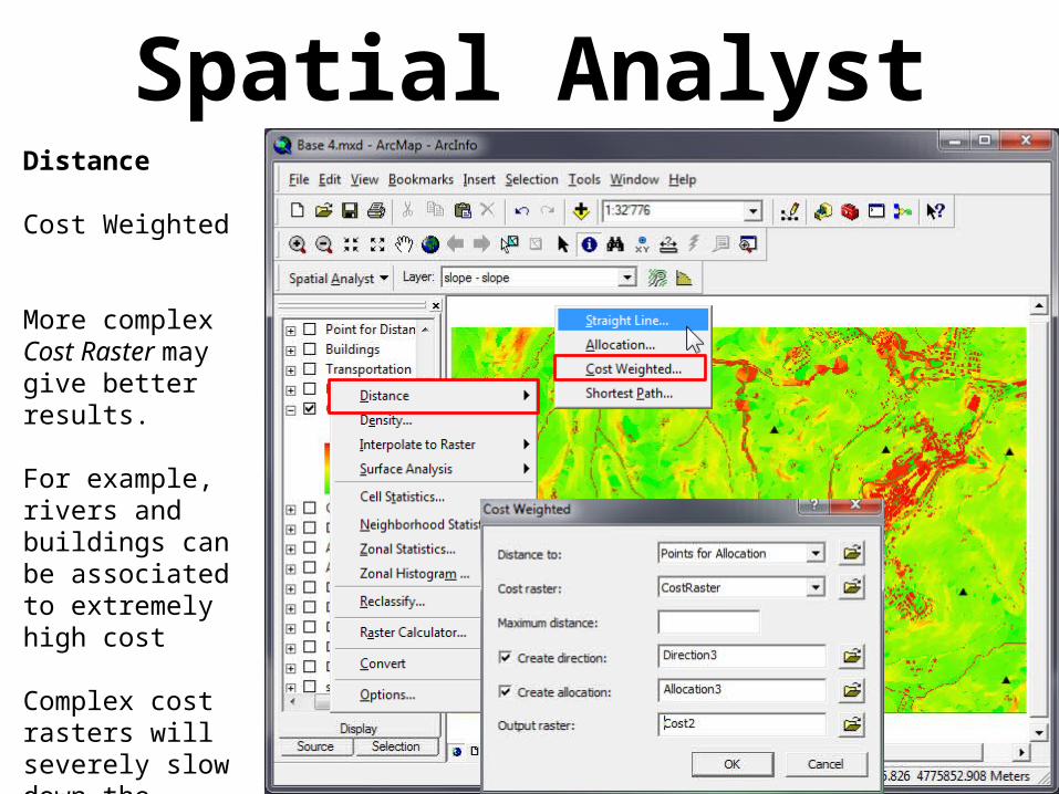
Cost Weighted
Calculates distances in “time”
Requires a “Cost Raster”
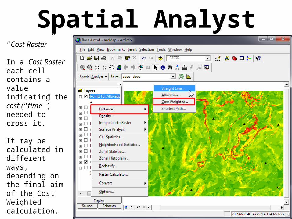
Spatial Analyst“Cost Raster”
In a Cost Raster each cell contains a value indicating the cost (“time”) needed to cross it.
It may be calculated in different ways, depending on the final aim of the Cost Weighted calculation.
The simplest one may be a slope map
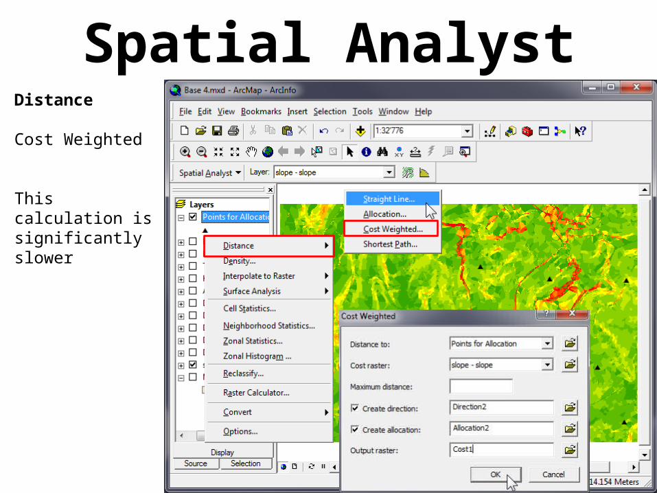
Spatial AnalystDistance
Cost Weighted
This calculation is significantly slower
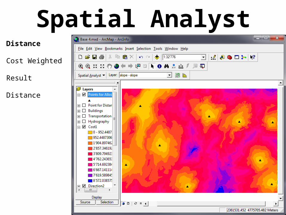
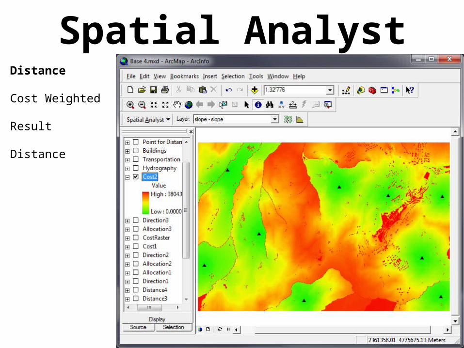
Spatial AnalystDistance
Cost Weighted
Result
Distance
Spatial AnalystDistance
Cost Weighted
Result
Direction
Spatial AnalystDistance
Cost Weighted
Result
Allocation
Spatial AnalystDistance
Cost Weighted
More complex Cost Raster may give better results.
For example, rivers and buildings can be associated to extremely high cost
Complex cost rasters will severely slow down the calculation(s)
Spatial AnalystDistance
Cost Weighted
Result
Distance
Spatial AnalystDistance
Cost Weighted
Result
Direction
Spatial AnalystDistance
Cost Weighted
Result
Allocation
Spatial AnalystDistance
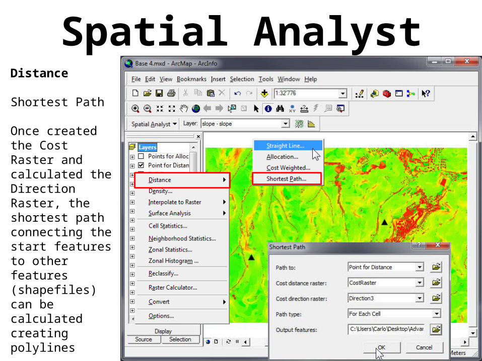
Shortest Path
Once created the Cost Raster and calculated the Direction Raster, the shortest path connecting the start features to other features (shapefiles) can be calculated creating polylines
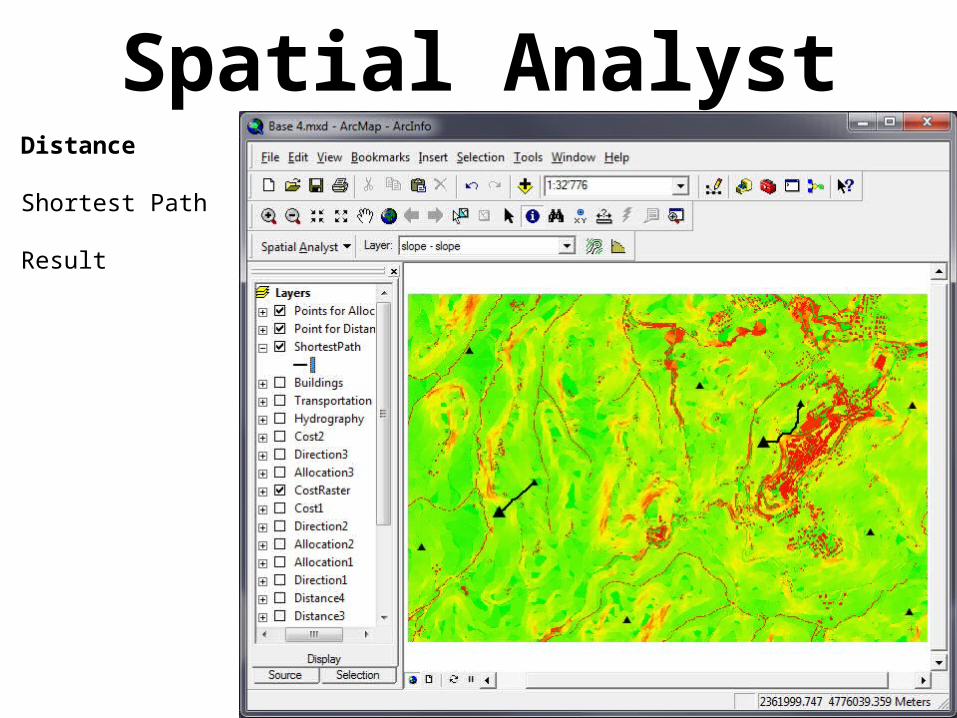
Spatial AnalystDistance
Shortest Path
Result
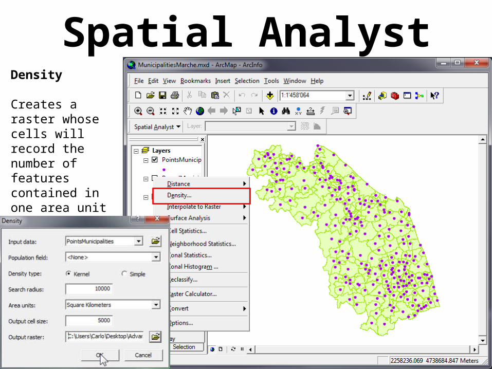
Spatial AnalystDensity
Creates a raster whose cells will record the number of features contained in one area unit
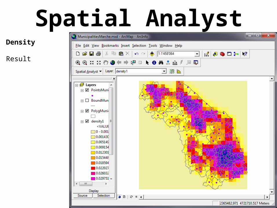
Spatial AnalystDensity
Result
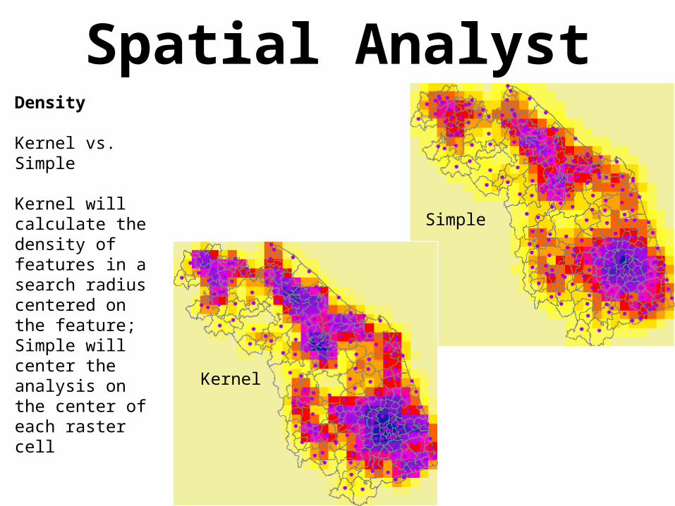
Spatial AnalystDensity
Kernel vs. Simple
Kernel will calculate the density of features in a search radius centered on the feature;Simple will center the analysis on the center of each raster cell
Simple
Kernel
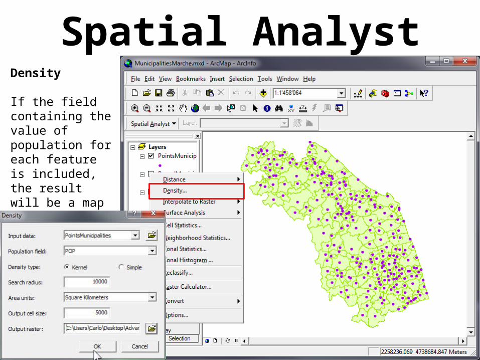
Spatial AnalystDensity
If the field containing the value of population for each feature is included, the result will be a map of population density
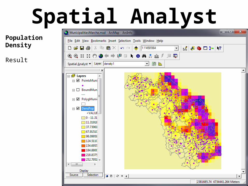
Spatial AnalystPopulation Density
Result
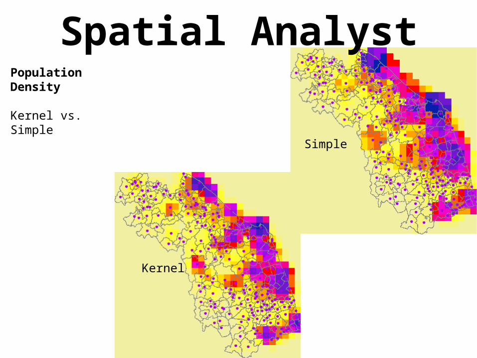
Spatial AnalystPopulation Density
Kernel vs. Simple
Simple
Kernel
Spatial AnalystDensity and Population Density
Density and Population Density can be evaluated for linear features too.
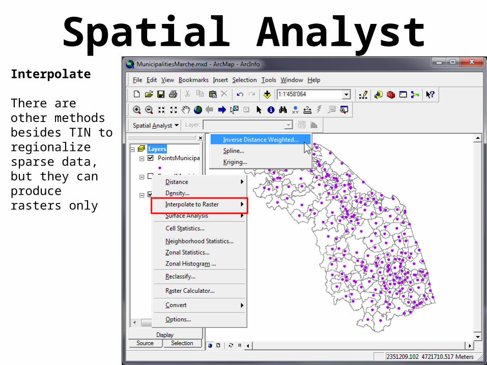
Spatial AnalystInterpolate
There are other methods besides TIN to regionalize sparse data, but they can produce rasters only
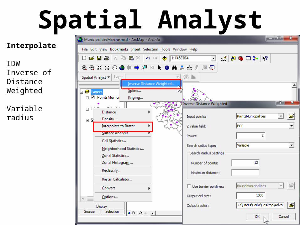
Spatial AnalystInterpolate
IDWInverse of Distance Weighted
Variable radius
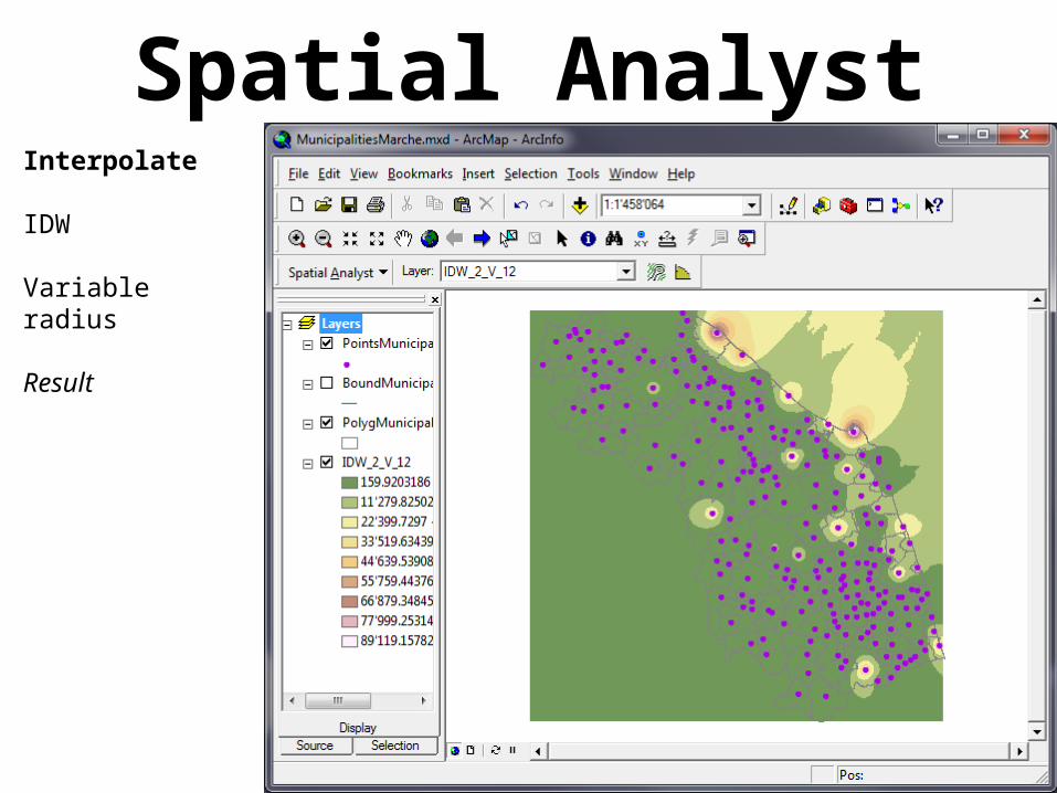
Spatial AnalystInterpolate
IDW
Variable radius
Result
Spatial AnalystInterpolate
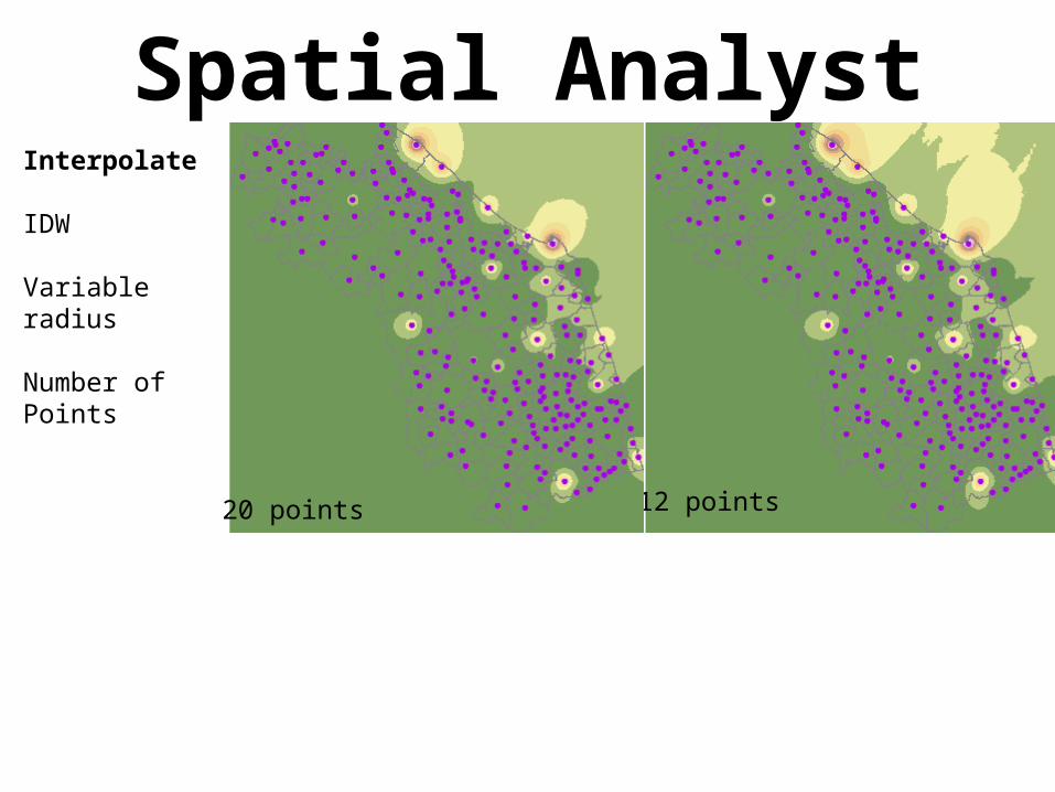
IDW
Variable radius
Number of Points
12 points20 points
Spatial AnalystInterpolate
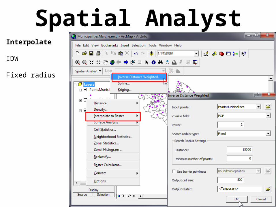
IDW
Fixed radius
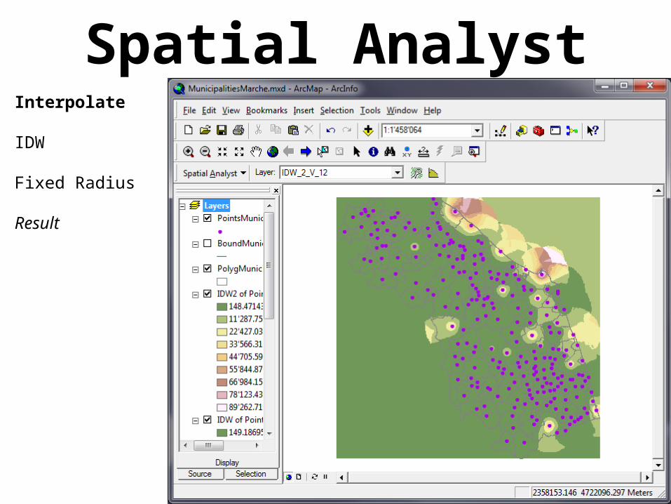
Spatial AnalystInterpolate
IDW
Fixed Radius
Result
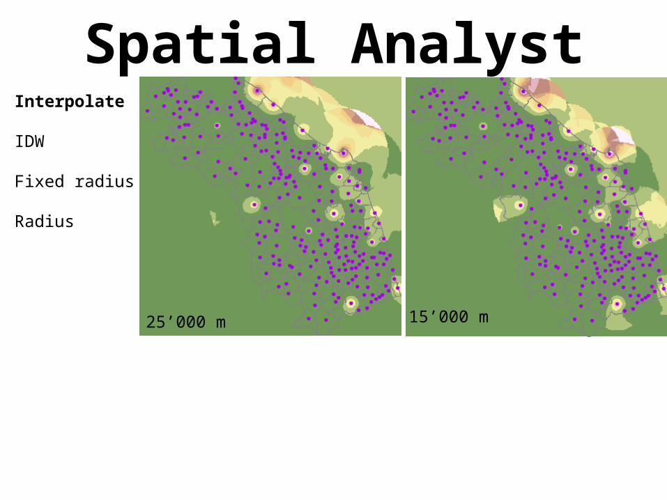
Spatial AnalystInterpolate
IDW
Fixed radius
Radius
15’000 m25’000 m
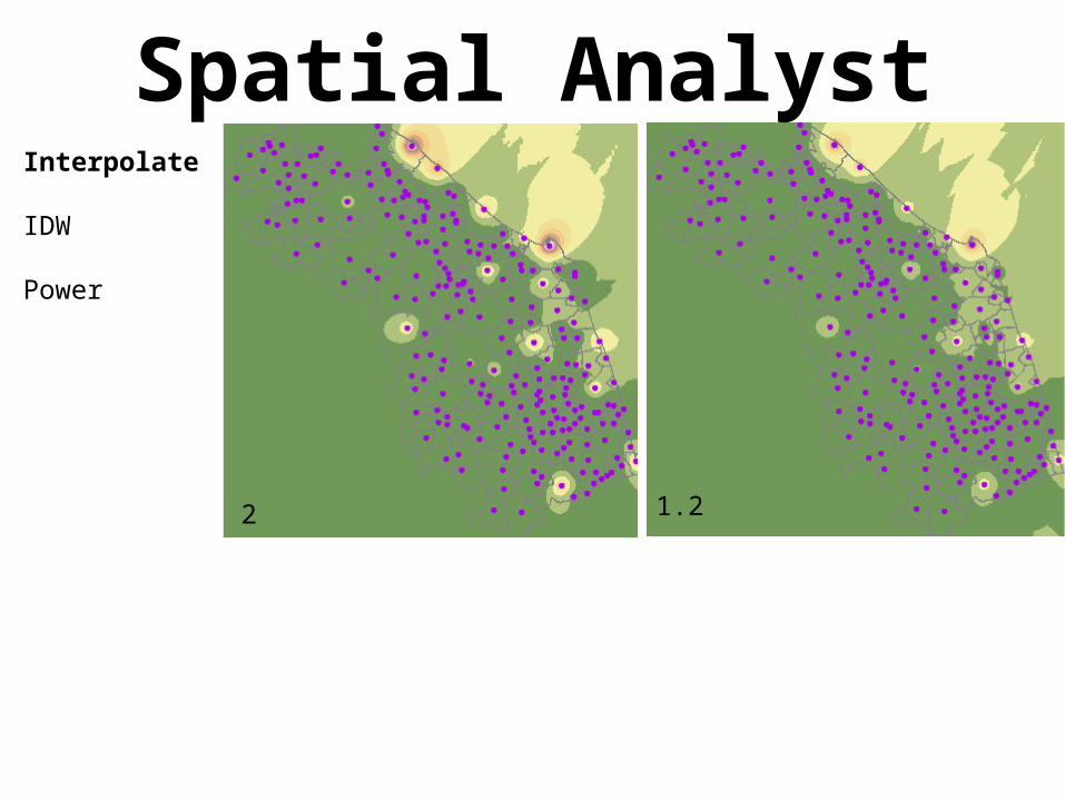
Spatial AnalystInterpolate
IDW
Power
1.22
Spatial AnalystInterpolate
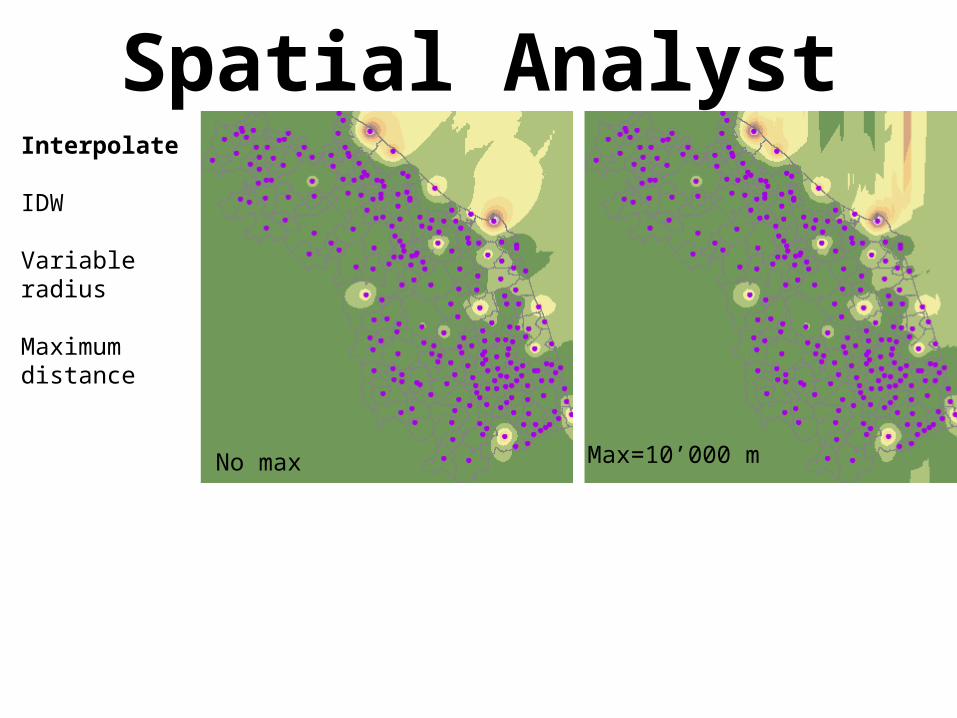
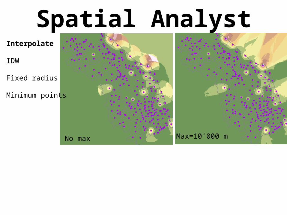
IDW
Variable radius
Maximum distance
Max=10’000 mNo max
Spatial AnalystInterpolate
IDW
Fixed radius
Minimum points
Max=10’000 mNo max
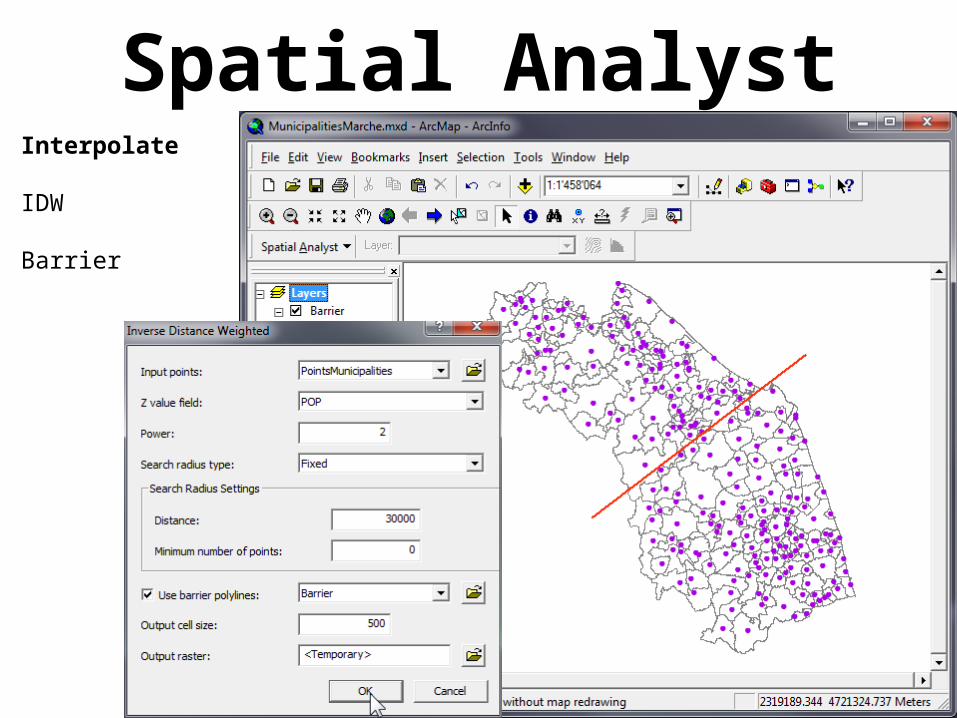
Spatial AnalystInterpolate
IDW
Barrier
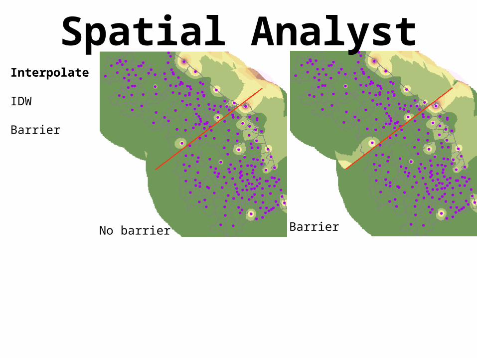
Spatial AnalystInterpolate
IDW
Barrier
BarrierNo barrier
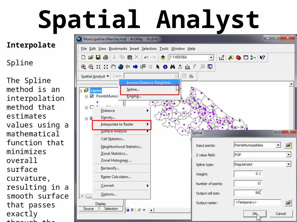
Spatial AnalystInterpolate
Spline
The Spline method is an interpolation method that estimates values using a mathematical function that minimizes overall surface curvature, resulting in a smooth surface that passes exactly through the input points.
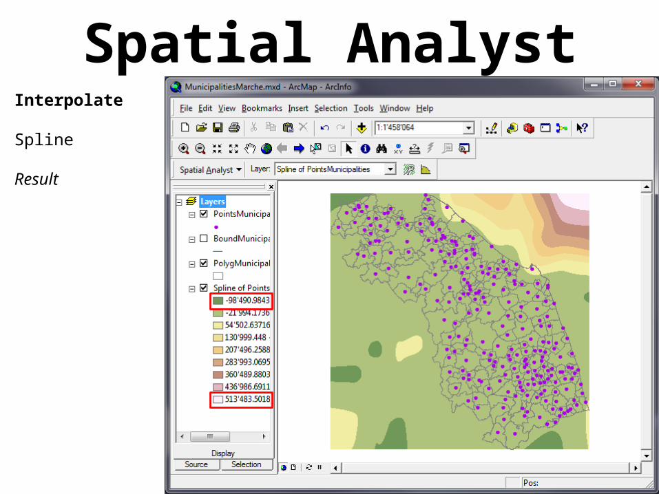
Spatial AnalystInterpolate
Spline
Result

Spatial AnalystInterpolate
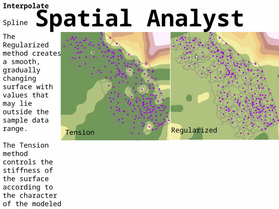
Spline
The Regularized method creates a smooth, gradually changing surface with values that may lie outside the sample data range.
The Tension method controls the stiffness of the surface according to the character of the modeled phenomenon. It creates a less smooth surface with values more closely constrained by the sample data range.
Tension Regularized
Spatial AnalystInterpolate
Spline
The Regularized method creates a smooth, gradually changing surface with values that may lie outside the sample data range.
The Tension method controls the stiffness of the surface according to the character of the modeled phenomenon. It creates a less smooth surface with values more closely constrained by the sample data range.
Tension Regularized
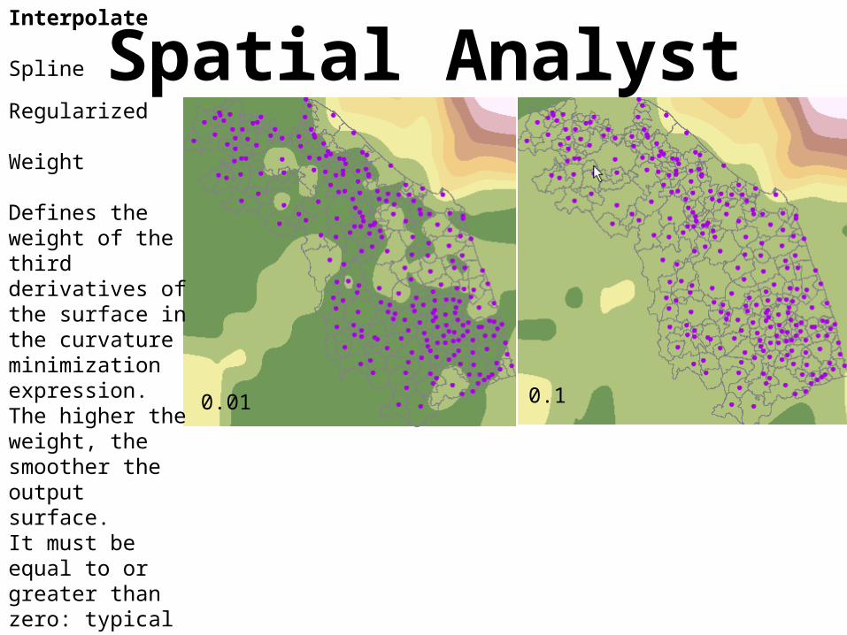
Spatial AnalystInterpolate
Spline
Regularized
Weight
Defines the weight of the third derivatives of the surface in the curvature minimization expression. The higher the weight, the smoother the output surface. It must be equal to or greater than zero: typical values are 0, 0.001, 0.01, 0.1, and 0.5.
0.01 0.1
Spatial AnalystInterpolate
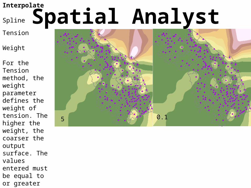
Spline
Tension
Weight
For the Tension method, the weight parameter defines the weight of tension. The higher the weight, the coarser the output surface. The values entered must be equal to or greater than zero. The typical values are 0, 1, 5, and 10.
5 0.1
Spatial AnalystInterpolate
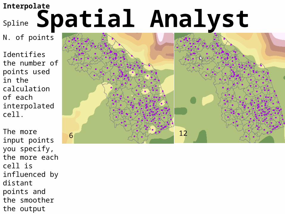
Spline
N. of points
Identifies the number of points used in the calculation of each interpolated cell.
The more input points you specify, the more each cell is influenced by distant points and the smoother the output surface. The larger the number of points, the longer it will take to process the output raster.
6 12
Spatial AnalystInterpolate
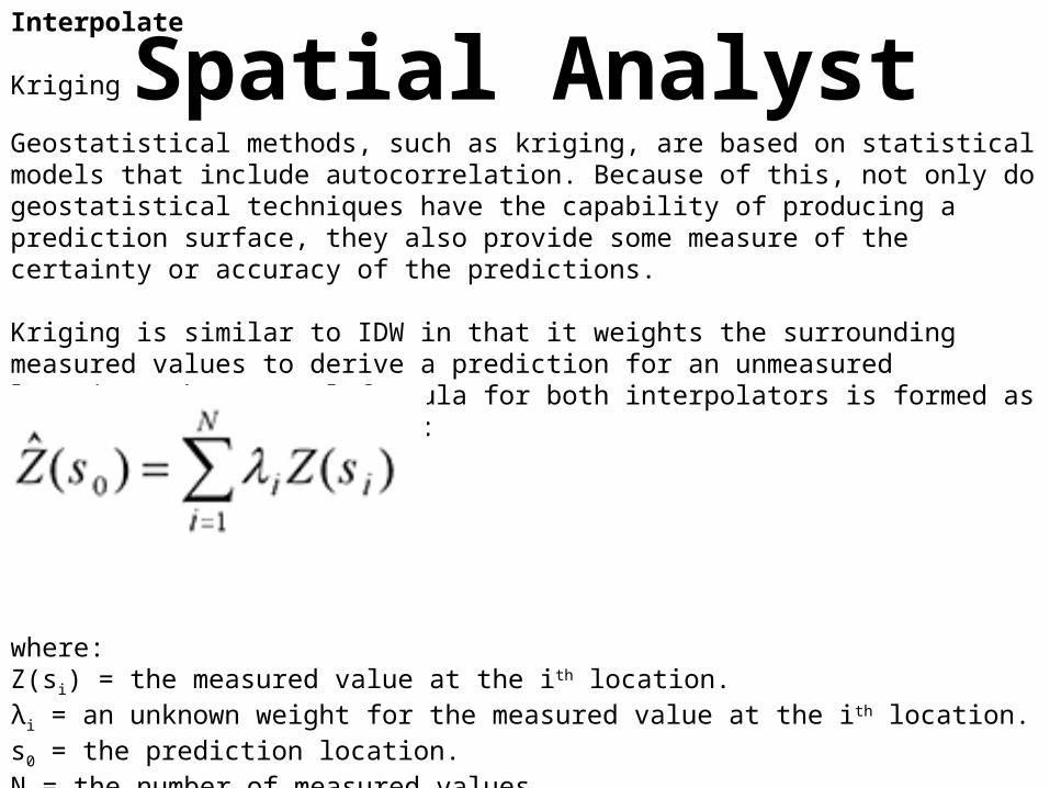
Kriging
Geostatistical methods, such as kriging, are based on statistical models that include autocorrelation. Because of this, not only do geostatistical techniques have the capability of producing a prediction surface, they also provide some measure of the certainty or accuracy of the predictions.
Kriging is similar to IDW in that it weights the surrounding measured values to derive a prediction for an unmeasured location. The general formula for both interpolators is formed as a weighted sum of the data:
where: Z(si) = the measured value at the ith location. λi = an unknown weight for the measured value at the ith location. s0 = the prediction location. N = the number of measured values.
Spatial AnalystInterpolate
Kriging
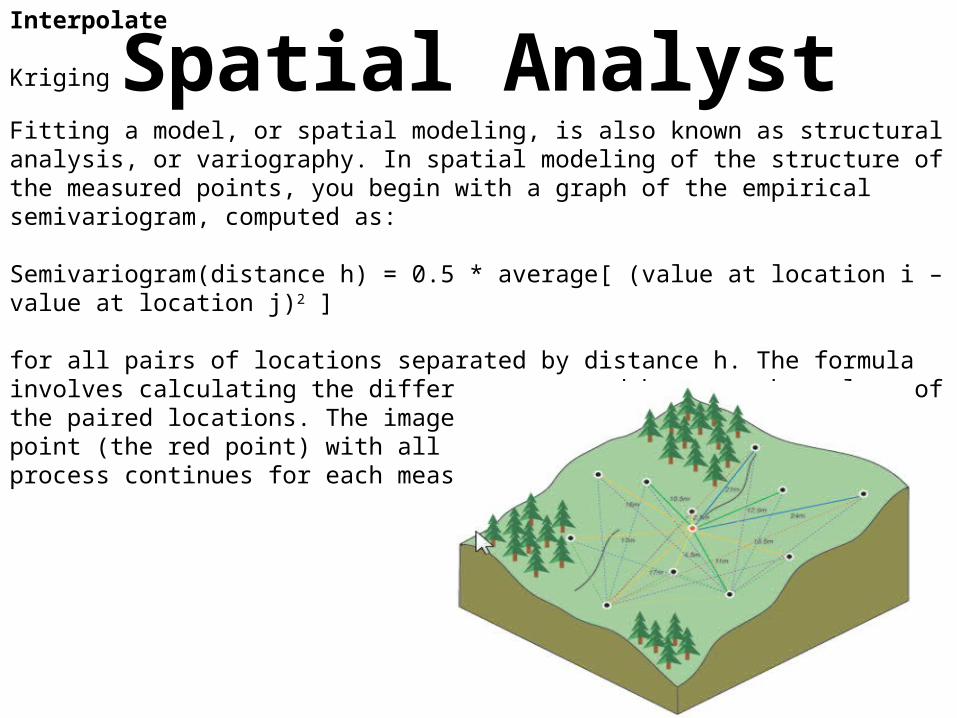
Fitting a model, or spatial modeling, is also known as structural analysis, or variography. In spatial modeling of the structure of the measured points, you begin with a graph of the empirical semivariogram, computed as: Semivariogram(distance h) = 0.5 * average[ (value at location i – value at location j)2 ]
for all pairs of locations separated by distance h. The formula involves calculating the difference squared between the values of the paired locations. The image below shows the pairing of one point (the red point) with all other measured locations. This process continues for each measured point.
Spatial AnalystInterpolate
Kriging
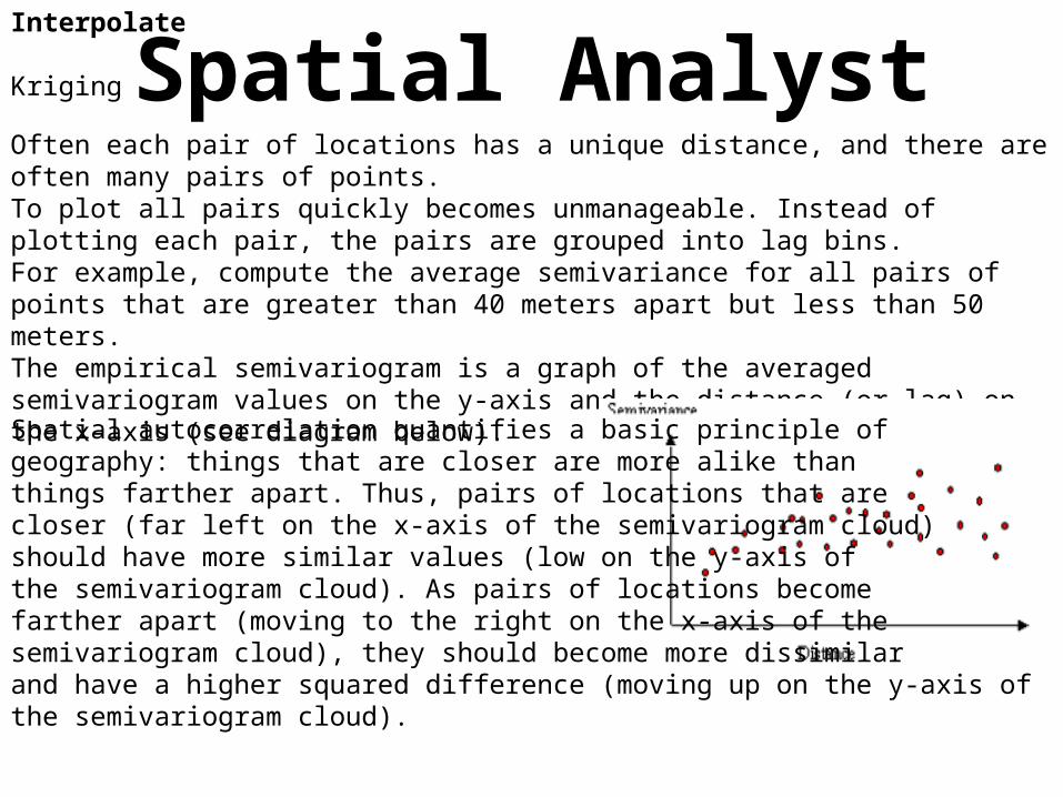
Often each pair of locations has a unique distance, and there are often many pairs of points. To plot all pairs quickly becomes unmanageable. Instead of plotting each pair, the pairs are grouped into lag bins. For example, compute the average semivariance for all pairs of points that are greater than 40 meters apart but less than 50 meters. The empirical semivariogram is a graph of the averaged semivariogram values on the y-axis and the distance (or lag) on the x-axis (see diagram below).
Spatial autocorrelation quantifies a basic principle of geography: things that are closer are more alike than things farther apart. Thus, pairs of locations that are closer (far left on the x-axis of the semivariogram cloud) should have more similar values (low on the y-axis of the semivariogram cloud). As pairs of locations become farther apart (moving to the right on the x-axis of the semivariogram cloud), they should become more dissimilar and have a higher squared difference (moving up on the y-axis of the semivariogram cloud).
Spatial AnalystInterpolate
Kriging
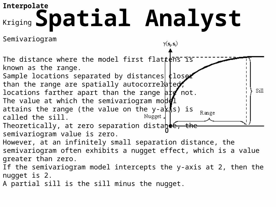
Semivariogram
The distance where the model first flattens is known as the range. Sample locations separated by distances closer than the range are spatially autocorrelated; locations farther apart than the range are not.The value at which the semivariogram model attains the range (the value on the y-axis) is called the sill. Theoretically, at zero separation distance, the semivariogram value is zero. However, at an infinitely small separation distance, the semivariogram often exhibits a nugget effect, which is a value greater than zero. If the semivariogram model intercepts the y-axis at 2, then the nugget is 2. A partial sill is the sill minus the nugget.

Spatial AnalystInterpolate
Kriging
Spatial AnalystInterpolate
Kriging
Methods
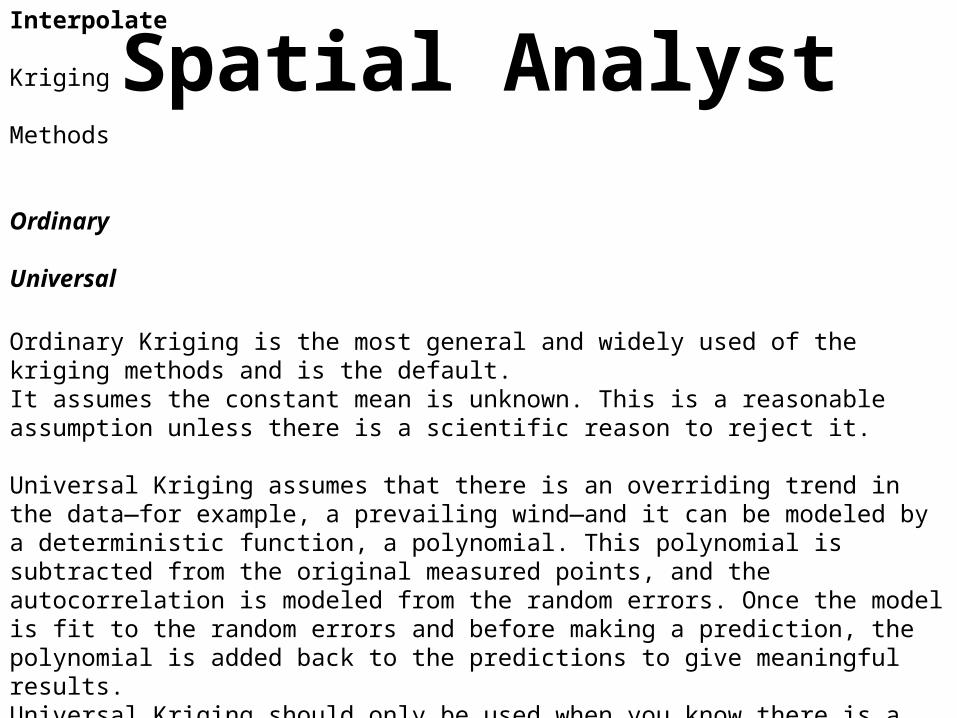
Ordinary
Universal
Ordinary Kriging is the most general and widely used of the kriging methods and is the default. It assumes the constant mean is unknown. This is a reasonable assumption unless there is a scientific reason to reject it.
Universal Kriging assumes that there is an overriding trend in the data—for example, a prevailing wind—and it can be modeled by a deterministic function, a polynomial. This polynomial is subtracted from the original measured points, and the autocorrelation is modeled from the random errors. Once the model is fit to the random errors and before making a prediction, the polynomial is added back to the predictions to give meaningful results. Universal Kriging should only be used when you know there is a trend in your data, and you can give a scientific justification to describe it.
Spatial AnalystInterpolate
Kriging
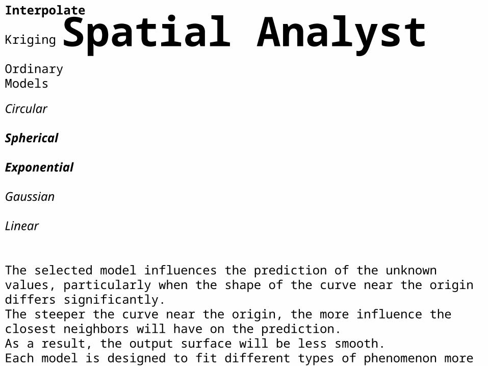
Ordinary Models
Circular
Spherical
Exponential Gaussian Linear
The selected model influences the prediction of the unknown values, particularly when the shape of the curve near the origin differs significantly. The steeper the curve near the origin, the more influence the closest neighbors will have on the prediction. As a result, the output surface will be less smooth.Each model is designed to fit different types of phenomenon more accurately.
Spatial AnalystInterpolate
Kriging
Models
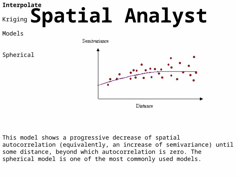
Spherical
This model shows a progressive decrease of spatial autocorrelation (equivalently, an increase of semivariance) until some distance, beyond which autocorrelation is zero. The spherical model is one of the most commonly used models.
Spatial AnalystInterpolate
Kriging
Models
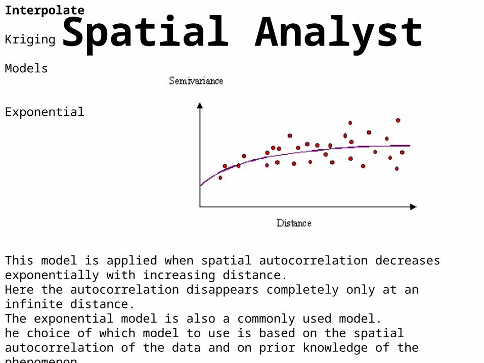
Exponential
This model is applied when spatial autocorrelation decreases exponentially with increasing distance. Here the autocorrelation disappears completely only at an infinite distance. The exponential model is also a commonly used model. he choice of which model to use is based on the spatial autocorrelation of the data and on prior knowledge of the phenomenon.
Spatial AnalystInterpolate
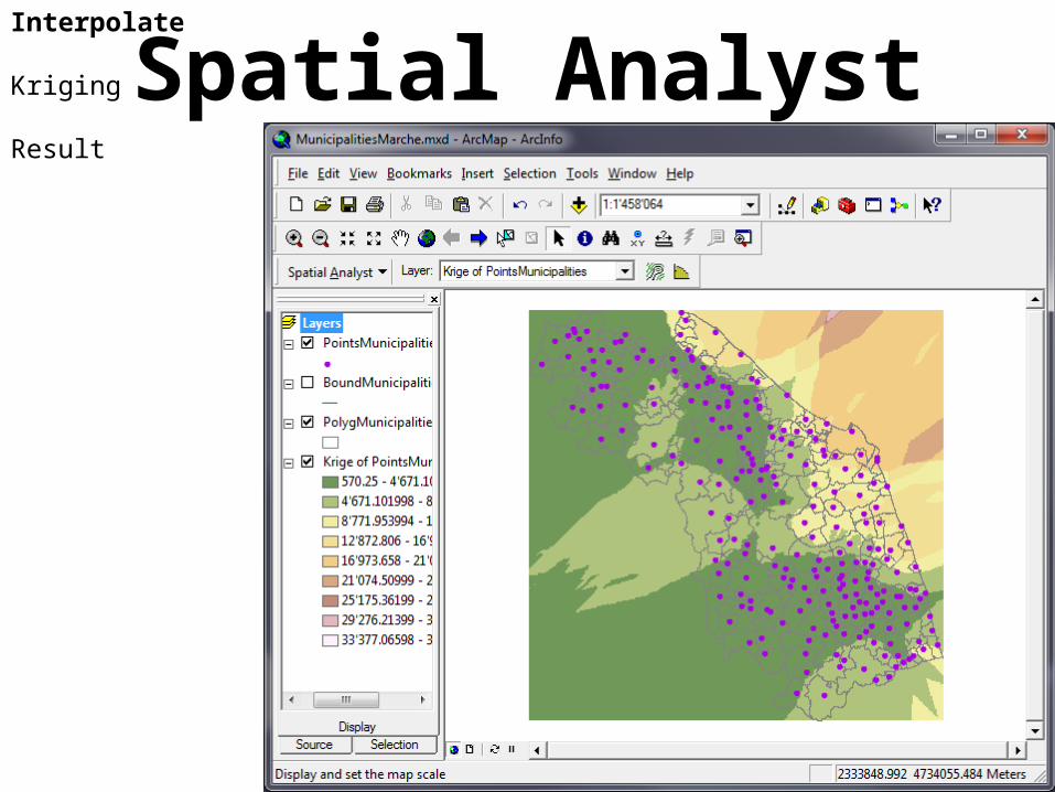
Kriging
Result
Spatial AnalystInterpolate
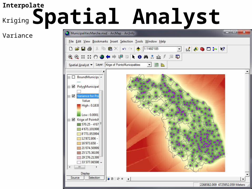
Kriging
Variance
Recommended