Approximate Geometric Pattern Matching under Rigid Motions∗
Michael T. Goodrich† Joseph S. B. Mitchell‡ Mark W. Orletsky§
Abstract
We present techniques for matching point-sets in two and three dimensions under rigid-bodytransformations. We prove bounds on the worst-case performance of these algorithms to bewithin a small constant factor of optimal, and conduct experiments to show that the averageperformance of these matching algorithms is often better than that predicted by the worst-casebounds.
Index Terms: Hausdorff distance, pattern matching, registration.
1 Introduction
Suppose we are given a set B of n points in IRd, which we shall call the background, and a set P
of m points in IRd, which we shall call the pattern. The geometric pattern matching problem is to
determine a rigid motion, taken from some class of motions, such that each point in P is moved to
a point in B.
It is easy to solve this problem if we insist on exactly matching points in P to points in B: Store
B in a dictionary, designate one point of P as a “reference point,” and consider the n placements
of P corresponding to the reference point coinciding with each point of B; for each placement, do
m − 1 queries into the dictionary to determine if all m points of P are matched. Unfortunately,
this approach is very sensitive to noise. Thus, it is more natural to pose the approximate geometric
pattern matching problem: Find a rigid motion of P such that each point of P is moved near
to a point in B. Formally, we desire a rigid motion T , taken from some class of motions C,
such that the directed Hausdorff distance from T (P ) to B is minimized. Recall that the directed
Hausdorff distance1, h(C, D), from a point set C to another point set D is defined as h(C, D) =
maxc∈C mind∈D ρ(c, d), where ρ is the usual Euclidean distance between c and d. Thus, h(C, D) is
the smallest amount by which we need to “grow” the points of D in order that all of C is covered
∗This work was announced in preliminary form in the Proc. Tenth Annual ACM Symposium on Computational
Geometry, 1994, pp. 103-112.†[email protected]. Dept. of Computer Science, Johns Hopkins University, Baltimore, MD 21218. Partially
supported by the U.S. Army Research Office under grant DAAH04–96–1–0013, and by NSF under Grants CCR-9625289 and CCR-9732300.
‡[email protected]. Department of Applied Mathematics and Statistics, State University of New York, StonyBrook, NY 11794-3600. Partially supported by NSF grants CCR-9504192 and CCR-9732220.
§[email protected]. Dept. of Computer Science, Johns Hopkins University, Baltimore, MD 21218. This researchwas partially supported by NSF grant IRI-9116843.
1The undirected Hausdorff distance is defined as H(C, D) = max{h(C, D), h(D, C)}.
1
by the grown set. Using the directed Hausdorff distance as the matching criterion thus allows us
to find the pattern in the background. (In contrast, a least squares fit would not produce this type
of match since all background points, including those that do not correspond to any of the pattern
points, would influence what is considered to be the optimal placement of the pattern.)
1.1 Previous Work
Point set pattern matching has been an important problem in machine vision for some time. A
number of different general strategies have been used to approach the problem. Four such strategies,
along with their advantages and disadvantages are outlined below.
The Cluster Approach. The clustering approach ([28, 29, 31, 34, 36, 38]) involves associating
confidence values with locations in a discretized configuration space of possible orientations of
the pattern with respect to the background and then choosing the match that is associated with
the largest cluster or peak in the confidence values in the configuration space. These strategies
are particularly effective at matching patterns that are partially occluded, or have points missing
for other reasons, and patterns in which some points are severely corrupted, as demonstrated by
the experimental work of the authors. The methods, however, require that the tolerance t be
prespecified, and sometimes “tweaked”, and produce matches in which those points that do not fall
within t of an associated point are neglected in terms of the degree to which they actually deviate
from the nearest matching point.
The Absolute Orientation Approach. The absolute orientation approach ([7, 20, 23, 24, 37])
is concerned with determining the pose (see, e.g., [16, 20]) of the pattern with respect to the
background that minimizes the least squares error. These results assume that the size of the pattern
set and the size of the background set are the same, and even more limiting, that a correspondence
between the points in the pattern and the points in the background has already been established.
The Extracted Information Approach. Another general strategy, which we call the extracted
information approach, attempts to match the pattern to the background based on information
extracted from the sets of points. See, e.g., [2, 4, 17, 19, 32]. As shown by the authors, these
methods work very well, theoretically and experimentally, for patterns and backgrounds that are
related to each other by certain, sometimes strict, criteria. These methods do not, in general, work
very well for the cases of missing points, and in some cases, the extracted information will change
severely and abruptly with infinitesimal changes in a single pattern point.
The Computational Geometry Approach. Using computational geometry techniques, Alt et
al. [5] give methods for finding congruences between two sets of points A and B under rigid motions.
In addition to exact methods, they introduce an approximate version of the problem, for a given
tolerance ǫ > 0, and ask to find a motion T , if it exists, that allows a matching between each point
in T (A) and a point in B at distance ≤ ǫ. They also consider the optimization version, to compute
2
the smallest ǫ admitting such a motion; unfortunately, their running times for this version are quite
high. This version of the problem is very close to the problem we address in this paper.
Imai et al. [27] show that these bounds can be reduced somewhat if an assignment of points in
A to points in B is given. Similarly, Arkin et al. [6] show that one can improve the running times
in the approximate case if the “noise regions” are disjoint. Even so, the methods in these papers
are relatively sophisticated, with rather high running times for all but the most simple motions.
In work more directly related to this paper, several researchers [9, 10, 25, 26] have studied
methods for finding rigid motions that minimize either the directed or undirected Hausdorff distance
between the two point sets. All of these methods are based on intersecting higher-degree curves
and/or surfaces, which are then searched (sometimes parametrically [1, 11, 12, 13, 30]) to find
a global minimum. This reliance upon intersection computations leads to algorithms that are
potentially numerically unstable, are conceptually complex, and have running times that are high
for all but the most trivial motions. Indeed, Rucklidge [35] gives evidence that such methods must
have high running times.
The high running times of these methods motivated Heffernan [21] and Heffernan and Schirra [22]
to consider an approximate decision problem for approximate point set congruence (they did not
study point set pattern matching). Their general framework, for a given parameter ǫ > 0, is to
solve the approximate set congruence problem [5], except that one is allowed to “give up” if one
discovers that ǫ is “too close” to the optimal value ǫ∗ (i.e., the Hausdorff distance between T (A)
and B). By allowing algorithms to be “lazy” in this way, they show that the running times can
be significantly improved. Unfortunately, this approach can result in a large computing time that
yields no approximation, with the time increasing substantially if one tries to get a yes-or-no answer
for an ǫ close to ǫ∗. Thus, it is difficult to use their methods to approximate ǫ∗.
1.2 Our Results
In this paper we present a very simple approach for approximate point set pattern matching under
rigid motions, where one is given a pattern set P of m points in IRd and a background B of n points
in IRd and asked to find a rigid motion T that minimizes h(T (P ), B). Our methods are based on
a simple “pinning” strategy. They are fast, easy to implement, and numerically stable. Moreover,
since they are defined for the (more general) directed Hausdorff measure, they are tolerant of noise
in the background.
Our methods are not exact, however. Instead, in the spirit of approximation methods for other
hard optimization problems (e.g., NP-hard problems [14]), we derive algorithms that are guaranteed
to come close to the optimal value, ǫ∗. In particular, each of our methods gives a rigid motion T
such that h(T (P ), B) ≤ αǫ∗, for some small constant α > 1. (We note that a similar use of
approximation algorithms is taken by Alt et al. [3] for the problem of polygon matching.) Our
results are summarized in Table 1.
We justify the implementability of our methods through an empirical study of the running time
and the quality of the match of our methods when run on various input instances. We compare
the performance with that of a more conventional procedure based on a branch-and-bound search
of a discretized configuration space. Our results show that, in practice, our methods are fast and
3
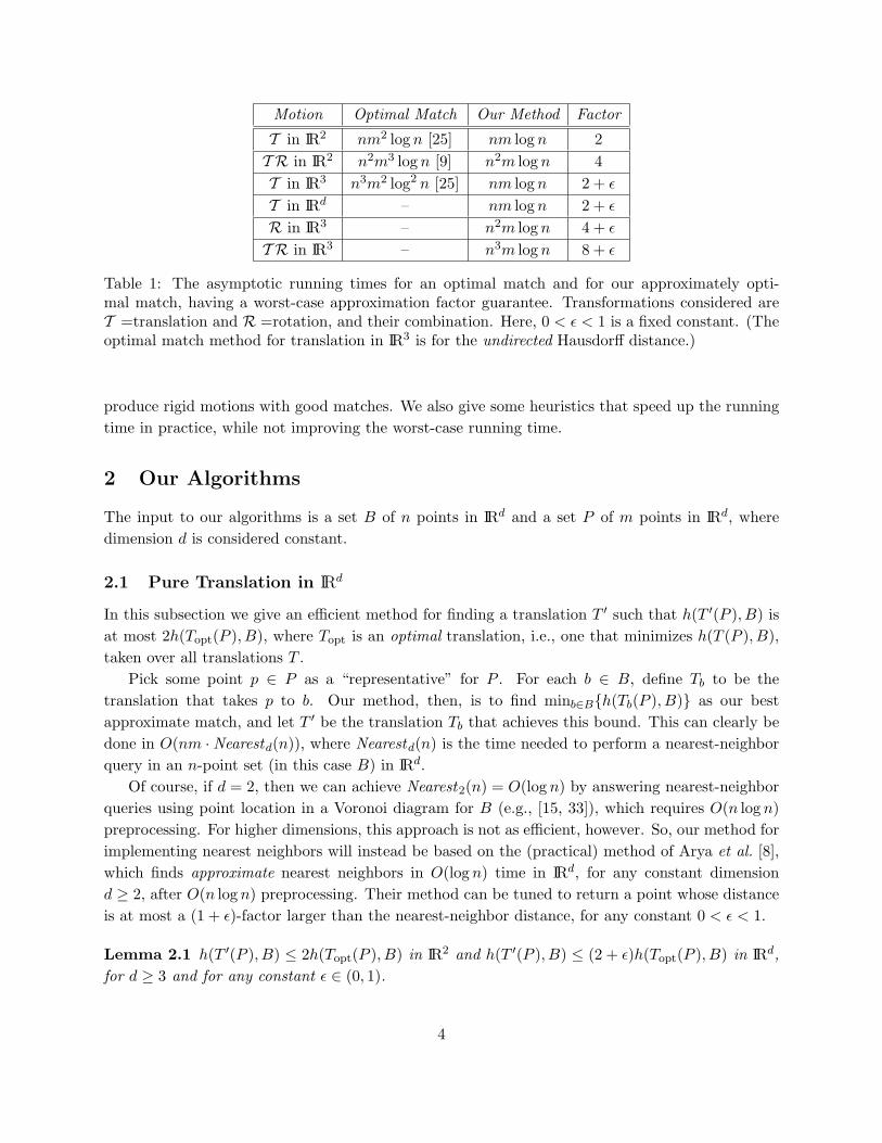
Motion Optimal Match Our Method Factor
T in IR2 nm2 log n [25] nm log n 2
T R in IR2 n2m3 log n [9] n2m log n 4
T in IR3 n3m2 log2 n [25] nm log n 2 + ǫ
T in IRd – nm log n 2 + ǫ
R in IR3 – n2m log n 4 + ǫ
T R in IR3 – n3m log n 8 + ǫ
Table 1: The asymptotic running times for an optimal match and for our approximately opti-mal match, having a worst-case approximation factor guarantee. Transformations considered areT =translation and R =rotation, and their combination. Here, 0 < ǫ < 1 is a fixed constant. (Theoptimal match method for translation in IR3 is for the undirected Hausdorff distance.)
produce rigid motions with good matches. We also give some heuristics that speed up the running
time in practice, while not improving the worst-case running time.
2 Our Algorithms
The input to our algorithms is a set B of n points in IRd and a set P of m points in IRd, where
dimension d is considered constant.
2.1 Pure Translation in IRd
In this subsection we give an efficient method for finding a translation T ′ such that h(T ′(P ), B) is
at most 2h(Topt(P ), B), where Topt is an optimal translation, i.e., one that minimizes h(T (P ), B),
taken over all translations T .
Pick some point p ∈ P as a “representative” for P . For each b ∈ B, define Tb to be the
translation that takes p to b. Our method, then, is to find minb∈B{h(Tb(P ), B)} as our best
approximate match, and let T ′ be the translation Tb that achieves this bound. This can clearly be
done in O(nm · Nearestd(n)), where Nearestd(n) is the time needed to perform a nearest-neighbor
query in an n-point set (in this case B) in IRd.
Of course, if d = 2, then we can achieve Nearest2(n) = O(log n) by answering nearest-neighbor
queries using point location in a Voronoi diagram for B (e.g., [15, 33]), which requires O(n log n)
preprocessing. For higher dimensions, this approach is not as efficient, however. So, our method for
implementing nearest neighbors will instead be based on the (practical) method of Arya et al. [8],
which finds approximate nearest neighbors in O(log n) time in IRd, for any constant dimension
d ≥ 2, after O(n log n) preprocessing. Their method can be tuned to return a point whose distance
is at most a (1 + ǫ)-factor larger than the nearest-neighbor distance, for any constant 0 < ǫ < 1.
Lemma 2.1 h(T ′(P ), B) ≤ 2h(Topt(P ), B) in IR2 and h(T ′(P ), B) ≤ (2 + ǫ)h(Topt(P ), B) in IRd,
for d ≥ 3 and for any constant ǫ ∈ (0, 1).
4
Proof: (For IR2) For simplicity of expression, define hopt = h(Topt(P ), B). Observe that for each
p ∈ Topt(P ), there exists an associated b ∈ B that is within a distance hopt of p. Consider the
process of translating the entire pattern Topt(P ) so that a particular point p now coincides with
its associated background point b. This translation will cover a distance of at most hopt and will
therefore increase the distance from any other point in the pattern to its associated background
point by at most hopt. Therefore, it will have a directed Hausdorff distance of at most twice that of
Topt(P ). This translation will be one of those generated and checked by our algorithm. Thus, our
algorithm will produce a translation that results in a directed Hausdorff distance that is at most a
factor of two times the minimal.
(For IRd) For the case of IRd, with d ≥ 3, an identical argument would apply if we were to use
an exact nearest-neighbor algorithm to compute the quality of the various translations considered.
However, we are using the approximate nearest-neighbor algorithm of Arya et al. [8], so the observed
directed Hausdorff distance of any translation T (P ) may appear to be greater (worse) than its
actual value by a factor of up to 1+ ǫ′, where ǫ′ is a parameter of the approximate nearest neighbor
algorithm. Since one of the candidate translations will have a directed Hausdorff distance within
a factor of 2 of the absolute optimal (by the argument above), our algorithm will select as the
best translation one that has a directed Hausdorff distance no greater than 2(1 + ǫ′)hopt. Selecting
ǫ′ = ǫ/2 then gives the desired result.
2.2 Translation and Rotation in IR2
For points in the plane, we give an efficient method for finding a Euclidean motion (translation and
rotation) E′ such that h(E′(P ), B) is at most 4h(Eopt(P ), B), where Eopt is an optimal Euclidean
motion, i.e., one that minimizes h(E(P ), B), taken over all valid motions E.
Select from the pattern diametrically opposing points and call them r and k; this can be
done trivially in time O(m2), but O(m log m) suffices [33]. Point r is treated as both the distinct
representative of the pattern for the translation part of the transformation and it is treated as
the center of rotation for the rotation part of the transformation. Specifically, for each b ∈ B,
define Tb to be the translation that takes r to b. Also for a b′ ∈ B, b′ 6= b, define Rb′ to be the
rotation about r that makes r, b′, and k collinear. Let Eb,b′ be the Euclidean motion that is the
combination of Tb and Rb′ . Our method is to find minb,b′∈B{h(Eb,b′(P ), B)} as our best approximate
match, and let E′ be the Euclidean motion Eb,b′ that achieves this bound. This can be done in
O(n2m·Nearest3(n)) time, which is O(n2m log2 n) if one uses the best current point location method
for a 3-dimensional convex subdivision [18] to query nearest neighbors in a 3-dimensional Voronoi
diagram (e.g., see [15, 33]). Our preference, however, is to achieve a faster (and more practical)
O(n2m log n) time bound using the approximate nearest neighbors method of Arya et al. [8], at a
slight cost in the approximation factor.
Lemma 2.2 h(E′(P ), B) ≤ (4 + ǫ)h(Eopt(P ), B), for any constant 0 < ǫ < 1.
Proof: Since the ǫ term is a direct consequence of our using approximate nearest neighbor
searching to achieve Nearest3(n) = O(log n), it is sufficient to show that actual nearest neighbors
5
would give an approximation factor of 4. For simplicity of expression, define hopt = h(Eopt(P ), B).
Observe that for each p ∈ Eopt(P ), there exists an associated b ∈ B that is within a distance hopt of
p. Consider the process of translating the entire pattern Eopt(P ) so that the particular point r now
coincides with its associated background point b. This translation will cover a distance of at most
hopt and will therefore increase the distance from any other point in the pattern to its associated
background point by at most hopt. Now consider the process of rotating the entire pattern about
point r so that the line containing r and k now passes through the background point associated
with k in Eopt(P ). This rotation will have the effect of moving point k by at most 2hopt. Since k is
the furthest point in the pattern from the center of rotation, all other pattern points will be moved
by a distance of at most 2hopt. Thus, any given point in the pattern can be moved by at most
hopt during the translation and at most 2hopt during the rotation, and could have been initially at
most hopt away from its associated background point. Therefore, each point in the pattern will be
at most a distance of 4hopt from a background point. The pattern in its current position coincides
with one of the Euclidean transformations generated and checked by our algorithm.
2.3 Pure Rotation in IR3
For points in IR3, we give an efficient method for finding a (pure) rotation R′, about the origin,
such that h(R′(P ), B) is at most 4h(Ropt(P ), B), where Ropt(P ) is an optimal rotation, i.e., one
that minimizes h(R(P ), B), taken over all rotations R.
Find a point p1 ∈ P that is furthest from the origin. Find a point p2 ∈ P that has the maximum
perpendicular distance to the line defined by the origin and point p1. (It takes O(m) time to find p1
and p2.) For each b′ ∈ B, define R1b′ to be the rotation that makes the origin, p1 and b′ collinear.
For each b′′ ∈ B, b′′ 6= b′, define R2b′′ to be the rotation about the origin-p1 axis that makes the
origin, p1, p2, and b′′ coplanar. Our method, then, is to find minb′,b′′∈B{h(R2b′′(R1b′(P )), B)} as
our best approximate match, and let R′ be the resultant rotation R2b′′(R1b′(P )) that achieves this
bound. This requires O(n2m · Nearest3(n)) time. As above, we achieve Nearest3(n) = O(log n)
using approximate nearest-neighbor searching [8], and end up with the following result:
Lemma 2.3 h(R′(P ), B) ≤ (4 + ǫ)h(Ropt(P ), B), for any constant 0 < ǫ < 1.
Proof: For simplicity of expression, define hopt = h(Ropt(P ), B). Observe that for each p ∈
Ropt(P ), there exists an associated b ∈ B that is within a distance hopt of p. Consider the process
of rotating the entire pattern Ropt(P ) so that p1, the furthest pattern point from the origin, now
becomes collinear with its associated background point b and the origin. This process can move
any point in the pattern by at most hopt. Now consider the second rotation (about the line through
the origin and p1) that brings p2 coplanar with its matching background point. This rotation may
move p2 a distance of at most 2hopt, and therefore it may move any point in the pattern by at
most 2hopt. These combined rotations move any pattern point at most a distance of 3hopt from its
original position, which is known to be within a distance of hopt of a background point. Therefore,
each point in the pattern will be a distance of at most 4hopt away from a background point. This
rotation will be one of those generated and checked by our algorithm.
6
2.4 Translation and Rotation in IR3
For points in IR3, we give an efficient method for finding a Euclidean transformation E′ such that
h(E′(P ), B) is at most (8 + ǫ)h(Eopt(P ), B), where Eopt is an optimal Euclidean transformation,
i.e., one that minimizes h(E(P ), B), taken over all such transformations E.
Select from the pattern diametrically opposing points2 and call them r and k. Choose a point
l ∈ P such that the perpendicular distance from l to the line rk is maximum. For each b ∈ B,
define Tb to be the translation that takes pattern point r to b. For each b′ ∈ B, b′ 6= b, define R1b′
to be the rotation that causes r, k and b′ to become collinear. For each b′′ ∈ B, b′′ 6= b′, b′′ 6= b,
define R2b′′ to be the rotation about the rk axis that brings b′′ into the (r, k, l)-plane.
Our method, then, is to compute the value of minb,b′,b′′∈B{h(R2b′′(R1b′(Tb(P ))), B)} as our best
approximate match, and let E′ be the Euclidean transformation R2b′′(R1b′(Tb(P )) that achieves this
bound. This can be done in O(n3m·Nearest3(n)) time. As above, we achieve Nearest3(n) = O(log n)
using approximate nearest-neighbor searching [8], and end up with the following result:
Lemma 2.4 h(E′(P ), B) ≤ (8 + ǫ)h(Eopt(P ), B), for any constant 0 < ǫ < 1.
Proof: For simplicity of expression, define hopt = h(Eopt(P ), B). In addition, as in previous
proofs, we show that the expansion factor is 8 if one were to use actual nearest neighbors instead
of approximate nearest neighbors. Observe that for each p ∈ Eopt(P ), there exists an associated
b ∈ B that is within a distance hopt of p. Consider the process of translating the entire pattern
Eopt(P ) so that r becomes coincident with its associated background point. This process can move
any point in the pattern by a distance of at most hopt. Now consider the process of rotating the
entire pattern so that line rk passes through the background point that is associated with k. This
rotation can move any point in the pattern by at most 2hopt. Now consider a second rotation
that brings the background point associated with l into the (r, l, k)-plane. This rotation may move
pattern point p2 a distance of at most 4hopt, and therefore it may move any point in the pattern
by at most 4hopt. This rotation will be one of those generated and checked by our algorithm. The
translation may have moved any point a distance of at most hopt, the first rotation may have moved
any point a distance of at most 2hopt farther, and the second rotation may have moved any point
a distance of at most 4hopt still farther. Considering that any given pattern point may have been
a distance of hopt away from its associated background point to start with, no pattern point can
be farther than 8hopt from its associated background point.
3 Experimental Results
We have implemented our methods and conducted experiments comparing them with a method
that produces best matches to an arbitrary precision using a conventional branch-and-bound search
of a discretized configuration space. This conventional method seems to be the most practical pre-
vious best match procedure (we did not feel it was practically feasible to implement the previous
2While subquadratic algorithms exist for computing the diameter, we found it reasonable to use a simple O(m2)
algorithm as a preprocessing step since we only need to perform this calculation once for the entire algorithm.
7
intersection-based methods). As we show through our experimental results, however, this conven-
tional method is still quite slow compared to our method, and the matches it finds are not that
much better than the ones that our method finds.
Example Generation. The background points B are generated uniformly at random in the unit
d-cube. We then randomly select m points from B to be an unperturbed pattern. We obtain a
perturbed pattern, P , by perturbing each pattern point by a small amount (uniformly, in a ball of
radius δ), so that the pattern no longer identically resembles a subset of the background points.
3.1 Implementation of the Approximate Match Algorithms
Pure Translation in IRd. As described in Section 2.1, our approximate pattern matching algo-
rithm translates the pattern so that the distinct representative of the pattern coincides with each of
the n background points in succession. For each such translation, the directed Hausdorff distance
is calculated and compared with the best found so far. If the new directed Hausdorff distance is
smaller than the best found so far, the position of the pattern (i.e., the position of the distinct
representative) and this new best distance replace those recorded so far. After the pattern has
been translated to each of the background points, we output the best translation found (which is
guaranteed to be within factor two of optimal).
There are various possible heuristics one can apply, which do not improve the worst-case running
time, but which do improve the running time in practice. We use a condition that terminates the
while-loop early once it is known that a particular placement need not be further considered.
Observe that in the calculation of the directed Hausdorff distance, we are finding the maximum
amount by which a pattern point deviates from its nearest background point. As we determine
this quantity for each of the pattern points we have a current maximum at any given point in
the loop. If this current maximum ever exceeds the best directed Hausdorff distance found so
far, the placement that we are checking is known to be suboptimal and does not warrant further
consideration. We therefore terminate the while loop as soon the partial computation of the directed
Hausdorff distance exceeds the global best found so far.
Translation and Rotation in IR2. Diametrically opposing pattern points are chosen from the
convex hull (in O(m2) time, as a preprocessing step), one of which will serve both as the distinct
representative of the pattern and as the center of rotation. The algorithm then translates the pat-
tern so that the distinct representative coincides with each of the n background points in succession.
After each translation, the pattern is rotated about the current position of the distinct represen-
tative a total of n − 1 times so that after each rotation, the other antipodal point is aligned with
another one of the background points. We now have the pattern in one of the n(n − 1) positions
at which we check the directed Hausdorff distance. As with the translation-only case, we maintain
the best directed Hausdorff distance found so far and the position of the pattern that produced
it. If at any time one of the n(n − 1) placements has a directed Hausdorff distance that is better
than the best found so far, our records are updated to reflect this new best position and directed
Hausdorff distance. Again, we use an early loop-termination heuristic for speed.
8
Translation and Rotation in IR3. We select the distinct representative and the antipode of
the pattern, as we have done in IR2 above. In this case, we also select a third pattern point,
called the radial point, which has the property that it is the greatest distance away from the line
passing through the distinct representative and the antipode. Our approximate match algorithm
is comprised of three nested for-loops. The outer-most loop translates the pattern such that the
distinct representative of the pattern coincides with each of the n background points in succession.
The next loop chooses one of the remaining n − 1 background points and rotates the pattern
about the current position of the distinct representative so that the antipode becomes aligned
with this selected background point. The inner-most for-loop selects a third background point
from the remaining n − 2 and performs a second rotation of the pattern, this time about the line
passing through the current position of the distinct representative and the current position of the
antipode, to bring the plane defined by the distinct representative, the antipode, and the radial
point into a position that includes the background point chosen by this third for-loop. For each of
the n(n − 1)(n − 2) placements produced by the above described for-loops, the directed Hausdorff
distance of the placement is generated and the current best is kept. At the termination of our
algorithm, we output the best placement found.
3.2 Implementation of the Branch and Bound Algorithms
Pure Translation in IR2. The conventional method against which we compared our method is
a recursive algorithm. It receives a square defined by a center point and a side length. It then
“probes” the center of the square by translating the pattern so that the distinct representative of
the pattern is in the center of the square. For the pattern in this position, the directed Hausdorff
distance is calculated. If this distance is the best found so far, it is recorded along with the probe
point (center of square). The algorithm then recurses on each of the four quadrants. The recursion
is terminated when it reaches a predefined maximum depth or if it is certain that placement of the
distinct representative at any point in the square will not produce a directed Hausdorff distance
that is better than the best found so far. One observation that we can use to terminate a branch
of recursion early is that the directed Hausdorff distance can be decreased by an amount of at
most x when the pattern is translated by a distance of x. If the value of the directed Hausdorff
distance produced by probing the center of the square is so great relative to the best found so far
that placing the distinct representative at any point in the square is known to produce a directed
Hausdorff distance that does not beat the best found so far, we no longer need to search recursively
this square and we can terminate this branch of the recursion.
Translation and Rotation in IR2. The conventional method for translation and rotation in IR2
involves searching the three-dimensional configuration space in which the x and y positions of the
distinct representative of the pattern comprise two of the dimensions, and the angular position, θ,
of the pattern about the distinct representative comprises the third.
Translation and Rotation in IR3. The conventional method for Translation and Rotation in
IR3 is again the search of a configuration space, which is now 6-dimensional: three degrees of
9
freedom (x, y, and z) in placing the distinct representative of the pattern, and three rotational
degrees of freedom (two in locating the antipode, and one in orienting the pattern about the axis
line through the antipode).
3.3 Experiment 1: Comparison of Match Qualities
While we have proved upper bounds on the worst-case behavior of our approximation algorithms,
the goal of our first experiment is to see how close to optimal Hausdorff distance our method comes,
in practice.
Pure Translation in IR2. We have proved an upper bound of 2 on the ratio of the directed
Hausdorff distance of our approximation to the directed Hausdorff distance of the optimal match
under translation. It is our conjecture that for large sparse B’s and large sparse P ’s, the approximate
match algorithms will produce matches that are (1 + λ)hopt, where λ is the ratio of the expected
distance by which a point will be perturbed divided by the maximum distance by which a point
will be perturbed; for our perturbation strategy in IR2, this ratio will be λ =∫ 10 r 2πrdr
π12 = 2/3. Our
reasoning is as follows. If the pattern is large, it is likely that the absolute optimal placement of
the pattern with respect to the background will be such that quite a few pattern points will be
hopt away from the nearest background point. The approximate-match algorithm produces, with
high probability (especially, given the pattern-generation method used in these experiments), the
match that is identical to this optimal match, differing only in that it is translated such that the
distinct representative of the pattern is made to coincide with its associated background point. This
translation will be in a direction that moves one or more of the poorly matching pattern points
almost directly away from the associated background points. Thus, since λ = 23 , the expected
Hausdorff distance for our algorithm will be 53 · hopt.
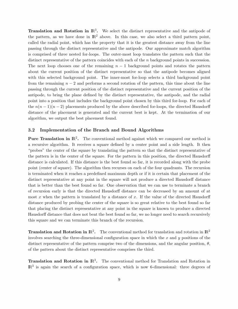
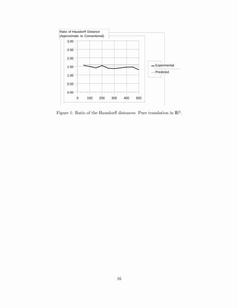
We conducted an experiment to test this hypothesis. One hundred sets of background points
were generated, each having between 50 and 500 points. From each background, a pattern of
size 10 was selected and perturbed. The pattern was then matched to its associated background
using both the approximate match algorithm and a conventional match algorithm. The ratio of
the directed Hausdorff distance of the match produced by the approximate match algorithm to the
directed Hausdorff distance of the match produced by the conventional match algorithm is plotted
in Figure 1. The average of the ratios plotted is 1.44, which is close to the predicted value of 1.66.
Note that the predicted value of this ratio assumes an infinitely large pattern and an unlimited
depth of recursion in the conventional method. Decreasing either the pattern size or the depth of
recursion would decrease the predicted value of the ratio and this too is reflected in this experiment.
For this experiment, the conventional match algorithm was run to a depth of eleven.
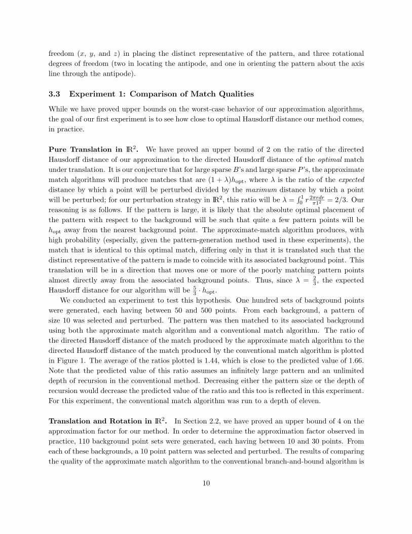
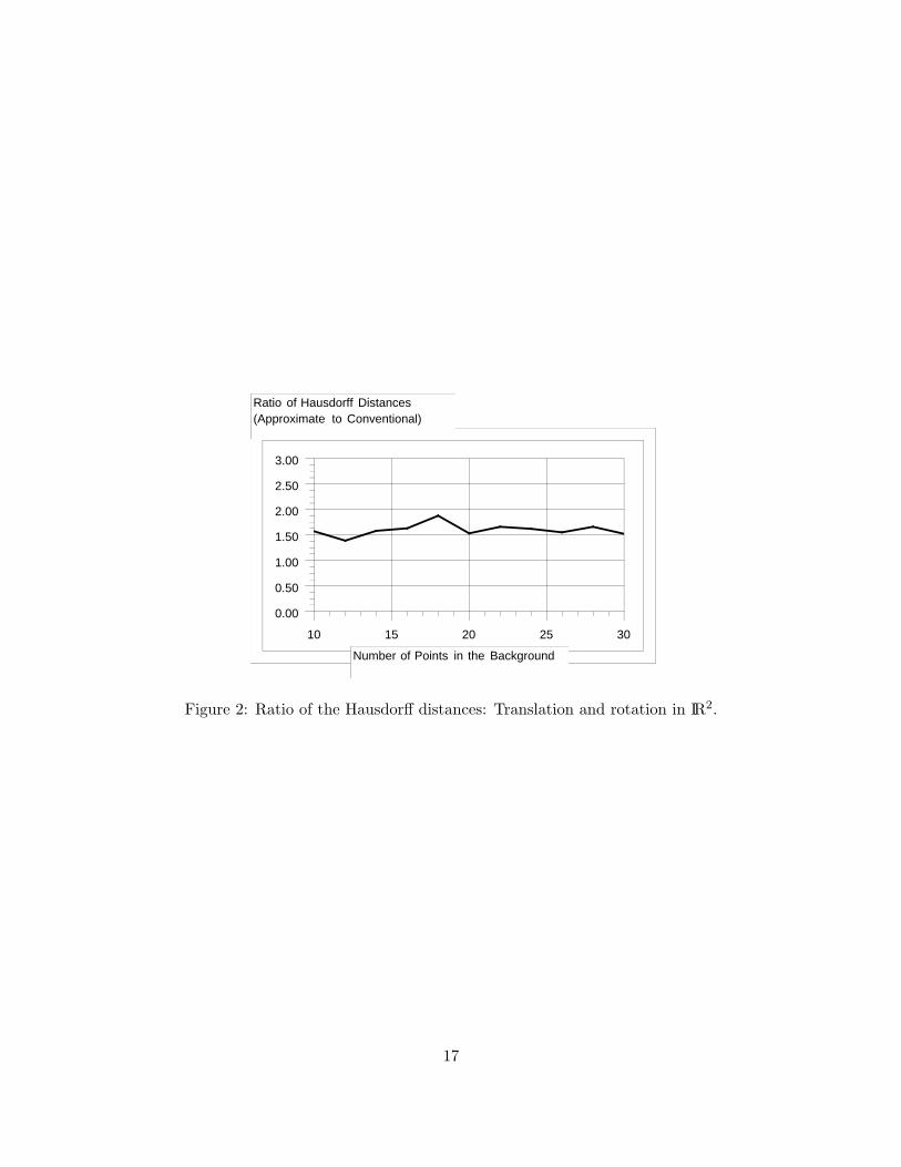
Translation and Rotation in IR2. In Section 2.2, we have proved an upper bound of 4 on the
approximation factor for our method. In order to determine the approximation factor observed in
practice, 110 background point sets were generated, each having between 10 and 30 points. From
each of these backgrounds, a 10 point pattern was selected and perturbed. The results of comparing
the quality of the approximate match algorithm to the conventional branch-and-bound algorithm is
10
plotted in Figure 2. The average ratio of the trials in this experiment is 1.60, which is substantially
better than the worst-case ratio of 4.
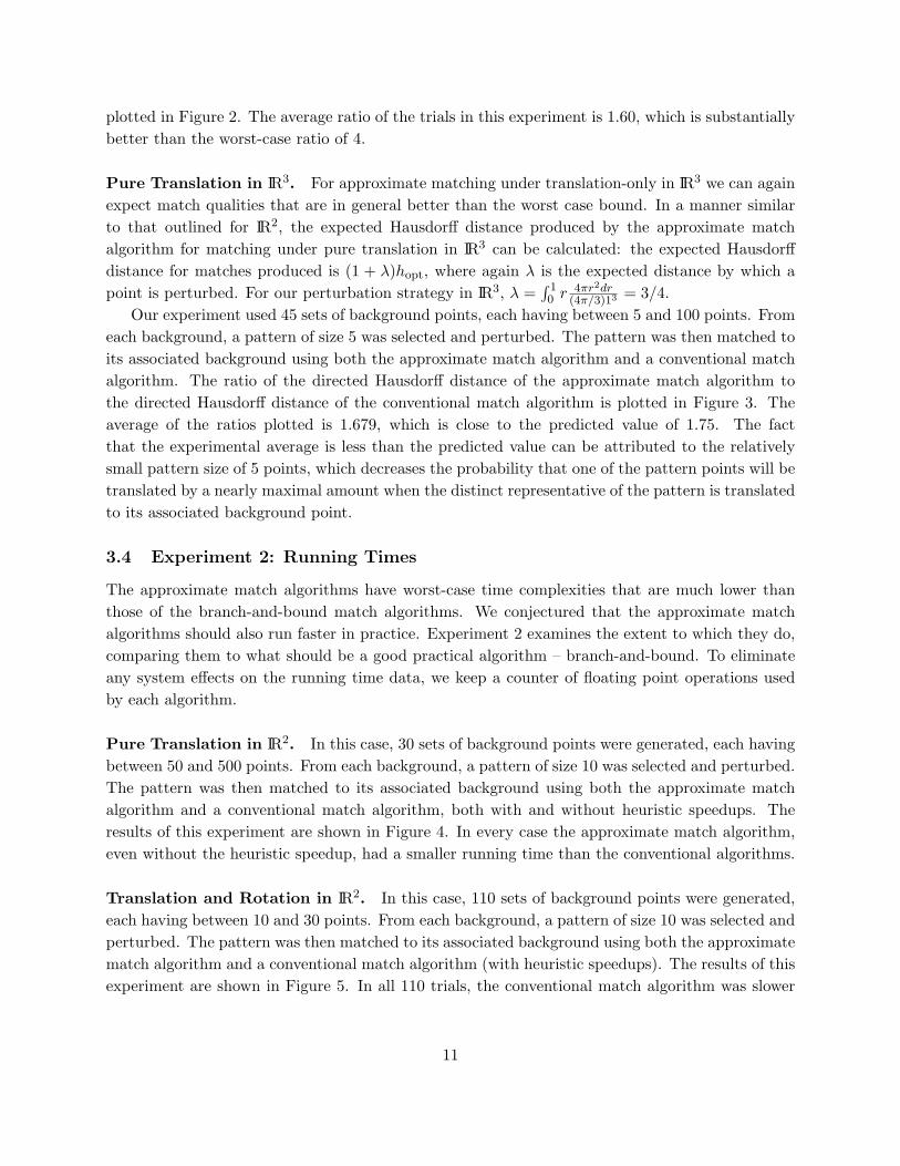
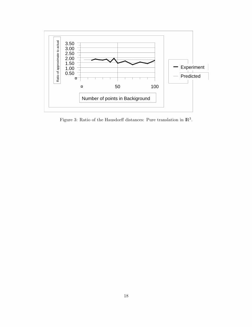
Pure Translation in IR3. For approximate matching under translation-only in IR3 we can again
expect match qualities that are in general better than the worst case bound. In a manner similar
to that outlined for IR2, the expected Hausdorff distance produced by the approximate match
algorithm for matching under pure translation in IR3 can be calculated: the expected Hausdorff
distance for matches produced is (1 + λ)hopt, where again λ is the expected distance by which a
point is perturbed. For our perturbation strategy in IR3, λ =∫ 10 r 4πr2dr
(4π/3)13 = 3/4.
Our experiment used 45 sets of background points, each having between 5 and 100 points. From
each background, a pattern of size 5 was selected and perturbed. The pattern was then matched to
its associated background using both the approximate match algorithm and a conventional match
algorithm. The ratio of the directed Hausdorff distance of the approximate match algorithm to
the directed Hausdorff distance of the conventional match algorithm is plotted in Figure 3. The
average of the ratios plotted is 1.679, which is close to the predicted value of 1.75. The fact
that the experimental average is less than the predicted value can be attributed to the relatively
small pattern size of 5 points, which decreases the probability that one of the pattern points will be
translated by a nearly maximal amount when the distinct representative of the pattern is translated
to its associated background point.
3.4 Experiment 2: Running Times
The approximate match algorithms have worst-case time complexities that are much lower than
those of the branch-and-bound match algorithms. We conjectured that the approximate match
algorithms should also run faster in practice. Experiment 2 examines the extent to which they do,
comparing them to what should be a good practical algorithm – branch-and-bound. To eliminate
any system effects on the running time data, we keep a counter of floating point operations used
by each algorithm.
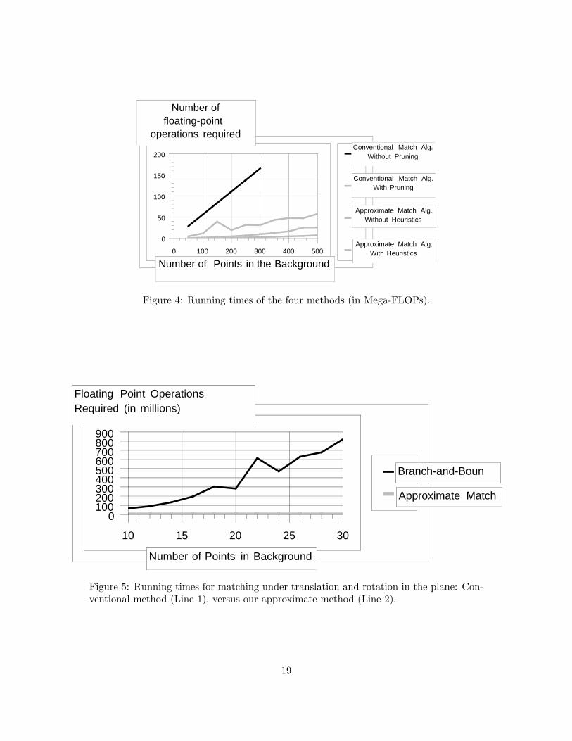
Pure Translation in IR2. In this case, 30 sets of background points were generated, each having
between 50 and 500 points. From each background, a pattern of size 10 was selected and perturbed.
The pattern was then matched to its associated background using both the approximate match
algorithm and a conventional match algorithm, both with and without heuristic speedups. The
results of this experiment are shown in Figure 4. In every case the approximate match algorithm,
even without the heuristic speedup, had a smaller running time than the conventional algorithms.
Translation and Rotation in IR2. In this case, 110 sets of background points were generated,
each having between 10 and 30 points. From each background, a pattern of size 10 was selected and
perturbed. The pattern was then matched to its associated background using both the approximate
match algorithm and a conventional match algorithm (with heuristic speedups). The results of this
experiment are shown in Figure 5. In all 110 trials, the conventional match algorithm was slower
11
than the approximate match algorithm by at least a factor of 442; the average slowdown being a
factor of 1199.
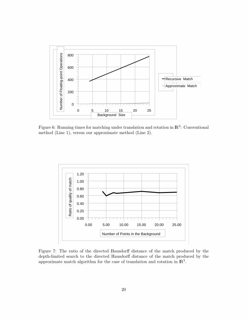
Translation and Rotation in IR3. In this case, 24 sets of background points were generated,
each having between 5 and 25 points. From each background, a pattern of size 5 was selected
and perturbed. The pattern was then matched to its associated background using the approximate
match algorithm with heuristic speedups, a depth-first branch-and-bound algorithm and a breadth-
first branch-and-bound algorithm. The running times of the depth-first and breadth-first branch-
and-bound algorithms were, in all instances within a factor of 0.01 of each other and are therefore
plotted as a single line in Figure 6, which depicts the results of this experiment.
The branch-and-bound algorithms search a six-dimensional space comprised of three degrees of
freedom in the translation of the pattern and three degrees of freedom in the rotation of the pattern.
This produces a rather large branching factor of 26 = 64 in the recursive algorithms, and necessi-
tated the depth of these algorithms to be limited to 3. With this (necessary) depth limitation, the
approximate-match algorithm actually found better matches than the branch-and-bound algorithm
did in all of the 24 cases, in spite of the fact that the branch-and-bound algorithms required on
average 4479 times as many floating-point operations. The ratio of the directed Hausdorff distance
of the match produced by the depth-limited search to the directed Hausdorff distance of the match
produced by the approximate match algorithm is plotted in Figure 7. It should be noted that the
largest of the breadth-first searches in this experiment consumed between one and two hours of real
time on an otherwise unloaded Sun Sparc Station ELC running Sun OS 4.1.1.
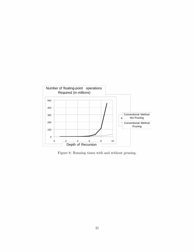
3.5 Experiment 3: Running Times vs. Depth of Recursion
The depth of search of the conventional match algorithms that we have implemented must be
limited. This experiment depicts the extent to which the running time of the algorithm increases
as the depth of recursion is increased. Further, it shows the substantial speedup obtained by
pruning the search. The results of this experiment are depicted in Figure 8.
Four backgrounds were generated, each having 50 points. From each background, a pattern of
size 10 was selected and perturbed. The conventional method with and without pruning was run
ten times on each of the four data sets with the depth of recursion being varied from 1 to 10. An
average of the running times of each of the four cases was taken and the results were plotted in
Figure 8.
4 Discussion and Conclusion
We have given approximate pattern matching algorithms for translation, rotation, and Euclidean
transformations for point sets in two or more dimensions. Our algorithms are guaranteed to give a
match with a directed Hausdorff distance that is no greater than a small constant times the best
achievable directed Hausdorff distance. In addition, they have a time complexity that is substan-
tially smaller than those of existing pattern matching algorithms, they are easy to implement, and
they run fast in practice.
12
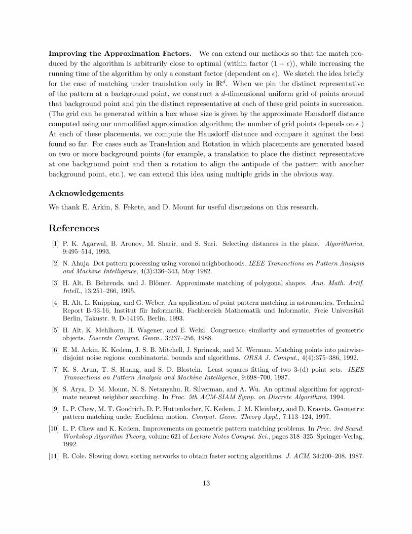
Improving the Approximation Factors. We can extend our methods so that the match pro-
duced by the algorithm is arbitrarily close to optimal (within factor (1 + ǫ)), while increasing the
running time of the algorithm by only a constant factor (dependent on ǫ). We sketch the idea briefly
for the case of matching under translation only in IRd. When we pin the distinct representative
of the pattern at a background point, we construct a d-dimensional uniform grid of points around
that background point and pin the distinct representative at each of these grid points in succession.
(The grid can be generated within a box whose size is given by the approximate Hausdorff distance
computed using our unmodified approximation algorithm; the number of grid points depends on ǫ.)
At each of these placements, we compute the Hausdorff distance and compare it against the best
found so far. For cases such as Translation and Rotation in which placements are generated based
on two or more background points (for example, a translation to place the distinct representative
at one background point and then a rotation to align the antipode of the pattern with another
background point, etc.), we can extend this idea using multiple grids in the obvious way.
Acknowledgements
We thank E. Arkin, S. Fekete, and D. Mount for useful discussions on this research.
References
[1] P. K. Agarwal, B. Aronov, M. Sharir, and S. Suri. Selecting distances in the plane. Algorithmica,9:495–514, 1993.
[2] N. Ahuja. Dot pattern processing using voronoi neighborhoods. IEEE Transactions on Pattern Analysis
and Machine Intelligence, 4(3):336–343, May 1982.
[3] H. Alt, B. Behrends, and J. Blomer. Approximate matching of polygonal shapes. Ann. Math. Artif.
Intell., 13:251–266, 1995.
[4] H. Alt, L. Knipping, and G. Weber. An application of point pattern matching in astronautics. TechnicalReport B-93-16, Institut fur Informatik, Fachbereich Mathematik und Informatic, Freie UniversitatBerlin, Takustr. 9, D-14195, Berlin, 1993.
[5] H. Alt, K. Mehlhorn, H. Wagener, and E. Welzl. Congruence, similarity and symmetries of geometricobjects. Discrete Comput. Geom., 3:237–256, 1988.
[6] E. M. Arkin, K. Kedem, J. S. B. Mitchell, J. Sprinzak, and M. Werman. Matching points into pairwise-disjoint noise regions: combinatorial bounds and algorithms. ORSA J. Comput., 4(4):375–386, 1992.
[7] K. S. Arun, T. S. Huang, and S. D. Blostein. Least squares fitting of two 3-(d) point sets. IEEE
Transactions on Pattern Analysis and Machine Intelligence, 9:698–700, 1987.
[8] S. Arya, D. M. Mount, N. S. Netanyahu, R. Silverman, and A. Wu. An optimal algorithm for approxi-mate nearest neighbor searching. In Proc. 5th ACM-SIAM Symp. on Discrete Algorithms, 1994.
[9] L. P. Chew, M. T. Goodrich, D. P. Huttenlocher, K. Kedem, J. M. Kleinberg, and D. Kravets. Geometricpattern matching under Euclidean motion. Comput. Geom. Theory Appl., 7:113–124, 1997.
[10] L. P. Chew and K. Kedem. Improvements on geometric pattern matching problems. In Proc. 3rd Scand.
Workshop Algorithm Theory, volume 621 of Lecture Notes Comput. Sci., pages 318–325. Springer-Verlag,1992.
[11] R. Cole. Slowing down sorting networks to obtain faster sorting algorithms. J. ACM, 34:200–208, 1987.
13
[12] R. Cole. Parallel merge sort. SIAM J. Comput., 17(4):770–785, 1988.
[13] R. Cole, J. Salowe, W. Steiger, and E. Szemeredi. An optimal-time algorithm for slope selection. SIAM
J. Comput., 18:792–810, 1989.
[14] T. H. Cormen, C. E. Leiserson, and R. L. Rivest. Introduction to Algorithms. MIT Press, Cambridge,MA, 1990.
[15] H. Edelsbrunner. Algorithms in Combinatorial Geometry, volume 10 of EATCS Monographs on Theo-
retical Computer Science. Springer-Verlag, Heidelberg, West Germany, 1987.
[16] D. Forsyth, J. L. Mundy, A. Zisserman, C. Coelho, A. Heller, and C. Rothwell. Invariant descriptorsfor 3-d object recognition and pose. IEEE Transactions on Pattern Analysis and Machine Intelligence,13(10):971–991, 1991.
[17] J. W. Foster, G. K. Bennett, and P. M. Griffin. Automated visual inspection: Quality control techniquesfor the modern manufacturing environment. Proceedings of 1987 IIE Integrated Systems Conference,pages 135–140, Dec. 1987.
[18] M. T. Goodrich and R. Tamassia. Dynamic trees and dynamic point location. SIAM J. Comput., 28(2),1999, 612–636.
[19] P. M. Griffin, J. W. Foster, and M. H. Han. Automated dimension verification by point pattern matching.Proceedings of 1988 International Industrial Engineering Conference, pages 451–455, 1988.
[20] R. M. Haralick, C. N. Lee, X. Zhuang, V. G. Vaidya, and M. B. Kim. Pose estimation from correspondingpoint data. IEEE Transactions on Systems, Man and Cybernetics, 19(6):1426–1446, Nov.-Dec. 1989.
[21] P. J. Heffernan. Generalized approximate algorithms for point set congruence. In Proc. 3rd Workshop
Algorithms Data Struct., volume 709 of Lecture Notes Comput. Sci., pages 373–384. Springer-Verlag,1993.
[22] P. J. Heffernan and S. Schirra. Approximate decision algorithms for point set congruence. Comput.
Geom. Theory Appl., 4:137–156, 1994.
[23] B. K. P. Horn. Closed-form solution of absolute orientation using unit quaternions. Journal of the
Optical Society of America A, 4(4):629–642, Apr. 1987.
[24] B. K. P. Horn, H. M. Hilden, and S. Negahdaripour. Closed-form solution of absolute orientation usingorthonormal matrices. Journal of the Optical Society of America A, 5(7):1127–1135, July 1988.
[25] D. P. Huttenlocher, K. Kedem, and J. M. Kleinberg. On dynamic Voronoi diagrams and the minimumHausdorff distance for point sets under Euclidean motion in the plane. In Proc. 8th Annu. ACM Sympos.
Comput. Geom., pages 110–120, 1992.
[26] D. P. Huttenlocher, K. Kedem, and M. Sharir. The upper envelope of Voronoi surfaces and its applica-tions. Discrete Comput. Geom., 9:267–291, 1993.
[27] K. Imai, S. Sumino, and H. Imai. Minimax geometric fitting of two corresponding sets of points. InProc. 5th Annu. ACM Sympos. Comput. Geom., pages 266–275, 1989.
[28] D. J. Kahl, A. Rosenfeld, and A. Danker. Some experiments in point pattern matching. IEEE Trans-
actions on Systems, Man and Cybernetics, 10(2):105–116, 1980.
[29] L. J. Kitchen. Relaxation for point-pattern matching: What it really computes. IEEE CVPR, pages405–407, 1985.
[30] N. Megiddo. Applying parallel computation algorithms in the design of serial algorithms. J. ACM,30:852–865, 1983.
[31] H. Ogawa. Labeled point pattern matching by fuzzy relaxation. Pattern Recognition, 17(5):569–573,1984.
14
[32] H. Ogawa. Labeled point pattern matching by delaunay trangulation and maximal cliques. Pattern
Recognition, 19(1):35–40, 1986.
[33] F. P. Preparata and M. I. Shamos. Computational Geometry: An Introduction. Springer-Verlag, NewYork, NY, 1985.
[34] S. Ranade and A. Rosenfeld. Point pattern matching by relaxation. Pattern Recognition, 12:269–275,1980.
[35] W. Rucklidge. Lower bounds for the complexity of the Hausdorff distance. In Proc. 5th Canad. Conf.
Comput. Geom., pages 145–150, 1993.
[36] G. Stockman, S. Kopstein, and S. Benett. Matching images to models for registration and objectdetection via clustering. IEEE Transactions on Pattern Analysis and Machine Intelligence, 4(3):229–241, May 1982.
[37] S. Umeyama. Least-squares estimation of transformation parameters between two point patterns. IEEE
Transactions on Pattern Analysis and Machine Intelligence., 13(4):376–380, Apr. 1991.
[38] C. Wang, H. Sun, S. Yada, and A. Rosenfeld. Some experiments in relaxation image matching usingcorner features. Pattern Recognition, 16(2):167–182, 1983.
15
1
2
0 100 200 300 400 500
0.00
0.50
1.00
1.50
2.00
2.50
3.00
Ratio of Hausdorff Distance(Approximate to Conventional)
Experimental
Predicted
Figure 1: Ratio of the Hausdorff distances: Pure translation in IR2.
16
10 15 20 25 30
0.00
0.50
1.00
1.50
2.00
2.50
3.00
Ratio of Hausdorff Distances(Approximate to Conventional)
Number of Points in the Background
Figure 2: Ratio of the Hausdorff distances: Translation and rotation in IR2.
17
1
2
Number of points in Backiground
¤ 50 100
Rat
io o
f app
roxi
mat
e to
act
ual
¤0.501.001.502.002.503.003.50
Experiment
Predicted
Figure 3: Ratio of the Hausdorff distances: Pure translation in IR3.
18
1
2
3
40 100 200 300 400 500
0
50
100
150
200Conventional Match Alg.
Without Pruning
Number offloating-point
operations required
Conventional Match Alg.With Pruning
Approximate Match Alg.Without Heuristics
Approximate Match Alg.With Heuristics
Number of Points in the Background
Figure 4: Running times of the four methods (in Mega-FLOPs).
1
2
10 15 20 25 30
0100200300400500600700800900
Number of Points in Background
Floating Point OperationsRequired (in millions)
Approximate Match
Branch-and-Boun
Figure 5: Running times for matching under translation and rotation in the plane: Con-ventional method (Line 1), versus our approximate method (Line 2).
19
1
2
0 5 10 15 20 25Num
ber
of F
loat
ing-
poin
t Ope
ratio
ns
0
200
400
600
800
Approximate Match
Recursive Match
Background Size
Figure 6: Running times for matching under translation and rotation in IR3: Conventionalmethod (Line 1), versus our approximate method (Line 2).
Number of Points in the Background
0.00 5.00 10.00 15.00 20.00 25.00
Rat
io o
f qua
lity
of m
atch
0.00
0.20
0.40
0.60
0.80
1.00
1.20
Figure 7: The ratio of the directed Hausdorff distance of the match produced by thedepth-limited search to the directed Hausdorff distance of the match produced by theapproximate match algorithm for the case of translation and rotation in IR3.
20
1
2
0 2 4 6 8 10
0
100
200
300
400
500
Depth of Recursion
Number of floating-point operationsRequired (in millions)
Conventional MethodNO Pruning
Conventional MethodPruning
Figure 8: Running times with and without pruning.
21
Recommended