Confidence bands for a log-concave density
Guenther Walther*1, Alnur Ali1,2, Xinyue Shen2,3, and Stephen Boyd2
1Department of Statistics, Stanford University2Department of Electrical Engineering, Stanford University
3Shenzhen Research Institute of Big Data and Future Network of Intelligence Institute, ChineseUniversity of Hong Kong
{gwalther,alnurali,xinyues,boyd}@stanford.edu
revised November 2021
Abstract
We present a new approach for inference about a univariate log-concave distribution: Instead of usingthe method of maximum likelihood, we propose to incorporate the log-concavity constraint in an appropriatenonparametric confidence set for the cdf F . This approach has the advantage that it automatically providesa measure of statistical uncertainty and it thus overcomes a marked limitation of the maximum likelihoodestimate. In particular, we show how to construct confidence bands for the density that have a finite sampleguaranteed confidence level. The nonparametric confidence set for F which we introduce here has attractivecomputational and statistical properties: It allows to bring modern tools from optimization to bear on thisproblem via difference of convex programming, and it results in optimal statistical inference. We show thatthe width of the resulting confidence bands converges at nearly the parametric n−
12 rate when the log density
is k-affine.
1 Introduction
Statistical inference under shape constraints has been the subject of continued considerable research activity.Imposing shape constraints on the inference about a function f , that is, assuming that the function satisfiescertain qualitative properties, such as monotonicity or convexity on certain subsets of its domain, has two mainmotivations: First, such shape constraints may directly arise from the problem under investigation and it is thendesirable that the result of the inference reflects this fact. The second reason is that alternative nonparametricestimators typically involve the choice of a tuning parameter, such as the bandwidth in the case of a kernelestimator. A good choice for such a tuning parameter is usually far from trivial. More importantly, selecting atuning parameter injects a certain amount of subjectivity into the estimator, and the resulting choice may provequite consequential for relevant aspects of the inference. In contrast, imposing shape constraints often allows toderive an estimator that does not depend on a tuning parameter while at the same time exhibiting a good statisticalperformance, such as achieving optimal minimax rates of convergence to the underlying function f .
*Research supported by NSF grants DMS-1501767 and DMS-1916074
1
arX
iv:2
011.
0366
8v2
[m
ath.
ST]
26
Nov
202
1
This paper is concerned with inference about a univariate log-concave density, i.e. a density of the form
f(x) = expφ(x),
where φ : R → [–∞,∞) is a concave function. It was argued in Walther (2002) that log-concave densitiesrepresent an attractive and useful nonparametric surrogate for the class of Gaussian distributions for a range ofproblems in inference and modeling. The appealing properties of this class are that it contains most commonlyencountered parametric families of unimodal densities with exponentially decaying tails and that the class isclosed under convolution, affine transformations, convergence in distribution and marginalization. In a similarvein as a normal distribution can be seen as a prototypical model for a homogenous population, one can use theclass of log-concave densities as a more flexible nonparametric model for this task, from which heterogenousmodels can then be built e.g. via location mixtures. Historically such homogenous distributions have beenmodeled with unimodal densities, but it is known that the maximum likelihood estimate (MLE) of a unimodaldensity does not exist, see e.g. Birge (1997). In contrast, it was shown in Walther (2002) that the MLE of alog-concave density exists and can be computed with readily available algorithms. Therefore, the class of log-concave densities is a sufficiently rich nonparametric model while at the same time it is small enough to allownonparametric inference without a tuning parameter.
Due to these attractive properties there has been a considerable research activity in the last 15 years aboutthe statistical properties of the MLE, computational aspects, applications in modeling and inference, and themultivariate setting. Many of the key properties of the MLE are now well understood: Existence of the MLEwas shown in Walther (2002), consistency was proved by Pal, Woodroofe and Meyer (2007), and rates of con-vergence in certain uniform metrics was established by Dumbgen and Rufibach (2009). Balabdaoui, Rufibachand Wellner (2009) provided pointwise limit distributribution theory, while Doss and Wellner (2016) and Kimand Samworth (2016) gave rates rates of convergence in the Hellinger metric, and Kim, Guntuboyina and Sam-worth (2018) proved adaptation properties. Accompanying results for the multivariate case are given in e.g.Cule, Samworth and Stewart (2010), Schuhmacher and Dumbgen (2010), Seregin and Wellner (2010), Kim andSamworth (2016), and Feng, Guntuboyina, Kim and Samworth (2020).
Computation of the univariate MLE was initially approached with the Iterative Convex Minorant Algorithm,see Walther (2002), Pal, Woodroofe and Meyer (2007) and Rufibach (2007), but it appears that the fastest algo-rithms currently available are the active set algorithm given in Dumbgen, Husler and Rufibach (2007) and theconstrained Newton method proposed by Liu and Wang (2018).
Overviews of some of these results and other work involving modeling and inference with log-concave dis-tributions are given in the review papers of Walther (2009), Saumard and Wellner (2014) and Samworth (2018).
Notably, the existing methodology for estimating a log-concave density appears to be exclusively focused onthe method of maximum likelihood. Here we will employ a different methodology: We will derive a confidenceband by intersecting the log-concavity constraint with a goodness-of-fit test. One important advantage of thisapproach is that such a confidence band satisfies a key principle of statistical inference: an estimate needs tobe accompanied by some measure of standard error in order to be useful for inference. There appears to beno known method for obtaining such a confidence band via the maximum likelihood approach. Balabdaoui etal. (2009) construct pointwise confidence intervals for a log-concave density based on asymptotic limit theory,which requires to estimate the second derivative of log f(x). Azadbakhsh et al. (2014) compare several methodsfor estimating this nuisance parameter and they report that this task is quite difficult. An alternative approachis given by Deng et al. (2020). In Section 5 we compare the confidence bands introduced here with pointwiseconfidence intervals obtained via the asymptotic limit theory as well as with the bootstrap. Of course, pointwise
2
confidence intervals have a different goal than confidence bands. The pointwise intervals will be be shorterbut the the confidence level will not hold simultaneously across multiple locations. In contrast, the method weintroduce here comes with strong guarantees in terms of finite sample valid coverage levels across locations.
2 Constructing a confidence band for a log-concave density
Given data X1, . . . , Xn from a log-concave density f we want to find functions ˆ(x) = ˆ(x,X1, . . . , Xn) andµ(x) = µ(x,X1, . . . , Xn) such that
IPf
{ˆ(x) ≤ f(x) ≤ µ(x) for all x ∈ R
}≥ 1− α
for a given confidence level 1− α ∈ (0, 1). It is well known that in the case of a general density f no non-trivialconfidence interval (ˆ(x), µ(x)) exists, see e.g. Donoho (1988). However, assuming a shape-constraint for fsuch as log-concavity allows to construct pointwise and uniform confidence statements as follows:
Let Cn(α) be a 1− α confidence set for the distribution function F of f , i.e.
IPF {F ∈ Cn(α)} ≥ 1− α. (1)
Such a nonparametric confidence set always exists, e.g. the Kolmogorov-Smirnov bands give a confidence setfor F (albeit a non-optimal one). Define
ˆ(x) := inff is log-concave and F∈Cn(α)
f(x) (2)
and define µ(x) analogously with sup in place of inf. If f is log-concave then (1) and (2) imply
IPf
{ˆ(x) ≤ f(x) ≤ µ(x)
}≥ 1− α,
so we obtain a 1−α confidence interval for f(x) by solving the optimization problem (2). Moreover, if we solve(2) at multiple locations x1, . . . , xm, then we obtain
IPf
{ˆ(xi) ≤ f(xi) ≤ µ(xi) for all i = 1, . . . ,m
}≥ 1− α. (3)
So the coverage probability is automatically simultaneous across multiple locations and comes with a finitesample guarantee, since it is inherited from the confidence set Cn in (1). Likewise, the quality of the confidenceband, as measured e.g. by the width µ(x)− ˆ(x), will also derive from Cn, which therefore plays a central role inthis approach. Finally, the log-concavity constraint allows to extend the confidence set (3) to a confidence bandon the real line, as we will show in Section 2.4.
Hengartner and Stark (1995), Dumbgen (1998), Dumbgen (2003) and Davies and Kovac (2004) employ theabove approach for inference about a unimodal or a k-modal density. Here we introduce a new confidence setCn(α) for F . This confidence set is adapted from methodology developed in the abstract Gaussian White Noisemodel by Walther and Perry (2019) for optimal inference in settings related to the one considered here. Thereforethis confidence set should also prove useful for the works about inference in the unimodal and k-modal settingcited above.
The key conceptual problem for solving the optimization problem (2) is that f is infinite dimensional. We
3
will overcome this by using the log-concavity of f to relax Cn(α) to a finite dimensional superset, which makesit possible to compute (2) with fast optimization algorithms. We will address these tasks in turn in the followingsubsections.
2.1 A confidence set for F
Given X1, . . . , Xn i.i.d. from the continuous cdf F we set sn := dlog2 log ne and
xi := X(1+(i−1)2sn ), i = 1, . . . ,m :=
⌊n− 1
2sn
⌋+ 1, (4)
where X(j) denotes the jth order statistic. Our analysis will use only the subset {xi} of the data, i.e. the setcontaining every log n th order statistic; see Remark 3 for why this is sufficient.
Translating the methodology of the ‘Bonferroni scan’ developed in Walther and Perry (2019) from the Gaus-sian White Noise model to the density setting suggests employing a confidence set of the form
Cn(α) :=
{F : cjkB ≤ F (xk)− F (xj) ≤ djkB for all (j, k) ∈ I =
⋃B
IB
}.
with cjkB, djkB, I given below. The idea is to choose an index set I that is rich enough to detect relevantdeviations from the empirical distribution, but which is also sparse enough so that the |I| constraints can becombined with a simple weighted Bonferroni adjustment and still result in optimal inference. The second keyingredient of this construction is to let the weights of the Bonferroni adjustment depend on j− i in a certain way.See Walther and Perry (2019) for a comparison of the finite sample and asymptotic performance of this approachwith other relevant calibrations, such as the ones used in the works cited above.
Note that the confidence set Cn(α) checks the probability content of random intervals (xj , xk), which au-tomatically adapt to the empirical distribution. This makes it possible to detect relevant deviations from theempirical distribution with a relatively small number of such intervals, which is key for making the Bonferroniadjustment powerful as well as for efficient computation. Moreover, using such random intervals makes thebounds cjkB, djkB distribution-free since F (xk)− F (xj) ∼ Beta((k− j)2sn , n+ 1− (k− j)2sn), see Ch. 3.1in Shorack and Wellner (1986).
The precise specifications of cjkB, djkB, I are as follows:
I :=
Bmax⋃B=0
IB, where Bmax := blog2n8 c − sn
IB :={
(j, k) : j = 1 + (i− 1)2B, k = 1 + i2B for i = 1, . . . , nB :=⌊ n− 1
2B+sn
⌋}cjkB := cB := qBeta
( α
2(B + 2)nBtn, 2B+sn , n+ 1− 2B+sn
)djkB := dB := qBeta
(1− α
2(B + 2)nBtn, 2B+sn , n+ 1− 2B+sn
)where tn :=
∑BmaxB=0
1B+2 and qBeta (α, r, s) denotes the α-quantile of the beta distribution with parameters
r and s. The term 1B+2 is a weighting factor in the Bonferroni adjustment which results in an advantageous
statistical performance, see Walther and Perry (2019). It follows from the union bound that IPF (F ∈ Cn(α)) ≥
4
1− α whenever F is continuous.Remarks: 1. An alternative way to control the distribution of F (xk) − F (xj) is via a log-likelihood ra-
tio type transformation and Hoeffding’s inequality, see Rivera and Walther (2013) and Li, Munk, Sieling andWalther (2020). This results in a loss of power due to the slack in Hoeffding’s inequality and the slack frominverting the log-likelihood ratio transformation with an inequality. Simulations show that the above approachusing an exact beta distribution is less conservative despite the use of Bonferroni’s inequality to combine thestatistics across I.
2. The inference is based on the statistic F ((xj , xk)), i.e. the unknown F evaluated on the random interval(xj , xk), rather than on the more commonly used statistic Fn(I), which evaluates the empirical measure ondeterministic intervals I . The latter statistic follows a binomial distribution whose discreteness makes it difficultto combine these statistics across I using Bonferroni’s inequality without incurring substantial conservatism andhence loss of power. This is another important reason for using random intervals (xj , xk) besides the adaptivityproperty mentioned above. Moreover, a deterministic system of intervals would have to be anchored around therange of the data and this dependence on the data is difficult to account for and is therefore typically glossed overin the inference.
3. The definition of xi in (4) means that we do not consider intervals (X(j), X(k)) with k− j < log n. Thus,as opposed to the regression setting in Walther and Perry (2019) we omit the first block1 of intervals. This derivesfrom the folklore knowledge in density estimation that at least log n observations are required in order to obtainconsistent inference simultaneously across such intervals. Indeed, this choice is sufficient to yield the asymptoticoptimality result in Theorem 1.
We further simplify the construction in Walther and Perry (2019) by restricting ourselves to a dyadic spacingof the indices k − j since we already obtain quite satisfactory results with this set of intervals.
2.2 Bounds for∫ baf when f is log-concave
The confidence set Cn(α) describes a set of plausible distributions in terms of∫ xkxjf(t) dt for infinite dimensional
f . In the special case when f is log-concave it is possible to construct a finite dimensional superset of Cn(α) byderiving bounds for this integral in terms of functions of a finite number of variables:
Lemma 1 Let f be a univariate log-concave function. For given x1 < . . . < xm write `i := log f(xi),i = 1, . . . ,m. Then there exist real numbers g2, . . . , gm−1 such that
`j ≤ `i + gi (xj − xi) for all i ∈ {2, . . . ,m− 1}, j ∈ {i− 1, i+ 1}
and
(xi+1−xi) exp(`i)E(`i+1−`i) ≤∫ xi+1
xi
f(t) dt ≤
{exp(`i)(xi+1 − xi)E
(gi(xi+1 − xi)
), i ∈ {2, . . . ,m− 1}
exp(`i+1)(xi+1 − xi)E(gi+1(xi − xi+1)
), i ∈ {1, . . . ,m− 2}
where
E(s) :=
∫ 1
0exp(st) dt =
{exp(s)−1
s if s 6= 0
1 if s = 0
is a strictly convex and infinitely often differentiable function.
1We also shift the index B to let it start at 0 rather than at 2. This results in a simpler notation but does not change the methodology.
5

Importantly, the bounds given in the lemma are convex and smooth functions of the gi and `i, despite the fact thatthese variables appear in the denominator in the formula for E. This makes it possible to bring fast optimizationroutines to bear on the problem (2).
2.3 Computing pointwise confidence intervals
We are now in position to define a superset of Cn(α) by relaxing the inequalities cB ≤∫ xkxjf(t) dt ≤ dB in the
definition of Cn(α). To this end define for i = 1, . . . ,m− 1 the functions
Li(x, `) := (xi+1 − xi) exp(`i)E(`i+1 − `i)
Ui(x, `, g) :=
{exp(`i)(xi+1 − xi)E
(gi(xi+1 − xi)
), i = m− 1
exp(`i+1)(xi+1 − xi)E(gi+1(xi − xi+1)
), i ∈ {1, . . . ,m− 2}
Vi(x, `, g) :=
{exp(`i)(xi+1 − xi)E
(gi(xi+1 − xi)
), i ∈ {2, . . . ,m− 1}
exp(`i+1)(xi+1 − xi)E(gi+1(xi − xi+1)
), i = 1
where x = (x1, . . . , xm), ` = (`1, . . . , `m), g = (g1, . . . , gm−1) and E(·) is defined in Lemma 1.Given the subset x1 < . . . < xm of the order statistics defined in (4), we define Cn(α) to be the set of
densities f for which there exist real g1, . . . , gm−1 such that `i := log f(xi), i = 1, . . . ,m, satisfy (5)-(8):
`j ≤ `i + gi(xj − xi) for all i ∈ {2, . . . ,m− 1}, j ∈ {i− 1, i+ 1} (5)
For B = 0, . . . , Bmax :
cB ≤k−1∑i=j
Ui(x, `, g) for all (j, k) ∈ IB (6)
cB ≤k−1∑i=j
Vi(x, `, g) for all (j, k) ∈ IB (7)
k−1∑i=j
Li(x, `) ≤ dB for all (j, k) ∈ IB. (8)
Now we can implement a computable version of the confidence bound (2) by optimizing over Cn(α) ratherthan over Cn(α). Note that if f is log-concave then it follows from Lemma 1 that f ∈ Cn(α) implies f ∈ Cn(α).This proves the following key result:
Proposition 1 If f is log-concave then IPf{f ∈ Cn(α)} ≥ 1 − α. Consequently, if we define pointwise lowerand upper confidence bounds at the xi, i = 1, . . . ,m, via the optimization problems
ˆ(xi) := min `(xi) (9)
subject to f ∈ Cn(α), i.e. subject to (5)-(8)
µ(xi) := max `(xi)
subject to f ∈ Cn(α), i.e. subject to (5)-(8),
6

then the following simultaneous confidence statement holds whenever f is log-concave:
IPf
{exp(ˆ(xi)) ≤ f(xi) ≤ exp(µ(xi)) for all i = 1, . . . ,m
}≥ 1− α.
It is an important feature of these confidence bounds that they come with a finite sample guaranteed confi-dence level 1 − α. On the other hand, it is desirable that the construction is not overly conservative (i.e. hascoverage not much larger than 1− α) as otherwise it would result in unnecessarily wide confidence bands. Thisis the motivation for deriving a statistically optimal confidence set in Section 2.1 and for deriving bounds inLemma 1 that are sufficiently tight. Indeed, it will be shown in Section 4 that the above construction results instatistically optimal confidence bands.
2.4 Constructing confidence bands
The simultaneous pointwise confidence bounds(
ˆ(xi), µ(xi)), i = 1, . . . ,m, from the optimization problem
(9) imply a confidence band on the real line due to the concavity of log f . In more detail, we can extend thedefinition of ˆ to the real line simply by interpolating between the ˆ(xi):
ˆ(x) :=
ˆ(xi) + (x− xi)ˆ(xi+1)−ˆ(xi)xi+1−xi if x ∈ [xi, xi+1), i ∈ {1, . . . ,m− 1}
−∞ otherwise.(10)
Then log f(xi) ≥ ˆ(xi) for i = 1, . . . ,m implies log f(x) ≥ ˆ(x) for x ∈ R since log f is concave and ˆ ispiecewise linear. (In fact, it follows from (9) that ˆ is also concave.)
In order to construct an upper confidence bound note that concavity of log f together with ˆ(xi) ≤ log f(xi) ≤µ(xi) for all i ∈ {1, . . . ,m} implies for x > xk with k ∈ {2, . . . ,m}:
log f(x)− µ(xk)
x− xk≤ log f(x)− log f(xk)
x− xk≤ min
j∈{1,...,k−1}
log f(xk)− log f(xj)
xk − xj
≤ minj∈{1,...,k−1}
µ(xk)− ˆ(xj)
xk − xj=: Lk
and likewise for x < xk with k ∈ {1, . . . ,m− 1}:
µ(xk)− log f(x)
xk − x≥ max
j∈{k+1,...,m}
ˆ(xj)− µ(xk)
xj − xk=: Rk
Hence log f is bounded above by
µ(x) :=
µ(xi+1) +Ri+1(x− xi+1) if x ∈ (xi, xi+1), i ∈ {0, 1}, where x0 := −∞Mi(x) if x ∈ [xi, xi+1), i ∈ {2, . . . ,m− 2}µ(xi) + Li(x− xi) if x ∈ [xi, xi+1), i ∈ {m− 1,m}, where xm+1 :=∞
7
with
Mi(x) := min(µ(xi) + Li(x− xi), µ(xi+1) +Ri+1(x− xi+1)
)=(µ(xi) + Li(x− xi)
)1(x ∈ [xi, xi)) +
(µ(xi+1) +Ri+1(x− xi+1)
)1(x ∈ [xi, xi+1))
where xi := µ(xi+1)−µ(xi)+Lixi−Ri+1xi+1
Li−Ri+1.
Thus we proved:
Proposition 2 If f is log-concave then
IPf
{exp(ˆ(x)) ≤ f(x) ≤ exp(µ(x)) for all x ∈ R
}≥ 1− α.
The upper bound µ(x) need not be concave but it is minimal in the sense that it can be shown that for everyreal x there exist a concave function g with ˆ(xi) ≤ g(xi) ≤ µ(xi) for all i ∈ {1, . . . ,m} and g(x) = µ(x).
As an alternative to exp(µ(x)) we tried a simple interpolation between the points (xi, exp(µ(xi))). Thisinterpolation will result in a smoother bound than exp(µ(x)), but the coverage guarantee of Proposition 2 doesnot apply any longer. However, the difference between exp(µ(x)) and the interpolation will vanish as the samplesize increases (or by increasing the number m of design points xi in (4) for a given sample size n), and thesimulations in Section 5 show that the empirical coverage exceeds the nominal level in all cases considered.Therefore we also recommend this interpolation as a simple and smoother alternative to exp(µ(x)).
Finally, we point out that the computational effort can be lightened simply by solving the optimization prob-lem (9) for a subset of {xi, 1 ≤ i ≤ m} and then constructing ˆand µ as described above based on that smallersubset of xi. Such a confidence band will still satisfy Proposition 2, but it will be somewhat wider at locationsbetween those design points xi as it is based on fewer pointwise confidence bounds. Hence there is a trade-offbetween the width of the band and the computational effort required. While a larger subset of the xi will resultin a somewhat reduced width of the band between the xi, there are diminishing returns as the width at the xi willnot change. It follows from Theorem 1 below that solving the optimization problem (9) for {xi, 1 ≤ i ≤ m}with m given in (4) is sufficient to produce statistically optimal confidence bands in a representative setting.
3 Solving the optimization problem
Next we describe a method for computing the pointwise confidence intervals (ˆ(xi), µ(xi)), i = 1, . . . ,m, fromobservationsXi, i = 1, . . . , n, by efficiently solving the optimization problems (9). Constructing the confidenceband is then straightforward with the post-processing steps given in Section 2.4.
Inspecting the optimization problems (9), we see that these problems possess some interesting structure: Thecriterion functions are linear, and the constraints (5) and (8) are convex. However, the constraints (6) and (7) arenon-convex. Finding the global minimizer of a non-convex optimization problem (even a well-structured one)can be challenging; instead, we focus on a method for finding critical points of the problems (9). Taking a closerlook at the non-convex constraints (6) and (7), we make the simple observation that they may be expressed asthe difference of two convex functions (namely, a constant function minus a convex function). This propertyputs the problems (9) into the special class of non-convex problems commonly referred to as difference of convexprograms (Hartman, 1959; Tao, 1986; Horst and Thoai, 1999; Horst et al., 2000), for which a critical point canbe efficiently found. The class of difference of convex programs is quite broad, encompassing many problems
8
encountered in practice, with a good amount of research into this area continuing on today. Important referencesinclude Hartman (1959), Tao (1986), Horst and Thoai (1999), Horst et al. (2000), Yuille and Rangarajan (2003),Smola et al. (2005), and Lipp and Boyd (2016).
Algorithm 1 Penalty convex-concave procedure for computing pointwise confidence intervals for a log-concavedensity
Input: Subset of observations xt, t = 1, . . . ,m; collection of interval endpoints I =⋃B IB; initial points
`(0), g(0); initial penalty strength τ0 > 0; penalty growth factor κ > 1; maximum penalty strength τmax > τ0;maximum number of iterations Kmax
For t = 1, . . . ,m, K = 0, . . . ,Kmax:Convexify the constraints (6) and (7), by forming the linearizations, for i = 1, . . . ,m− 1,
Ui(x, `, g; `(K), g(K)) = Ui(x, `(K), g(K)) +
⟨∇Ui(x, `(K), g(K)), (`, g)− (`(K), g(K))
⟩Vi(x, `, g; `(K), g(K)) = Vi(x, `
(K), g(K)) +⟨∇Vi(x, `(K), g(K)), (`, g)− (`(K), g(K))
⟩.
Solve the pair of convexified problems
`(K+1)t = min `t + τK ·
Bmax∑B=0
∑(j,k)∈IB
sB,j,k (11)
subject to (5), (8), and
For B = 0, . . . , Bmax :
cB −k−1∑i=j
Ui(x, `, g; `(K), g(K)) ≤ sB,j,k for all (j, k) ∈ IB
cB −k−1∑i=j
Vi(x, `, g; `(K), g(K)) ≤ sB,j,k for all (j, k) ∈ IB
sB,j,k ≥ 0 for all (j, k) ∈ IB
µ(K+1)t = max `t − τK ·
Bmax∑B=0
∑(j,k)∈IB
sB,j,k (12)
subject to (5), (8), and
For B = 0, . . . , Bmax :
cB −k−1∑i=j
Ui(x, `, g; `(K), g(K)) ≤ sB,j,k for all (j, k) ∈ IB
cB −k−1∑i=j
Vi(x, `, g; `(K), g(K)) ≤ sB,j,k for all (j, k) ∈ IB
sB,j,k ≥ 0 for all (j, k) ∈ IB.
Update the penalty strength, by setting τK+1 = min{κ · τK , τmax}.Output: Pointwise confidence intervals (`
(K)t µ
(K)t ), t = 1, . . . ,m.
9
A natural approach to finding a critical point of a difference of convex program is to linearize the non-convexconstraints, then solve the convexified problem using any suitable off-the-shelf solver, and repeating these stepsas necessary. This strategy underlies the well-known convex-concave procedure in Yuille and Rangarajan (2003),a popular heuristic for difference of convex programs. In more detail, the convex-concave iteration as applied tothe problems (9) works as follows: Given feasible initial points, we first replace the (non-convex) constraints (6)and (7) by their first-order Taylor approximations centered around the inital points. Formally, letting `(K) andg(K) denote the log-densities and subgradients on iteration K, respectively, we form
Ui(x, `, g; `(K), g(K)) := Ui(x, `(K), g(K)) +
⟨∇Ui(x, `(K), g(K)), (`, g)− (`(K), g(K))
⟩(13)
Vi(x, `, g; `(K), g(K)) := Vi(x, `(K), g(K)) +
⟨∇Vi(x, `(K), g(K)), (`, g)− (`(K), g(K))
⟩, (14)
for i = 1, . . . ,m − 1. We then solve the convexified problems (using the constraints (13), (14) instead of(6), (7)) with any off-the-shelf solver. Then we re-compute the approximations using the obtained solutions tothe convexified problems and repeat these steps until an appropriate stopping criterion has been satisfied (e.g.,some pre-determined maximum number of iterations has been reached, the change in criterion values are smallerthan some specified tolerance, the sum of the slack variables is less than some tolerance, and/or we have thatτK ≥ τmax). From this description, it may be apparent to the reader that the convex-concave procedure isactually a generalization of the majorization-minimization class of algorithms (which includes the well-knownexpectation-maximization algorithm as a special case).
We give a complete description of the convex-concave procedure as applied to the optimization problems (9)in Algorithm 1 appearing above, along with one important modification that we explain now. In practice it is noteasy to obtain feasible initial points for the problems (9). Therefore, the penalty convex-concave procedure, amodification to the basic convex-concave procedure that was introduced by Le Thi and Dinh (2014), Dinh andLe Thi (2014), and Lipp and Boyd (2016), works around this issue by allowing for an (arbitrary) infeasible initialpoint and then gradually driving the iterates into feasibility by adding a penalty for constraint violations into thecriterion that grows with the number of iterations (explaining the word “penalty” in the name of the procedure),through the use of slack variables.
Standard convergence theory for the (penalty) convex-concave procedure (see, e.g., Section 3.1 in Lipp andBoyd (2016) as well as Theorem 10 in Sriperumbudur and Lanckriet (2009) and Proposition 1 in Khamaru andWainwright (2018) tells us that the criterion values (11) and (12) generated by Algorithm 1 converge. Moreover,under regularity conditions (see Section 3.1 in Lipp and Boyd (2016)), the iterates generated by Algorithm 1converge to critical points of the problems (9). At convergence, the pointwise confidence intervals generated byAlgorithm 1 can be turned in confidence bands as described in Section 2.4.
Finally, we mention that although not necessary, additionally linearizing the (convex) constraints (8) aroundthe previous iterate, i.e., forming
Li(x, `(K)) +
⟨∇Li(x, `(K)), `− `(K)
⟩, i = j, . . . , k − 1, (j, k) ∈ IB, B = 0, . . . , Bmax,
on iteration K, can help circumvent numerical issues. Furthermore, as all the constraints in the problems (11)and (12) are now evidently affine functions, this relaxation has the added benefit of turning the problems (11)and (12) into linear programs, for which there (of course) exist heavily optimized solvers.
10
4 Large sample statistical performance
The large sample performance of the log-concave MLE has been studied intensively, see e.g. Dumbgen andRufibach (2009), Kim and Samworth (2016) and Doss and Wellner (2016). The main message is that the MLEattains the optimal minimax rate of convergence of O
(n−2/5
)with respect to various global loss functions.
Recently, Kim, Guntuboyina and Samworth (2018) have shown that the MLE can achieve a faster rate of con-vergence when the log density is k-affine, i.e. when log f consists of k linear pieces . They show that theMLE is able to adapt to this simpler model, where it will converge with nearly the parametric rate, namely withO(n−1/2 log5/8 n
). Here we show that the construction of our confidence band via the particular confidence
set Cn(α) will also result in a nearly parametric rate of convergence for the width of the confidence band in thatcase. To this end, we first consider the case where some part of f is log-linear:
Theorem 1 Let f be a log-concave density and suppose log f is linear on some interval J . (So J may be aproper subset of the support of f ). Then on every closed interal I ⊂ int J:
IPf
{supx∈I
∣∣∣u(x)− f(x)∣∣∣ ≤ C
√log log n
n
}→ 1
for some constant C, and the same statement holds for ˆ in place of u. In particular, the width of the
confidence band satisfies maxx∈I(u(x)− ˆ(x)
)≤ 2C
√log logn
n with probability converging to 1.
If there are k such intervals, then the theorem holds for the maximum width over the k intervals. Thisincludes k-affine log densities as a special case.
We conjecture that the width of the confidence band will likewise achieve the optimal minimax rate if log f
is smooth rather than linear.
5 Some examples
Finally, we present some numerical examples of our methodology, highlighting the empirical coverage andwidths of our confidence bands as well as the computational cost of computing the bands, for a number ofdifferent distributions.
To calculate coverage, we first simulated n ∈ {100, 1000} observations from a (i) standard normal distribu-tion, (ii) uniform distribution on [−10, 10], (iii) chi-squared distribution with three degrees of freedom, and (iv)exponential distribution with parameter 1. Then, we computed our confidence bands from the data by running thepenalty convex-concave procedure described in Algorithm 1 and then computing exp(ˆ(x)) and exp(µ(x)) asdiscussed in Section 2.4, where exp(µ(x)) was computed by linearly interpolating between the (xi, exp(µ(xi))).We repeated these two steps (simulating data and computing bands) 1000 times. We calculated the empirical cov-erage for each density f by evaluating the band at 10000 points {tj}, evenly spaced across the range of the data,to check whether exp(ˆ(tj)) ≤ f(tj) ≤ exp(µ(tj)) for all j, and then computed the empirical frequency of thisevent across the 1000 repetitions. In order to calculate the widths of the bands, we averaged the widths at thesample quartiles over all of the repetitions. We calculated the computational effort by averaging the runtimes,obtained by running Algorithm 1 on a workstation with four Intel E5-4620 2.20GHz processors and 15 GB ofRAM, over all the repetitions. To speed up the computation for n ≥ 1000, we ran Algorithm 1 on a subset
11
of 30% of the points xi, i = 1, . . . ,m, as discussed at the end of Section 2.4; the coverages and widths werevirtually indistinguishable from those obtained using the full set of points xi, i = 1, . . . ,m.
Algorithm 1 requires a few tuning parameters, which are important for assuring quick convergence. Ingeneral, we found that the initial penalty strength τ0, the maximum penalty strength τmax, and the penaltygrowth factor κ had the greatest impact on convergence. In our experience, setting τ0 to a small value and τmax
to a large value worked well; we used τ0 ∈ {10−5, 10−4, 10−3} and τmax ∈ {103, 104, 105}, with the mostsuitable values depending on the characteristics of the problem. We experimented with various penalty growthfactors κ ∈ {1, 2, . . . , 10}, finding that the best value of κ again varied with the problem setup. We always setthe maximum number of iterations Kmax = 50 as our method usually converged after around 20-30 iterationsacross all problem settings. We initialized the points `(0), g(0) randomly. Finally, we set the miscoverage levelα = 0.1 but we also report results for α = 0.05.
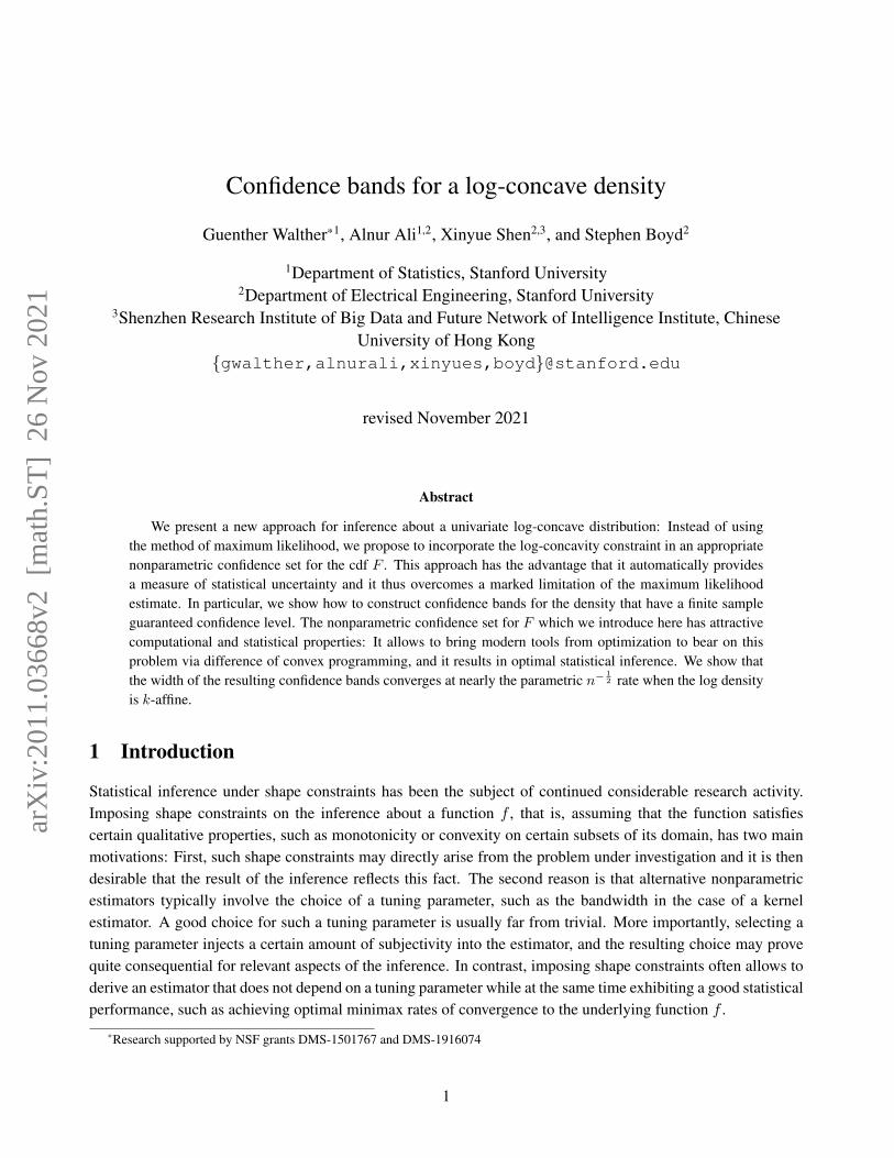
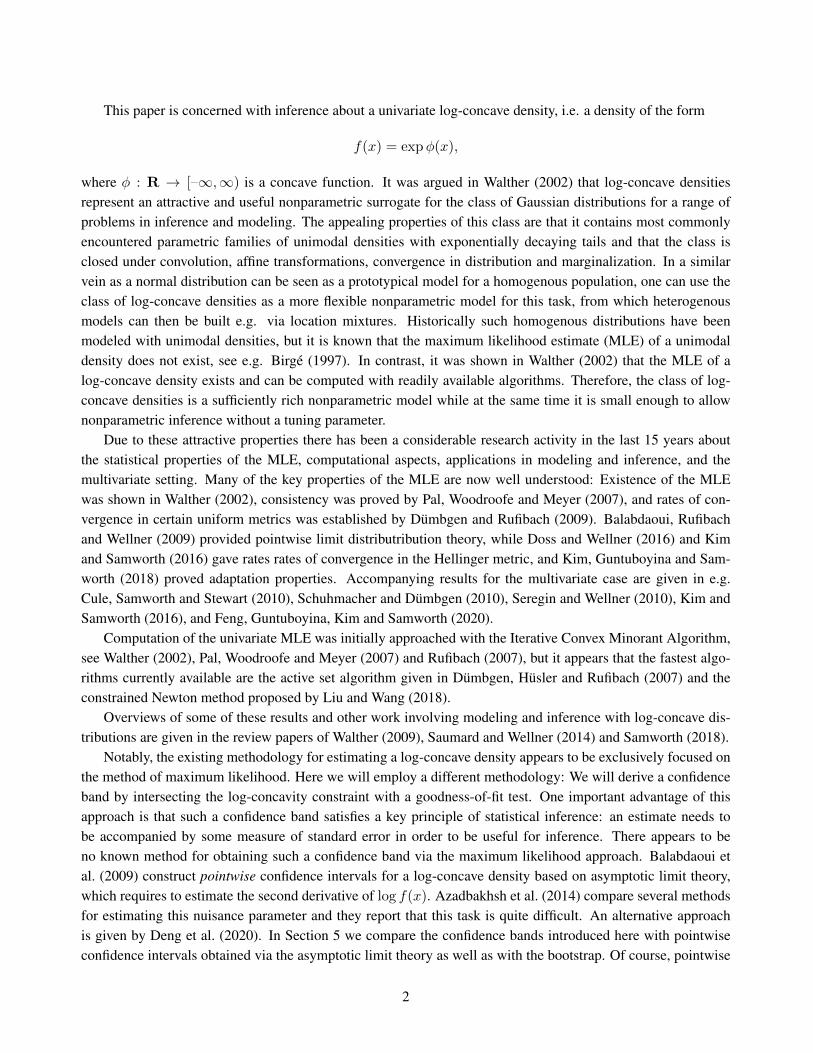
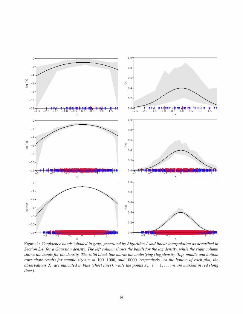
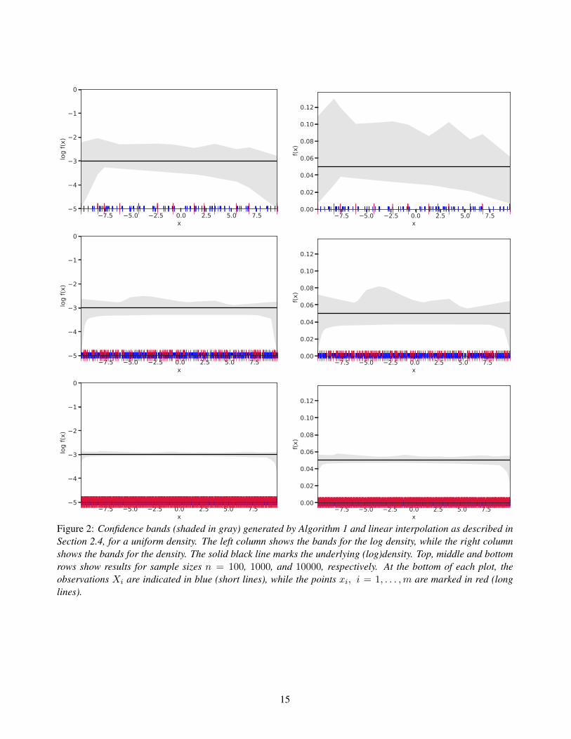
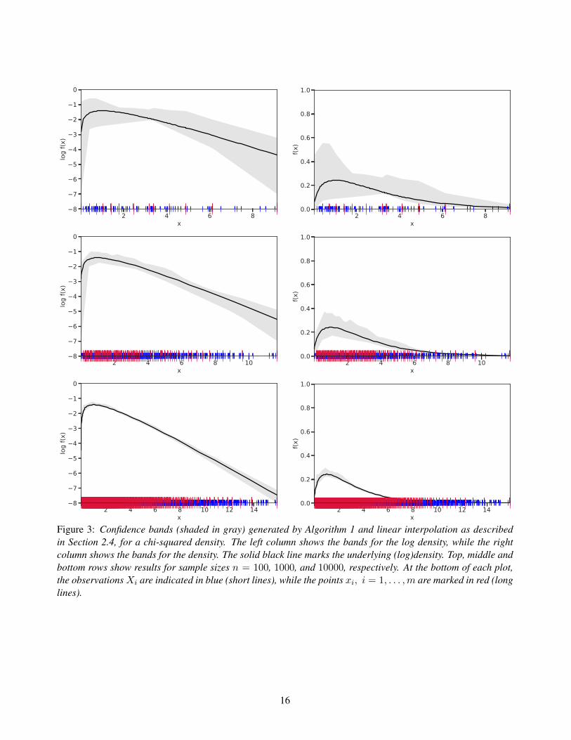
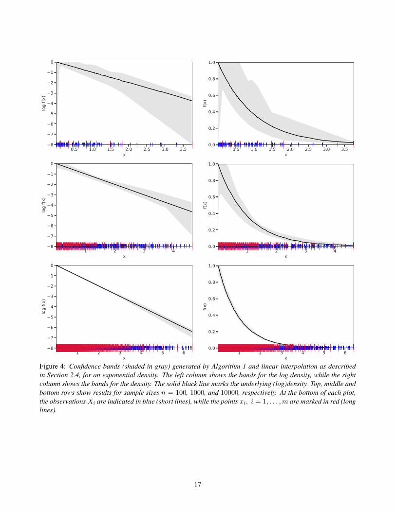
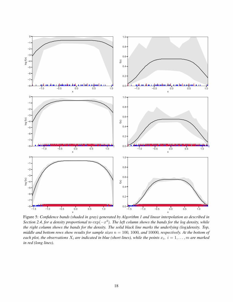
Table 1 summarizes the results. The table (reassuringly) shows us that the bands achieve coverage at orabove the nominal level. In Figures 1–5 we present a visualization of the bands, from a single repetition chosenat random, for each of the four underlying densities as well as for a density that is proportional to exp(−x4). Inaddition, we depict the bands for the case of a larger sample with n = 10000. The figures and Table 1 show thatwhile the bands are naturally wider when the sample size is small (n = 100), they quickly tighten as the samplesize grows (n ∈ {1000, 10000}).
As for the computational cost, we found that around 20-30 iterations of Algorithm 1 were enough to reachconvergence, for each point xi, i = 1, . . . ,m. Table 1 shows that this translates into just a few seconds tocompute the entire band when n = 100, and a couple of minutes when n = 1000. We found that Algorithm 1converged to the exact same solutions even when started from a number of different initial points, suggesting thatit is in fact finding the global minimizers of the problems (9). Therefore, these runtimes appear to be reasonable,as it is worth bearing in mind that Algorithm 1 is effectively solving a potentially large number of non-convexoptimization problems (precisely: 13, 39, and 188 such problems, corresponding to n ∈ {100, 1000, 10000},respectively). Moreover, we point out that the computation in Algorithm 1 can easily be parallelized, e.g. acrossthe points xi, i = 1, . . . ,m.
In order to compare the confidence band with pointwise confidence intervals, we performed these experi-ments also with two methods that compute pointwise confidence intervals for log-concave densities. Azadbakhshet al. (2014) compare several such methods and report that no one approach appears to uniformly dominate theothers and that each method works well only in a certain range of the data. The first group of methods examinedby Azadbakhsh et al. (2014) is based on the pointwise asymptotic theory developed in Balabdaoui et al. (2009)and requires estimating a nuisance parameter, for which Azadbakhsh et al. (2014) investigate several options. Wepicked the option that they report works best, namely their method (iv) in their Section 4. This method is called‘Asymptotic theory with approximation’ in Table 2. The second group of methods analyzed by Azadbakhsh etal. (2014) concerns various bootstrapping schemes, and we chose the one that they report to have the best perfor-mance, namely the ECDF-bootstrap, listed as (v) in their Section 4, which we use with 250 bootstrap repetitions.This method computes the MLE for each bootstrap sample and then computes the bootstrap percentile intervalat a point x0 based on the 250 bootstrap replicates of the MLE at x0. We used the R function logConCI pro-duced by Azadbakhsh et al. (2014) for implementing both methods. With each of the two methods we computethe pointwise 90% confidence interval for each point x0 in the grid of points that we use to evaluate empiricalcoverage. Since these are pointwise 90% confidence intervals, we expect that the coverage for the band (i.e. thesimultaneous coverage across all x0 in the grid) is smaller than 90%, but that the intervals are narrower thanthose for a simultaneous confidence band. This is confirmed by the results in Table 2, which show that both
12
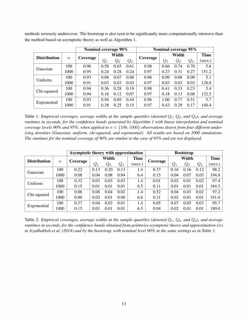
methods seriously undercover. The bootstrap is also seen to be significantly more computationally intensive thanthe method based on asymptotic theory as well as Algorithm 1.
Nominal coverage 90% Nominal coverage 95%
Distribution n Coverage Width Coverage Width TimeQ1 Q2 Q3 Q1 Q2 Q3 (secs.)
Gaussian100 0.96 0.58 0.65 0.61 0.98 0.66 0.74 0.70 5.61000 0.95 0.24 0.28 0.24 0.97 0.27 0.31 0.27 151.2
Uniform100 0.93 0.08 0.07 0.08 0.96 0.09 0.08 0.09 5.11000 0.91 0.03 0.03 0.03 0.97 0.03 0.03 0.03 128.8
Chi-squared100 0.94 0.36 0.28 0.19 0.98 0.41 0.33 0.23 5.41000 0.94 0.16 0.12 0.07 0.97 0.18 0.13 0.08 132.5
Exponential100 0.93 0.94 0.69 0.44 0.96 1.06 0.77 0.51 5.71000 0.91 0.38 0.25 0.15 0.97 0.43 0.29 0.17 140.4
Table 1: Empirical coverages, average widths at the sample quartiles (denoted Q1, Q2, and Q3), and averageruntimes in seconds, for the confidence bands generated by Algorithm 1 with linear interpolation and nominalcoverage levels 90% and 95%, when applied to n ∈ {100, 1000} observations drawn from four different under-lying densities (Gaussian, uniform, chi-squared, and exponential). All results are based on 1000 simulations.The runtimes for the nominal coverage of 90% are similar to the case of 95% and are not displayed.
Asymptotic theory with approximation Bootstrap
Distribution n Coverage Width Time Coverage Width TimeQ1 Q2 Q3 (secs.) Q1 Q2 Q3 (secs.)
Gaussian100 0.22 0.13 0.20 0.13 1.4 0.37 0.16 0.16 0.12 98.2
1000 0.08 0.04 0.08 0.04 6.4 0.15 0.04 0.07 0.03 194.8
Uniform100 0.32 0.03 0.03 0.03 1.4 0.01 0.02 0.01 0.02 97.4
1000 0.15 0.01 0.01 0.01 6.5 0.11 0.01 0.01 0.01 184.5
Chi-squared100 0.06 0.08 0.04 0.02 1.4 0.52 0.04 0.03 0.02 97.2
1000 0.00 0.02 0.01 0.00 6.6 0.31 0.02 0.01 0.01 191.0
Exponential100 0.37 0.04 0.02 0.01 1.4 0.05 0.07 0.05 0.03 95.7
1000 0.15 0.01 0.01 0.01 6.5 0.04 0.02 0.01 0.01 180.0
Table 2: Empirical coverages, average widths at the sample quartiles (denoted Q1, Q2, and Q3), and averageruntimes in seconds, for the confidence bands obtained from pointwise asymptotic theory and approximation (iv)in Azadbakhsh et al. (2014) and by the bootstrap, with nominal level 90% in the same settings as in Table 1.
13
−2.5 −2.0 −1.5 −1.0 −0.5 0.0 0.5 1.0 1.5x
−12
−10
−8
−6
−4
−2
0
log
f(x)
−2.5 −2.0 −1.5 −1.0 −0.5 0.0 0.5 1.0 1.5x
0.0
0.2
0.4
0.6
0.8
1.0
f(x)
−3 −2 −1 0 1 2x
−12
−10
−8
−6
−4
−2
0
log
f(x)
−3 −2 −1 0 1 2x
0.0
0.2
0.4
0.6
0.8
1.0f(x
)
−3 −2 −1 0 1 2x
−12
−10
−8
−6
−4
−2
0
log
f(x)
−3 −2 −1 0 1 2x
0.0
0.2
0.4
0.6
0.8
1.0
f(x)
Figure 1: Confidence bands (shaded in gray) generated by Algorithm 1 and linear interpolation as described inSection 2.4, for a Gaussian density. The left column shows the bands for the log density, while the right columnshows the bands for the density. The solid black line marks the underlying (log)density. Top, middle and bottomrows show results for sample sizes n = 100, 1000, and 10000, respectively. At the bottom of each plot, theobservations Xi are indicated in blue (short lines), while the points xi, i = 1, . . . ,m are marked in red (longlines).
14
−7.5 −5.0 −2.5 0.0 2.5 5.0 7.5x
−5
−4
−3
−2
−1
0
log
f(x)
−7.5 −5.0 −2.5 0.0 2.5 5.0 7.5x
0.00
0.02
0.04
0.06
0.08
0.10
0.12
f(x)
−7.5 −5.0 −2.5 0.0 2.5 5.0 7.5x
−5
−4
−3
−2
−1
0
log
f(x)
−7.5 −5.0 −2.5 0.0 2.5 5.0 7.5x
0.00
0.02
0.04
0.06
0.08
0.10
0.12
f(x)
−7.5 −5.0 −2.5 0.0 2.5 5.0 7.5x
−5
−4
−3
−2
−1
0
log
f(x)
−7.5 −5.0 −2.5 0.0 2.5 5.0 7.5x
0.00
0.02
0.04
0.06
0.08
0.10
0.12
f(x)
Figure 2: Confidence bands (shaded in gray) generated by Algorithm 1 and linear interpolation as described inSection 2.4, for a uniform density. The left column shows the bands for the log density, while the right columnshows the bands for the density. The solid black line marks the underlying (log)density. Top, middle and bottomrows show results for sample sizes n = 100, 1000, and 10000, respectively. At the bottom of each plot, theobservations Xi are indicated in blue (short lines), while the points xi, i = 1, . . . ,m are marked in red (longlines).
15
2 4 6 8x
−8
−7
−6
−5
−4
−3
−2
−1
0
log
f(x)
2 4 6 8x
0.0
0.2
0.4
0.6
0.8
1.0
f(x)
2 4 6 8 10x
−8
−7
−6
−5
−4
−3
−2
−1
0
log
f(x)
2 4 6 8 10x
0.0
0.2
0.4
0.6
0.8
1.0
f(x)
2 4 6 8 10 12 14x
−8
−7
−6
−5
−4
−3
−2
−1
0
log
f(x)
2 4 6 8 10 12 14x
0.0
0.2
0.4
0.6
0.8
1.0
f(x)
Figure 3: Confidence bands (shaded in gray) generated by Algorithm 1 and linear interpolation as describedin Section 2.4, for a chi-squared density. The left column shows the bands for the log density, while the rightcolumn shows the bands for the density. The solid black line marks the underlying (log)density. Top, middle andbottom rows show results for sample sizes n = 100, 1000, and 10000, respectively. At the bottom of each plot,the observationsXi are indicated in blue (short lines), while the points xi, i = 1, . . . ,m are marked in red (longlines).
16
0.5 1.0 1.5 2.0 2.5 3.0 3.5x
−8
−7
−6
−5
−4
−3
−2
−1
0
log
f(x)
0.5 1.0 1.5 2.0 2.5 3.0 3.5x
0.0
0.2
0.4
0.6
0.8
1.0
f(x)
1 2 3 4x
−8
−7
−6
−5
−4
−3
−2
−1
0
log
f(x)
1 2 3 4x
0.0
0.2
0.4
0.6
0.8
1.0
f(x)
1 2 3 4 5 6x
−8
−7
−6
−5
−4
−3
−2
−1
0
log
f(x)
1 2 3 4 5 6x
0.0
0.2
0.4
0.6
0.8
1.0
f(x)
Figure 4: Confidence bands (shaded in gray) generated by Algorithm 1 and linear interpolation as describedin Section 2.4, for an exponential density. The left column shows the bands for the log density, while the rightcolumn shows the bands for the density. The solid black line marks the underlying (log)density. Top, middle andbottom rows show results for sample sizes n = 100, 1000, and 10000, respectively. At the bottom of each plot,the observationsXi are indicated in blue (short lines), while the points xi, i = 1, . . . ,m are marked in red (longlines).
17
−1.0 −0.5 0.0 0.5 1.0x
−8
−7
−6
−5
−4
−3
−2
−1
0
log
f(x)
−1.0 −0.5 0.0 0.5 1.0x
0.0
0.2
0.4
0.6
0.8
1.0
f(x)
−1.0 −0.5 0.0 0.5 1.0x
−8
−7
−6
−5
−4
−3
−2
−1
0
log
f(x)
−1.0 −0.5 0.0 0.5 1.0x
0.0
0.2
0.4
0.6
0.8
1.0
f(x)
−1.5 −1.0 −0.5 0.0 0.5 1.0x
−8
−7
−6
−5
−4
−3
−2
−1
0
log
f(x)
−1.5 −1.0 −0.5 0.0 0.5 1.0x
0.0
0.2
0.4
0.6
0.8
1.0
f(x)
Figure 5: Confidence bands (shaded in gray) generated by Algorithm 1 and linear interpolation as described inSection 2.4, for a density proportional to exp(−x4). The left column shows the bands for the log density, whilethe right column shows the bands for the density. The solid black line marks the underlying (log)density. Top,middle and bottom rows show results for sample sizes n = 100, 1000, and 10000, respectively. At the bottom ofeach plot, the observations Xi are indicated in blue (short lines), while the points xi, i = 1, . . . ,m are markedin red (long lines).
18

6 Proofs
Proof of Lemma 1: It is well known that if log f(x) is a concave function then there exist real numbersg1, . . . , gm such that
log f(x) ≤ `i + gi (x− xi) for i = 1, . . . ,m,
see e.g. Boyd and Vandenberghe (2004). We found it computationally advantageous to employ these inequalitiesonly for i = 2, . . . ,m− 1. Those inequalities immediately yield
`j ≤ `i + gi (xj − xi) for all i ∈ {2, . . . ,m− 1}, j ∈ {i− 1, i+ 1}, (15)
as well as for i = 2, . . . ,m− 1:∫ xi+1
xi
f(x) dx ≤ exp(`i)
∫ xi+1
xi
exp(gi(x− xi)
)dx = exp(`i)(xi+1 − xi)E
(gi(xi+1 − xi)
)and for i = 1, . . . ,m− 2:∫ xi+1
xi
f(x) dx ≤ exp(`i+1)
∫ xi+1
xi
exp(gi+1(x− xi+1)
)dx = exp(`i+1)(xi+1 − xi)E
(gi+1(xi − xi+1)
).
On the other hand, since log f is concave on (xi, xi+1) it cannot be smaller than the chord from xi to xi+1.Hence for i = 1, . . . ,m− 1:∫ xi+1
xi
f(x) dx ≥∫ xi+1
xi
exp(`i + (x− xi)
`i+1 − `ixi+1 − xi
)dx = (xi+1 − xi) exp(`i)E
(`i+1 − `i
),
proving the lemma. For later use we note the following fact:
If (15) holds, then (15) holds for all j ∈ {1, . . . ,m}, and the gi are non-increasing in i. (16)
This is because (15) implies both `i+1 ≤ `i + gi(xi+1 − xi) and `i ≤ `i+1 + gi+1(xi − xi+1), hence gi ≥`i+1−`ixi+1−xi ≥ gi+1. This monotonicity property and (15) yield for j > i:
`j ≤j−1∑k=i
gk(xk+1 − xk) + `i ≤ gij−1∑k=i
(xk+1 − xk) + `i = `i + gi(xj − xi)
and analogously for j < i. 2
Proof of Theorem 1: Let d > 0 be an integer that will be determined later as a function of f, I, J , and setB := Bmax − d. So d does not change with n but B does as Bmax increases with n. Define the event
An(d) :=
{∣∣∣∣∣∫ xk
xj
f(t) dt− pjk
∣∣∣∣∣ ≤√pjk(1− pjk)
n
√log logn for all (j, k) ∈ IB
}
where pjk := k−jn+12sn . We will prove the theorem with a sequence of lemmata. The first lemma bounds the width
of the confidence band on the discrete set {xj , j ∈ K}, where K := {j : j = 1 + i2B with 3 ≤ i ≤ nB − 3 and(xj−3·2B , xj+3·2B ) ⊂ J}:
19

Lemma 2 If {`1, . . . , `m g2, . . . , gm−1} is a feasible point for the optimization problem (9), then on An(d)
maxj∈K|`j − log f(xj)| ≤ 17
√2d
log log n
n.
In order to extend the bound over the discrete set {xj , j ∈ K} to a uniform bound over the interval I we willuse the following fact, which is readily proved using elementary calculations:
If the linear function L(t) and the concave function g(t) satisfy |L(ti) − g(ti)| ≤ D for t1 < t2 < t3 < t4,then supt∈(t2,t3) |L(t)− g(t)| ≤ D
(1 + 2 min
(t3−t2t2−t1 ,
t3−t2t4−t3
)).
Lemma 3 On the event An(d)
min
(maxj∈K
xj+2B − xjxj − xj−2B
,maxj∈K
xj+2B − xjxj+2·2B − xj+2B
)≤ 9
8.
Therefore any concave function g for which {g(xj), j ∈ K} is feasible for (9) must satisfy
supx∈[x
j+2B,x
j−2B]
∣∣∣g(x)− log f(x)∣∣∣ ≤ 13
417
√2d
log log n
n
on An(d), where j := minK and j := maxK. Hence this bound applies to the lower and upper confidencelimits ˆ and µ since ˆ is a concave function and {ˆ(xi), i = 1, . . . ,m} is feasible for (9), and for every real xthere exist a concave function g such that g(x) = µ(x) and {g(xi), i = 1, . . . ,m} is feasible for (9).
In order to conclude the proof of the theorem we will show
Lemma 4IP {An(d)} → 1 as n→∞
and
Lemma 5IP{I ⊂ (xj−2B , xj+2B )
}→ 1 as n→∞
for a certain d = d(f, I, J).
Then the claim of the theorem follows since the bound on the log densities carries over to the densities assupx∈I |g(x)− log f(x)| ≤ 1 implies
supx∈I
∣∣∣exp(g(x))− f(x)∣∣∣ ≤ 2
(supx∈I
f(x))
supx∈I
∣∣∣g(x)− log f(x)∣∣∣.
It remains to prove the Lemmata 2–5. We will use the following two facts:
Fact 1 If L(x) is a linear function, then∫ βα exp(L(x)) dx = (β − α) exp(L(α))E
(L(β)− L(α)
), where E(·)
is given in Lemma 1. One readily checks that the function R2 3 (s, t) 7→ exp(t)E(s− t) is increasing in both s
20

and t. Furthermore, since sinh(x)x is increasing for x > 0 we have for s < t and C > 0:
exp(t+ C)E(s− (t+ C)
)=
exp(s)− exp(t+ C)
s− (t+ C)
= exp
(s+ t+ C
2
)sinh
(t+C−s
2
)t+C−s
2
≥ exp
(C
2
)exp
(s+ t
2
)sinh
(t−s2
)t−s2
≥(
1 +C
2
)exp(s)− exp(t)
s− t
=
(1 +
C
2
)exp(t)E(s− t)
and this inequality also holds for s = t since E is continuous.
Fact 2 Let k ∈ (0, n+ 1) and p := kn+1 . Then for α ∈ (0, 1)
qBeta (1− α, k, n+ 1− k)− p
−(qBeta (α, k, n+ 1− k)− p
) ≤√p(1− p)n+ 1
√2 log
1
α+
log 1α
n+ 1
where qBeta (α, r, s) denotes the α-quantile of the beta distribution with parameters r and s. This fact followsfrom Propostion 2.1 in Dumbgen (1998).
Proof of Lemma 2: Since log f is linear on J we will assume that it is non-increasing on J . The non-decreasingcase is proved analogously. Let j ∈ K and set k := j + 2B , so (j, k) ∈ IB . The concavity constraint (5) impliesthat the function hjk(t) :=
∑k−1i=j 1(xi ≤ t < xi+1)
(`i + (t− xi) `i+1−`i
xi+1−xi
)is concave on (xj , xk) and hence
not smaller than its secant gjk(t) := `j + (t− xj) `k−`jxk−xj . Hence
k−1∑i=j
(xi+1 − xi) exp(`i)E(`i+1 − `i) =k−1∑i=j
∫ xi+1
xi
exp
(`i + (t− xi)
`i+1 − `ixi+1 − xi
)dt
=
∫ xk
xj
exp (hjk(t)) dt
≥∫ xk
xj
exp (gjk(t)) dt
= (xk − xj) exp(`j)E(`k − `j) (17)
Suppose `j > log f(xj) + C where C := 17 · 2d2
√log logn
n . If `k ≥ log f(xk) then Fact 1 shows (note that
21
log f(xj) ≥ log f(xk) as f is non-increasing) that (17) is not smaller than
(xk − xj) exp(log f(xj) + C
)E(
log f(xk)− (log f(xj) + C))
≥ (xk − xj)(
1 +C
2
)exp (log f(xj)) E
(log f(xk)− log f(xj)
)=
(1 +
C
2
)∫ xk
xj
f(t) dt (18)
since log f(t) is linear on (xj , xk). Now pjk ≥ 2−d−4 since B = Bmax − d, and hence C ≥ 174
√log lognpjkn
. So
on the event An(d), (18) is not smaller than(1 +
17
8
√log log n
pjk n
)(pjk −
√pjk(1− pjk)
n
√log log n
)
> pjk +9
8
√pjk(1− pjk)
n
√log logn
> qBeta(
1− α
2(B + 2)nBtn, (k − j)2sn , n+ 1− (k − j)2sn
)= dB
by Fact 2, since B = Bmax − d implies nB ≤ n2Bmax+sn−d ≤ 16 · 2d, while tn ≤ log(Bmax + 2) ≤ log log2 n,
and therefore 2(B + 2)nBtn ≤ α(log n)2 for n large enough. Thus we arrive at a violation of the constraint (8).On the other hand, suppose `j > log f(xj) + C and `k < log f(xk). Set k = j + 2B , r := j + 2 · 2B and
s := j + 3 · 2B . Then xr − xk ≥ 89(xk − xj) by (21). By (5) and (16)
gi ≤ gk ≤`k − `jxk − xj
≤ log f(xk)− log f(xj)− Cxk − xj
for i = k, . . . , s− 1.
Hence for k ≤ i < m ≤ s− 1:
gi(xm − xi) ≤ log f(xm)− log f(xi)−xm − xixk − xj
C (19)
since log f is linear on (xk, xs). This yields
`r ≤ `k + gk(xr − xk)
≤ log f(xk) + log f(xr)− log f(xk)−xr − xkxk − xj
C
≤ log f(xr)−8
9C
and likewise for m = r + 1, . . . , s− 1:
`m ≤ `r + gr(xm − xr)
≤ log f(xr)−8
9C + log f(xm)− log f(xr)−
xm − xrxk − xj
C
≤ log f(xm)− 8
9C
22
Since the function E(s) is positive and increasing for s ∈ R we obtain with (19):
s−1∑i=r
exp(`i)(xi+1 − xi)E (gi(xi+1 − xi))
≤s−1∑i=r
exp
(log f(xi)−
8
9C
)(xi+1 − xi)E
(log f(xi+1)− log f(xi)
)= exp
(−8
9C
) s−1∑i=r
∫ xi+1
xi
exp(
log f(t))dt
<
(1− 7
9C
)∫ xs
xr
f(t) dt since C ∈[174
√log lognprsn
, 14
]≤
(1− 7 · 17
9 · 4
√log log n
prsn
)(prs +
√prs(1− prs)
n
√log logn
)on An(d)
< prs − 2
√prs(1− prs)
n
√log logn
< qBeta(
α
2(B + 2)nBtn, (s− r)2sn , n+ 1− (s− r)2sn
)= cB
by Fact 2, yielding a violation of (7). Therefore we conclude `j ≤ log f(xj) + C as claimed. The lower boundfor `j follows analogously. 2
Proof of Lemma 3: f is monotone on J since it is log-linear. Consider first the case where f is non-increasingon J . On An(d) we have for j ∈ K and k := j + 2B , r := j + 2 · 2B:
∫ xrxkf(t) dt∫ xk
xjf(t) dt
≥pkr −
√pkr(1−pkr)
n
√log logn
pjk +
√pjk(1−pjk)
n
√log log n
≥ 8
9(20)
for n large enough, since pkr = pjk ≥ 2−d−4. Since f is non-increasing on J , (20) implies
xk − xj ≤∫ xk
xj
f(t)
f(xk)dt ≤ 9
8
∫ xr
xk
f(t)
f(xk)dt ≤ 9
8(xr − xk) (21)
and the claim of the Lemma follows. If f is non-decreasing on J then we obtain analogously xj+2B − xj ≤98(xj − xj−2B ) for all j ∈ K and the claim of the Lemma follows also. 2
Proof of Lemma 4: Set αn := (log n)−13 . Then for (j, k) ∈ IB√
pjk(1− pjk)n+ 1
√2 log
1
αn+
log 1αn
n+ 1≤√pjk(1− pjk)
n
√log logn
for n large enough as pjk = k−jn+12sn = 2B+sn
n+1 ∼2−d
8 . There are nB ≤ n2Bmax+sn−d ≤ 16 · 2d tuples (j, k) in IB
and ∫ xk
xj
f(t) dt ∼ Beta (2B+sn , n+ 1− 2B+sn).
23
Hence, setting j := 1, k := 1 + 2B and using Fact 2:
IP{An(d)c
}≤ nB IP
{∣∣∣∣∣∫ xk
xj
f(t) dt− pjk
∣∣∣∣∣ >√pjk(1− pjk)
n
√log logn
}
≤ 16 · 2d IP
{∫ xk
xj
f(t) dt 6∈(qBeta (αn, 2
B+sn , n+ 1− 2B+sn), qBeta (1− αn, 2B+sn , n+ 1− 2B+sn))}
= 16 · 2d(2αn) → 0
2
Proof of Lemma 5: Note that J \ I = D1 ∪D2, where D1 is the interval between the left endpoints of I andJ , and D2 is the interval between the right endpoints. Recall that j is the smallest index j = 1 + i2B such thatxj−3·2B ∈ J . Hence xj−3·2B and xj−2B must both fall into D1 if at least 4 · 2B points xi fall into D1, i.e. if atleast 4 · 2B+sn observations Xi fall into D1. Therefore
IP{I ⊂
(xj−2B , xj+2B
)}≥ IP
{Fn(Di) ≥
4 · 2B+sn
n, i = 1, 2
}where Fn denotes the empirical distribution. Since f is log-linear on J :
q := q(f, I, J) := min
(∫D1
f(t) dt,
∫D2
f(t) dt
)> 0.
Therefore
42B+sn
n− F (D1) ≤ 4
2log2n8−d
n− q = 2−1−d − q < 0
for d > log212q , in which case Chebychev’s inequality gives
IP
{Fn(D1) < 4
2B+sn
n
}≤ 1
4n(2−1−d − q)2→ 0
and the same result holds for Fn(D2). 2
References
Azadbakhsh, M., Jankowski, H. and Gao, X. (2014). Computing confidence intervals for log-concave densities.Comput. Statist. Data Anal. 75, 248–264.
Balabdaoui, F., Rufibach, K. and Wellner, J. A. (2009). Limit distribution theory for maximum likelihoodestimation of a log-concave density. Ann. Statist. 37, 1299–1331.
Birge, L. (1997). Estimation of unimodal densities without smoothness assumptions. Ann. Statist. 25, 970–981.
Boyd, S. and Vandenberghe, L. (2004). Convex Optimization. Cambridge University Press, New York.
Chan, H.P. and Walther, G. (2013). Detection with the scan and the average likelihood ratio. Statist. Sinica 23,409–428.
24
Cule, M., Samworth, R. and Stewart, M. (2010). Maximum likelihood estimation of a multi-dimensional log-concave density. J. R. Stat. Soc. Ser. B Stat. Methodol. 72, 545–607.
Davies, P.L. and Kovac, A. (2004). Densities, spectral densities and modality. Ann. Statist. 32, 1093-1136.
Deng, H., Han, Q. and Sen, B. (2020). Inference for local parameters in convexity constrained models. arXivpreprint arXiv:2006.10264.
Dinh, T. P. and Le Thi, H. A. (2014). Recent advances in DC programming and DCA. In Transactions oncomputational intelligence XIII, 1-37. Springer, Berlin, Heidelberg.
Donoho, D.L. (1988). One-sided inference for functionals of a density. Ann. Statist. 16, 1390-1420.
Doss, C. R. and Wellner, J. A. (2016). Global rates of convergence of the MLEs of log-concave and s-concavedensities. Ann. Statist. 44, 954–981.
Dumbgen, L. (1998). New goodness-of-fit tests and their application to nonparametric confidence sets. Ann.Statist. 26, 288–314.
Dumbgen, L. (2003). Optimal confidence bands for shape-restricted curves. Bernoulli 9, 423–449.
Dumbgen, L., Husler, A. and Rufibach, K. (2007). Active set and EM algorithms for log-concave densitiesbased on complete and censored data. arXiv preprint arXiv:0707.4643v4.
Dumbgen, L. and Rufibach, K. (2009). Maximum likelihood estimation of a log-concave density and its distri-bution function: basic properties and uniform consistency. Bernoulli 15, 40–68.
Feng, O., Guntuboyina, A., Kim, A. K. H. and Samworth, R. J. (2020+). Adaptation in multivariate log-concavedensity estimation. Ann. Statist., to appear.
Hartman, P. (1959). On functions representable as a difference of convex functions. Pacific Journal of Mathe-matics 9(3), 707-713.
Hengartner, N.W. and Stark, P.B. (1995). Finite-sample confidence envelopes for shaperestricted densities.Ann. Statist. 23, 525–550.
Horst, R., Pardalos, P. M. and Van Thoai, N. (2000). Introduction to global optimization. Springer Science andBusiness Media.
Horst, R. and Thoai, N. V. (1999). DC programming: overview. Journal of Optimization Theory and Applica-tions 103(1), 1-43.
Khamaru, K. and Wainwright, M. J. (2018). Convergence guarantees for a class of non-convex and non-smoothoptimization problems. arXiv preprint arXiv:1804.09629.
Kim, A. K. H. and Samworth, R. J. (2016). Global rates of convergence in log-concave density estimation.Ann. Statist. 44, 2756–2779.
Kim, A. K. H., Guntuboyina, A. and Samworth, R. J. (2018). Adaptation in log-concave density estimation.Ann. Statist. 46, 2279–2306.
25
Le Thi, H. A. and Dinh, T. P. (2014). DC programming and DCA for general DC programs. In AdvancedComputational Methods for Knowledge Engineering, 15-35. Springer, Cham.
Li, H., Munk, A., Sieling, H. and Walther, G. (2020). The essential histogram. Biometrika 107, 347–364.
Lipp, T. and Boyd, S. (2016). Variations and extension of the convex–concave procedure. Optimization andEngineering 17(2), 263-287.
Liu, Y. and Wang, Y. (2018). A fast algorithm for univariate log-concave densityi estimation. Aust. N. Z. J.Stat. 60(2), 258–275.
Pal, J. K., Woodroofe, M. and Meyer, M. (2007). Estimating a Polya frequency function. In Complex datasetsand inverse problems. IMS Lecture Notes Monogr. Ser. 54, 239–249. Inst. Math. Statist., Beachwood,OH.
Rivera, C. and Walther, G. (2013). Optimal detection of a jump in the intensity of a Poisson process or in adensity with likelihood ratio statistics. Scand. J. Stat. 40, 752–769.
Samworth, R.J. (2018). Recent progress in log-concave density estimation. Statist. Sci. 33, 493-509.
Saumard, A. and Wellner, J.A. (2014). Log-concavity and strong log-concavity: a review. Statistics Surveys 8,45-114.
Schuhmacher, D. and Dumbgen, L. (2010). Consistency of multivariate log-concave density estimators. Statist.Probab. Lett. 80, 376–380.
Seregin, A. and Wellner, J. A. (2010). Nonparametric estimation of multivariate convex-transformed densities.Ann. Statist. 38, 3751–3781.
Shorack, G.R. and Wellner, J.A. (1986). Empirical Processes with Applications to Statistics. Wiley, New York.
Smola, A. J., Vishwanathan, S. V. N. and Hofmann, T. (2005). Kernel Methods for Missing Variables. InAISTATS.
Sriperumbudur, B. K. and Lanckriet, G. R. (2009, December). On the convergence of the concave-convex pro-cedure. In Proceedings of the 22nd International Conference on Neural Information Processing Systems,1759-1767. Curran Associates Inc.
Tao, P. D. (1986). Algorithms for solving a class of nonconvex optimization problems. Methods of subgradients.In North-Holland Mathematics Studies 129, 249-271. North-Holland.
Walther, G. (2002). Detecting the presence of mixing with multiscale maximum likelihood. J. Amer. Statist.Assoc. 97, 508–513.
Walther, G. (2009). Inference and modeling with log-concave distributions. sl Statist. Sci. 24, 319–327.
Walther, G. (2010). Optimal and fast detection of spatial clusters with scan statistics. Ann. Statist. 38,1010–1033.
Walther, G. and Perry, A. (2019). Calibrating the scan statistic: finite sample performance vs. asymptotics.arXiv preprint arXiv:2008.06136.
26

Yuille, A. L. and Rangarajan, A. (2003). The concave-convex procedure. Neural computation 15(4), 915-936.
27
Recommended