DELPH Seismic
Interpretation
User Guide

DELPH Seismic Interpretation – User Guide
Copyright All rights reserved. No part of this guide may be reproduced or transmitted, in any form or
by any means, whether electronic, printed guide or otherwise, including but not limited to
photocopying, recording or information storage and retrieval systems, for any purpose
without prior written permission of iXBlue.
Disclaimer iXBlue specifically disclaims all warranties, either express or implied, included but not
limited to implied warranties of merchantability and fitness for a particular purpose with
respect to this product and documentation. iXBlue reserves the right to revise or make
changes or improvements to this product or documentation at any time without notify any
person of such revision or improvements.
In no event shall iXBlue be liable for any consequential or incidental damages, including
but not limited to loss of business profits or any commercial damages, arising out of the
use of this product.
MU-DSI-AN-v30 Ed. A – May 2014 i
DELPH Seismic Interpretation – User Guide
Warranty
iXBlue warrants that the Software will perform substantially in accordance with the
accompanying written materials for a period of twelve (12) months from the date of
shipment.
iXBlue’s entire liability and your exclusive remedy shall be, at iXBlue’s option, repair or
replacement of the Software that does not meet iXBlue’s Limited Warranty. Warranty
service is F.O.B. iXBlue France. All shipping and insurance costs to iXBlue are paid by
buyer; shipping and insurance costs returning to buyer will be paid by iXBlue.
On-site Customer Service and Warranty Repair may be provided by iXBlue, at its own
discretion. Travel and accommodations (including travel hours, transportation, lodging and
meals) will be charged by iXBlue to Buyer at cost plus ten (10) percent. However, actual
labor hours to provide this service or repair will be free of charge to Buyer. This Limited
Warranty is void if failure of the Software or hardware has resulted from accident, abuse,
or misapplication. Any replacement Software or hardware will be warranted for the
remainder of the original warranty period or thirty (30) days, whichever is longer.
iXBlue makes no other warranties than the above limited warranties. iXBlue makes no
warranties, expressed, implied, statutory, or in any communication with you, and iXBlue
specifically disclaims any implied warranty of merchantability or fitness for a particular
purpose. iXBlue does not warrant that the operation of the program will be uninterrupted
or error free.
To the maximum extent permitted by applicable law, in no event shall iXBlue be liable for
any damages whatsoever (including, without limitation, damages for loss of business
profits, business interruption, loss of business information, or any other pecuniary loss)
arising out of the use of or inability to use this iXBlue product, even if iXBlue has been
advised of the possibility of such damages.
iXBlue will not replace lost dongles free, neither offer discounted pricing terms for
replacement dongles.
iXBlue strongly recommends that you insure your iXBlue products against loss, theft or
damage where applicable.
iXBlue will propose the replacement of damaged dongles only for a limited fee, provided
that the damaged dongle units will be returned to iXBlue. All shipping and insurance costs
are paid by buyer.
1. Warranty period
2. Customer Remedies
3. Limitations
4. Liability
5. Dongles
MU-DSI-AN-v30 Ed. A – May 2014 ii
DELPH Seismic Interpretation – User Guide
Software License Agreement PLEASE READ THIS SOFTWARE LICENSE AGREEMENT CAREFULLY BEFORE
INSTALLING OR USING THE SOFTWARE.
BY CLICKING ON THE "ACCEPT" BUTTON, INSTALLING THE SOFTWARE, OR USING
THE SOFTWARE, YOU ARE CONSENTING TO BE BOUND BY THIS AGREEMENT. IF
YOU DO NOT AGREE TO ALL OF THE TERMS OF THIS AGREEMENT, CLICK THE
"DO NOT ACCEPT" BUTTON AND THE INSTALLATION PROCESS WILL NOT
CONTINUE, RETURN THE PRODUCT TO THE PLACE OF PURCHASE FOR A FULL
REFUND.
iXBlue grants you a nonexclusive and nontransferable license to use the enclosed iXBlue
software in the manner provided below:
• the number of software users depends on the licenses agreed by iXBlue. The user is
able to connect with a security key provided by iXBlue for use on a single computer;
• you may couple multiple iXBlue licenses on a single computer;
• you may make up to two (2) copies of the software for archival or backup purposes,
provided that you reproduce proprietary notices.
• You shall not share by any means, other than by agreement with iXBlue, the software
licenses between multiple computers.
• You shall not copy the software except as set forth in the section above. Any copy of
the software that you make must contain the same copyright and other proprietary
notices that appear on or in the software.
• You shall not modify, adapt or translate the software. You shall not reverse engineer,
decompile, disassemble or otherwise attempt to modify or discover the source code of
the software.
• You shall not install, neither operate the software on virtual machines.
• You shall not, rent, lease, sublicense, assign or transfer your rights in the software
without prior written authorization from iXBlue.
The software (including any images, animations and text incorporated into the software) is
owned by iXBlue and protected by copyright laws and international treaty provisions.
iXBlue offers software maintenance during the warranty period. This maintenance
includes the delivery of minor documentary and software licenses. The major or
intermediary updates are not included and shall be dealt with in a separate agreement. If
the software supplied under license is an updated version, the licensee will only be
allowed to use the software in order to replace versions of the same software previously
and duly acquired under license.
Extended Maintenance Agreements – E.M.A. – may be purchased to extend the product
maintenance after the warranty period. An E.M.A. shall be applied to every software
license that will be maintained and upgraded.
1. Grant of license
2. Restrictions
3. Copyright
4. Maintenance / Data update
5. Extended Maintenance
MU-DSI-AN-v30 Ed. A – May 2014 iii
DELPH Seismic Interpretation – User Guide
Technical support is available free of charge during the warranty period:
• On iXBlue website: http://www.ixblue.com/content/ixblue-support
• By dedicated e-mail box: [email protected]
• 24/7 hot-lines: +1 888 600 7573 Extension 2 (North America); +33 1 30 08 98 98
(Europe Middle-East Africa Latin-America); +65 6747 7027 (Asia Pacific)
The price comprises the main product together with accessories: grant of license and
accrued expenses (as referred to in the order, contract, or in the manufacturer or supplier
price list).
The user license is considered to be granted when iXBlue acknowledges reception of the
whole price paid by the Buyer. Payment is made by means of a secure electronic payment
system or by any other means authorized by iXBlue.
iXBlue will notify reception of payment by electronic mail.
In case of non-payment and/or non-respect of the present terms, all rights of the license
and the use of software will be terminated, without prejudice to any legal action iXBlue
may carry out against the defaulting party.
The Buyer will be obliged, at its own expense and risk, to return to iXBlue all copies of the
software under license in its possession together with physical protection keys, or to
confirm in writing that all software copies under license in its possession have been
destroyed.
iXBlue reserves the right to proceed to all the necessary verifications in order to be
assured of the buyer’s observance of the aforementioned conditions.
Both parties will do their utmost to bring an end to disputes relative to the interpretation
and/or the execution of this document by settling an agreement between their respective
management. If an agreement has not been reached within three months, the dispute will
be decided by the Paris tribunal jurisdiction.
6. Technical support
7. Price
8. Termination
9. Out-of-court settlement,
choice of jurisdiction
MU-DSI-AN-v30 Ed. A – May 2014 iv
DELPH Seismic Interpretation – User Guide
Overview of DELPH Seismic Interpretation User Guide
This document is the User Manual for DELPH Seismic Interpretation. It must be read and
understood prior to using the DELPH Seismic Interpretation software.
The manufacturer shall in no case be held liable for any application or use that does not
comply with the stipulations in this manual.
DELPH Seismic Interpretation User Manual is divided into several parts:
• Part 1: Introduction – This part introduces the software, its purpose, architecture and
functionalities.
• Part 2: Getting Started with DELPH Seismic Interpretation – This part helps the
beginner to go through the preliminary steps taking place before actual use of the
software.
• Part 3: Managing a Project – This part describes the project structure, the project
database selection, the geometry file and the geodesic settings.
• Part 4: DELPH RoadMap – This part is devoted to the 3D visualization application
common to all imagery data.
• Part 5: DELPH Seismic Interpretation – This part describes the functionalities
available in the software.
• Part 6: GeoSections – This part describes the GeoSection tool allowing advanced
geographic interpretation of the seismic profiles.
• Part 7: Digital Terrain Modeling – This part explains how to build DTMs from the
layers of seismic profiles.
The abbreviations and acronyms used in this manual are listed hereafter.
A Table of Contents is available in the following pages to allow a quick access to
dedicated information.
MU-DSI-AN-v30 Ed. A – May 2014 v
DELPH Seismic Interpretation – User Guide
Text Usage and Icons
bold Bold text is used for items you must select or click in the
software. It is also used for the field names used into the dialog
box. Courier Text in this font denotes text or characters that you should enter
from the keyboard, the proper names of disk Drives, paths,
directories, programs, functions, filenames and extensions.
italic Italic text is the result of an action in the procedures.
The Note icon indicates that the following information is of interest to the operator and
should be read.
MU-DSI-AN-v30 Ed. A – May 2014 vi
DELPH Seismic Interpretation – User Guide
Abbreviations and Acronyms
DTM Digital Terrain Model
GIS Geographic Information System
KP Kilometer Point
SEG-Y Society of Exploration Geophysicists seismic data format
SHP ESRI Shape File Format
TVF Time Varying Filter
XTF EXtended Triton Format.
MU-DSI-AN-v30 Ed. A – May 2014 vii
DELPH Seismic Interpretation – User Guide
Table of Contents
I INTRODUCTION ...........................................................................................................................1
II GETTING STARTED WITH DELPH SEISMIC INTERPRETATION ...........................................................4 II.1 System Requirements .........................................................................................................4
II.2 Managed and Created Files Types .....................................................................................4 II.3 Installing DELPH Seismic Interpretation ............................................................................5
II.4 Service Pack ........................................................................................................................7
II.5 Managing License ...............................................................................................................8 II.5.1 File Protection ..................................................................................................................8
II.5.2 Dongle Protection .............................................................................................................9
III MANAGING A PROJECT ..............................................................................................................11
III.1 Introduction .......................................................................................................................11 III.2 Project File Structure ........................................................................................................11
III.3 Creating or Selecting a Project Database ........................................................................12
III.4 Using an Geometry File from DELPH Acquisition ...........................................................14 IV DELPH ROADMAP ...................................................................................................................15
V DELPH SEISMIC INTERPRETATION .............................................................................................16 V.1 Introduction .......................................................................................................................16 V.1.1 Real Time Mode .............................................................................................................17
V.1.1.1 Launch the Real Time Interpretation ...............................................................................17 V.1.1.2 Real Time Log ................................................................................................................20 V.1.1.3 DELPH Seismic Interpretation Window in Real Time ......................................................21 V.1.2 Replay Mode ..................................................................................................................22
V.2 Window Components ........................................................................................................24 V.2.1 Window Description ........................................................................................................24
V.2.2 Side Windows ................................................................................................................26
V.2.3 Menu and Tool Bars .......................................................................................................27
V.2.4 Using the Keypad and the Mouse ...................................................................................32
V.2.5 Displayed Units ..............................................................................................................32
V.2.6 Processing Window Description and Handling ................................................................34
V.2.7 Interpretation Window.....................................................................................................35
V.2.8 Customizing the Display .................................................................................................36
V.3 Correcting from the Layback and System Geometry ......................................................37 V.3.1 Editing the Layback ........................................................................................................38
V.3.2 Editing the Geometry Offsets ..........................................................................................41
V.3.3 Starting the Process .......................................................................................................42
V.4 Defining Geodetic Settings ...............................................................................................43 V.4.1 Geodesy Menu in Real Time Mode .................................................................................44
V.4.2 Geodesy Menu in Replay Mode ......................................................................................45
MU-DSI-AN-v30 Ed. A – May 2014 viii
DELPH Seismic Interpretation – User Guide
V.4.3 Geodesy Selection ........................................................................................................ 48
V.5 Processing Data ............................................................................................................... 51 V.5.1 Exporting and Importing Processing Parameters............................................................ 51
V.5.2 Multichannel Seismic Data............................................................................................. 51
V.5.3 Choosing Sound Velocity Data ...................................................................................... 52
V.5.4 Processing Temporal Data ............................................................................................ 52
V.5.4.1 Chirp Parameters .......................................................................................................... 52 V.5.4.2 High and Low Pass Filtering .......................................................................................... 53 V.5.4.3 Gain Control .................................................................................................................. 58 V.5.4.4 Removing the Water Column ......................................................................................... 61 V.5.4.5 Deconvoluting a Signature ............................................................................................. 62 V.5.4.6 Removing Multiple ......................................................................................................... 64 V.5.5 Processing Spatial Data ................................................................................................ 66
V.5.5.1 Horizontal Stacking........................................................................................................ 66 V.5.5.2 Filtering the Swell .......................................................................................................... 67 V.5.5.3 Correcting the Heave ..................................................................................................... 68 V.5.5.4 Correcting Topography from the Sensor Depth .............................................................. 68 V.5.6 Detecting the Bottom and the Reflectors ........................................................................ 69
V.5.6.1 Tracking the Bottom ...................................................................................................... 69 V.5.6.2 Tracking the Reflectors .................................................................................................. 71
V.6 Interpreting Data............................................................................................................... 72 V.6.1 Digitizing Bottom and Reflectors .................................................................................... 72
V.6.1.1 Creating a Reflector....................................................................................................... 72 V.6.1.2 Importing a Reflector ..................................................................................................... 73 V.6.1.3 Drawing a Bottom/Reflector ........................................................................................... 75 V.6.1.4 Displaying the Filtered Bottom ....................................................................................... 79 V.6.1.5 Suppressing a Fragment or the Entire Bottom/Reflector ................................................. 80 V.6.1.6 Modifying a Bottom/Reflector Fragment ......................................................................... 81 V.6.1.7 Modifying the Filtered Bottom Line ................................................................................. 82 V.6.1.8 Display the First Multiple of the Bottom/Reflector ........................................................... 82 V.6.2 Managing the Crossings of Reflectors............................................................................ 83
V.6.2.1 Computing the Crossings .............................................................................................. 83 V.6.2.2 Navigating Between Profiles using Crossings ................................................................ 84 V.6.3 Applying Tide and Static Corrections ............................................................................. 86
V.6.3.1 Tide Corrections ............................................................................................................ 87 V.6.3.2 Static Corrections .......................................................................................................... 90 V.6.4 Adding Annotations ....................................................................................................... 92
V.6.4.1 Selecting Objects .......................................................................................................... 93 V.6.4.2 Drawing Straight Lines................................................................................................... 98 V.6.4.3 Drawing Poly-lines ......................................................................................................... 98 V.6.4.4 Drawing Polygons ......................................................................................................... 98 V.6.4.5 Drawing Rectangles ...................................................................................................... 99 V.6.4.6 Drawing Ellipses ............................................................................................................ 99 V.6.4.7 Inserting Symbols .......................................................................................................... 99 V.6.4.8 Inserting Images ...........................................................................................................100 V.6.4.9 Customizing Color ........................................................................................................100 V.6.4.10 Customizing Text..........................................................................................................101
MU-DSI-AN-v30 Ed. A – May 2014 ix
DELPH Seismic Interpretation – User Guide
V.6.4.11 Customizing Shapes .................................................................................................... 101 V.6.5 Adding, Importing and Displaying Ground Truthing ....................................................... 102
V.7 Exporting Data ................................................................................................................ 103 V.7.1 Exporting Interpretation ................................................................................................ 103
V.7.1.1 Exporting Digitized Reflectors in HTML Format ............................................................. 103 V.7.1.2 Exporting Digitized Reflectors in CSV Format ............................................................... 104 V.7.1.3 Exporting Thickness ..................................................................................................... 107 V.7.2 Exporting Imagery ........................................................................................................ 109
V.7.2.1 Exporting in TIF Format ................................................................................................ 109 V.7.2.2 Exporting with the Snapshot Tool ................................................................................. 111 V.7.2.3 Exporting the Interpreted Profile ................................................................................... 111 V.8 Printing Data.................................................................................................................... 113 VI GEOSECTIONS........................................................................................................................ 115
VI.1 Introduction ..................................................................................................................... 115
VI.2 Excluding Bad Data Areas .............................................................................................. 115 VI.2.1 Ping Exclusion.............................................................................................................. 115
VI.2.2 Range Exclusion .......................................................................................................... 116
VI.2.3 Cancelling Data Exclusion ............................................................................................ 116
VI.3 Building GeoSections ..................................................................................................... 117 VI.3.1 GeoSection Principle .................................................................................................... 117
VI.3.2 Building GeoSections in Replay Mode .......................................................................... 117
VI.3.3 Building GeoSections in Real Time ............................................................................... 120
VII DIGITAL TERRAIN MODELING ................................................................................................... 121 VII.1 Introduction ..................................................................................................................... 121
VII.2 Excluding Bad Data Areas .............................................................................................. 121
VII.3 Building DTMs ................................................................................................................. 121 VII.3.1 Parameters .................................................................................................................. 121
VII.3.2 Launching the DTMs Building ....................................................................................... 122
VII.3.2.1 From DELPH Seismic Interpretation ............................................................................. 122 VII.3.2.2 From DELPH RoadMap ................................................................................................ 124
VII.4 Building an Isopach Map ................................................................................................ 126 VII.4.1 Definition ...................................................................................................................... 126
VII.4.2 Parameters .................................................................................................................. 126
VII.4.3 From DELPH RoadMap ................................................................................................ 127
VII.4.4 From DELPH Seismic Replay Loader ........................................................................... 127
VII.5 Building Iso-Contours ..................................................................................................... 128 VII.6 Exporting DTMs to Google Earth.................................................................................... 128
VII.7 Visualizing in DELPH RoadMap ...................................................................................... 129 IXBLUE CONTACT - SUPPORT 24/7 CUSTOMER SUPPORT HELPLINE ............................... 130
IXBLUE CONTACT - SALES ........................................................................................................ 131
APPENDICES................................................................................................................................. 132
MU-DSI-AN-v30 Ed. A – May 2014 x
DELPH Seismic Interpretation – User Guide
A. XMD DTM and XMS GeoSection File Formats ................................................................132 A.1 XMD DTM File Format ..................................................................................................132
A.2 XMS GeoSection File Format .......................................................................................133
B. Additional Tools ..............................................................................................................134 B.1 DELPH Geodetic Converter ..........................................................................................134
B.2 DELPH Nav Inverter .....................................................................................................136
B.3 DELPH Nav Extractor ...................................................................................................137
B.4 DELPH Nav Inserter - Time ..........................................................................................139
B.5 DELPH Nav Inserter - Ping ...........................................................................................142
B.6 DELPH Nav Inverter .....................................................................................................143
B.7 MosaicToXYZ ...............................................................................................................144
B.8 MosaicToKML ..............................................................................................................144
B.9 MosaicToTiff.................................................................................................................145
B.10 Data File Cropper .........................................................................................................146
B.11 XTF to SEG-Y – SubBottom .........................................................................................147
B.12 Edgetech JSF to XTF ...................................................................................................148
B.13 DELPH SEG-Y Tools ....................................................................................................149
C. Units .................................................................................................................................150
MU-DSI-AN-v30 Ed. A – May 2014 xi

DELPH Seismic Interpretation – User Guide
I INTRODUCTION
DELPH Seismic software represents the new generation of seismic and sub-bottom
profiler data acquisition and processing software from iXBlue. The total software package
is composed of three sets of applications:
• A data logger, monitoring data streams and recording into SEG-Y and XTF format.
• A processing application, for profile visualization and application of a selection of
processing tools. • Geographic tools for processing and interpreting the data.
This three-fold architecture is devised for a number of reasons, including:
• Providing a simpler interface for field engineers responsible of monitoring and
recording data from a number of survey instruments.
• Providing a more streamlined method for configuring the software before a survey.
• Separating the data logging component of a survey program from the processing and
interpretation components to provide greater stability to the logging software.
Advancements in processing and modifications of those software applications will not
influence the core responsibility of conducting a survey – logging good quality seismic
or sub-bottom data.
• Moving the analysis of seismic and sub-bottom data away from time-referenced or
shot-referenced paper record interpretations towards true geo-referencing of the data
in real-time or replay.
The use of sophisticated, multi-component survey platforms composed of multi-beam
sonar, side-scan sonar, and sub-bottom profilers is becoming the standard for offshore
mapping operations. In addition, it is common for a Local Area Network (LAN) to be installed on a vessel and
for the division of work offshore to be split between engineers responsible for acquiring the
data and geologists / geophysicists responsible for processing and interpreting the data.
The architecture of DELPH Seismic Interpretation reflects those new survey strategies.
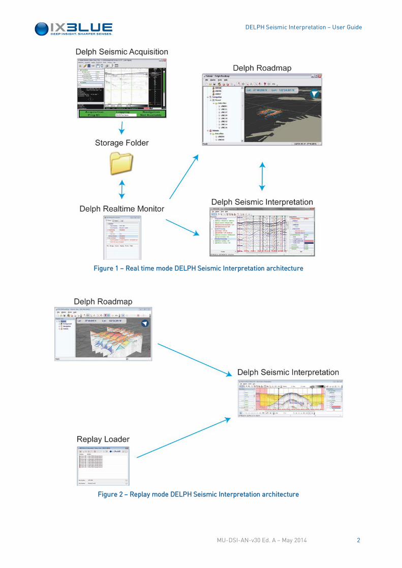
DELPH Seismic Interpretation is a set of software that allows you, both in real time and
replay modes, to (see Figure 1 and Figure 2):
• Access data real time and post-processing (DELPH Real Time Monitor software,
DELPH RoadMap software, DELPH Seismic Replay Loader module)
• Process data (DELPH Seismic Interpretation software)
• Display data (DELPH RoadMap)
Application
Benefits
Survey Strategies
Architecture
MU-DSI-AN-v30 Ed. A – May 2014 1
DELPH Seismic Interpretation – User Guide
Figure 1 – Real time mode DELPH Seismic Interpretation architecture
Figure 2 – Replay mode DELPH Seismic Interpretation architecture
MU-DSI-AN-v30 Ed. A – May 2014 2

DELPH Seismic Interpretation – User Guide
Raw data consists in:
• Seismic signal data, acquired simultaneously or not, during a survey along survey lines
(where Profiles are generated).
• Vessel navigation data.
Once data has been processed, bottom and reflectors can be tracked.
Then the crossings can be computed and Digital Terrain Models (DTM) can be built.
All along the various processing, processed data can be visualized, printed and exported.
Geo-referenced images of the seismic profile are displayed as GeoSections in DELPH
RoadMap.
MU-DSI-AN-v30 Ed. A – May 2014 3
DELPH Seismic Interpretation – User Guide
II GETTING STARTED WITH DELPH SEISMIC INTERPRETATION
II.1 System Requirements
The minimum PC configuration must be: • An Intel Pentium® IV or faster CPU running on a Microsoft® Windows®-based
computer (Windows® XP Service pack 2 minimum)
• 512 MB of RAM for data logging, 1 GB as minimum for full interpretation package
(excluding the memory required by the operating system)
• 500 MB of disk space for installation files
• Enough storage space to hold all data
• 3D Graphical board supporting OpenGL for DELPH RoadMap application
The standard PC configuration is:
• Intel Core 2 Duo @ 3 GHz CPU running on a Microsoft® Windows®-based computer
(Windows® XP Service pack 2 minimum)
• 4 GB of RAM for the complete interpretation package
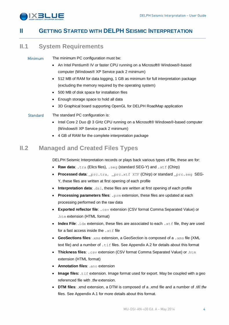
II.2 Managed and Created Files Types
DELPH Seismic Interpretation records or plays back various types of file, these are for:
• Raw data: .tra (Elics files), .seg (standard SEG-Y) and .xtf (Chirp)
• Processed data: _prc.tra, _prc.xtf XTF (Chirp) or standard _prc.seg SEG-
Y, these files are written at first opening of each profile
• Interpretation data: .dsi, these files are written at first opening of each profile
• Processing parameters files: .prm extension, these files are updated at each
processing performed on the raw data
• Exported reflector file: .csv extension (CSV format Comma Separated Value) or
.htm extension (HTML format)
• Index File: .idx extension, these files are associated to each .xtf file, they are used
for a fast access inside the .xtf file
• GeoSections files: .xms extension, a GeoSection is composed of a .xms file (XML
text file) and a number of .tif files. See Appendix A.2 for details about this format
• Thickness files: .csv extension (CSV format Comma Separated Value) or .htm
extension (HTML format)
• Annotation files: .ano extension
• Image files: .tif extension. Image format used for export. May be coupled with a geo
referenced file with .tfw extension.
• DTM files: .xmd extension, a DTM is composed of a .xmd file and a number of .tif/.tfw
files. See Appendix A.1 for more details about this format.
Minimum
Standard
MU-DSI-AN-v30 Ed. A – May 2014 4
DELPH Seismic Interpretation – User Guide
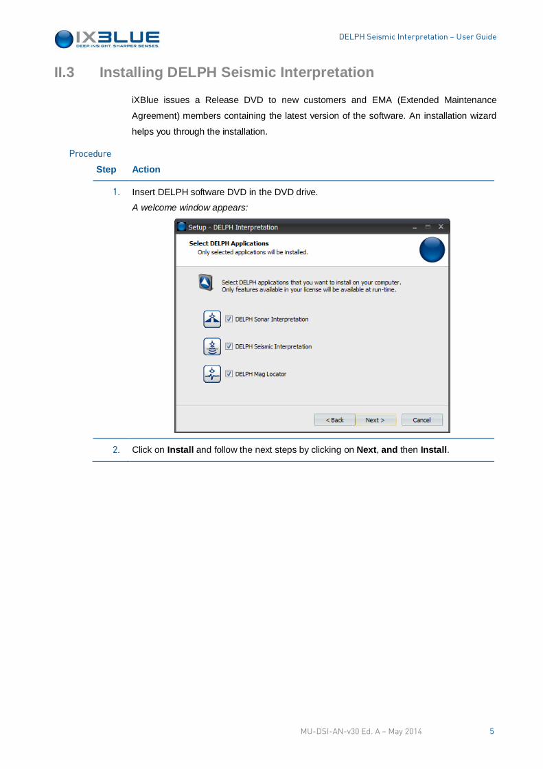
II.3 Installing DELPH Seismic Interpretation
iXBlue issues a Release DVD to new customers and EMA (Extended Maintenance
Agreement) members containing the latest version of the software. An installation wizard
helps you through the installation.
Step Action
1. Insert DELPH software DVD in the DVD drive.
A welcome window appears:
2. Click on Install and follow the next steps by clicking on Next, and then Install.
Procedure
MU-DSI-AN-v30 Ed. A – May 2014 5
DELPH Seismic Interpretation – User Guide
Step Action
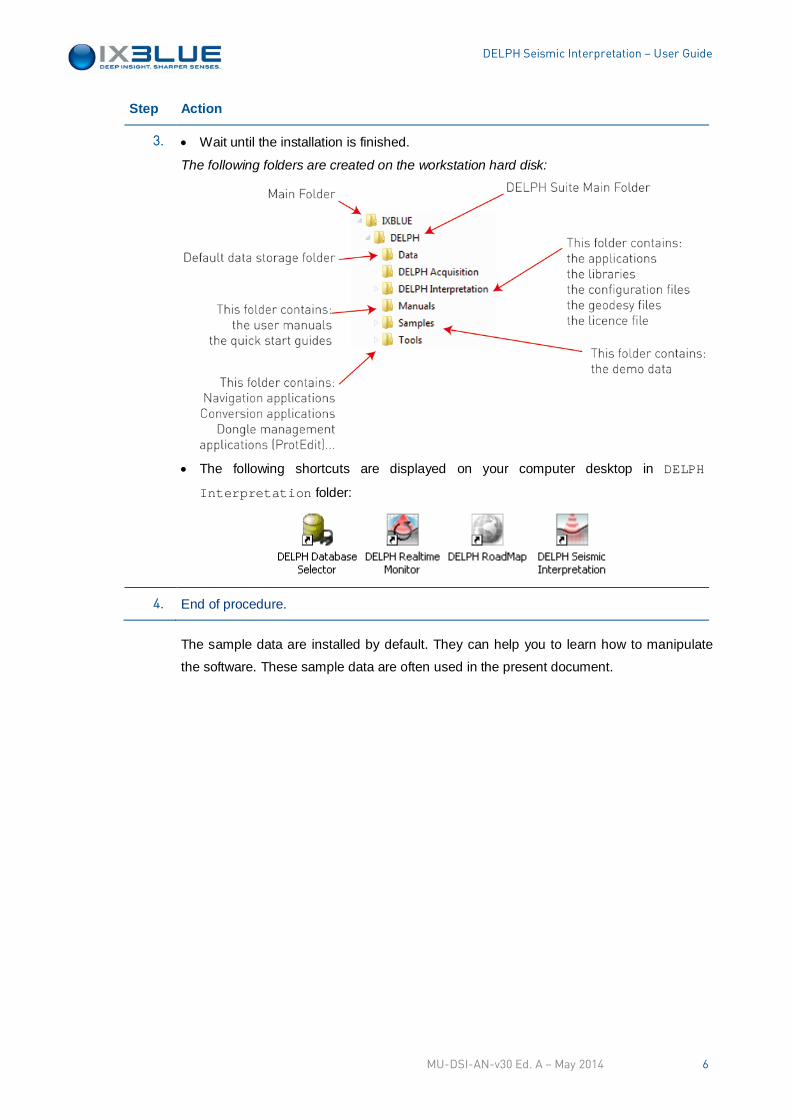
3. • Wait until the installation is finished.
The following folders are created on the workstation hard disk:
• The following shortcuts are displayed on your computer desktop in DELPH
Interpretation folder:
4. End of procedure.
The sample data are installed by default. They can help you to learn how to manipulate
the software. These sample data are often used in the present document.
MU-DSI-AN-v30 Ed. A – May 2014 6
DELPH Seismic Interpretation – User Guide
II.4 Service Pack
In addition to the Release DVD, Service Packs are periodically released to fix bugs and
add features reported or requested by users. In such a case, iXBlue provides to you a
Service Pack DVD.
Do not remove DELPH software from your computer before installing the service pack.
Procedure
Step Action
1. Open the DVD main folder.
You find a release note .pdf file and a service pack folder (its name depends of the
software package).
2. Read the release notes .pdf file.
3. Copy the files from the service pack folder to your DELPH folder.
The service pack is now operating.
4. End of procedure.
MU-DSI-AN-v30 Ed. A – May 2014 7
DELPH Seismic Interpretation – User Guide
II.5 Managing License
iXBlue software products are protected by two different means:
• The product uses a file protection if the product has been lent for demonstration
purpose.
• The type of protection is a dongle protection if the product has been purchased.
II.5.1 FILE PROTECTION
The file protection concerns the demonstration version of the software. It offers full access
to all functionalities of the software. The demonstration version is available only for a time
period only that may be extended with the agreement of the manufacturer.
The file protection is based on a license file iXBlue.lic that is given to the customer.
This file should be placed in the DELPH Interpretation folder (default:
C:\IXBLUE\DELPH\DELPH Interpretation).
The extension of a demonstration period is possible with the help of an application
provided with the product. This application is named LicenceEditor.exe. It is located
in DELPH Interpretation folder (default: C:\IXBLUE\DELPH\DELPH Interpretation).
Figure 3 – License Editor Application Logo
If you requested a validity extension, a procedure to apply the validity extension is also
provided.
When an extension has already been made to the original validity period, de-installing and
re-installing DELPH suite will result in the need of the generation of a new activation key
by iXBlue.
Principle
Demonstration Period
Extension
MU-DSI-AN-v30 Ed. A – May 2014 8
DELPH Seismic Interpretation – User Guide
II.5.2 DONGLE PROTECTION
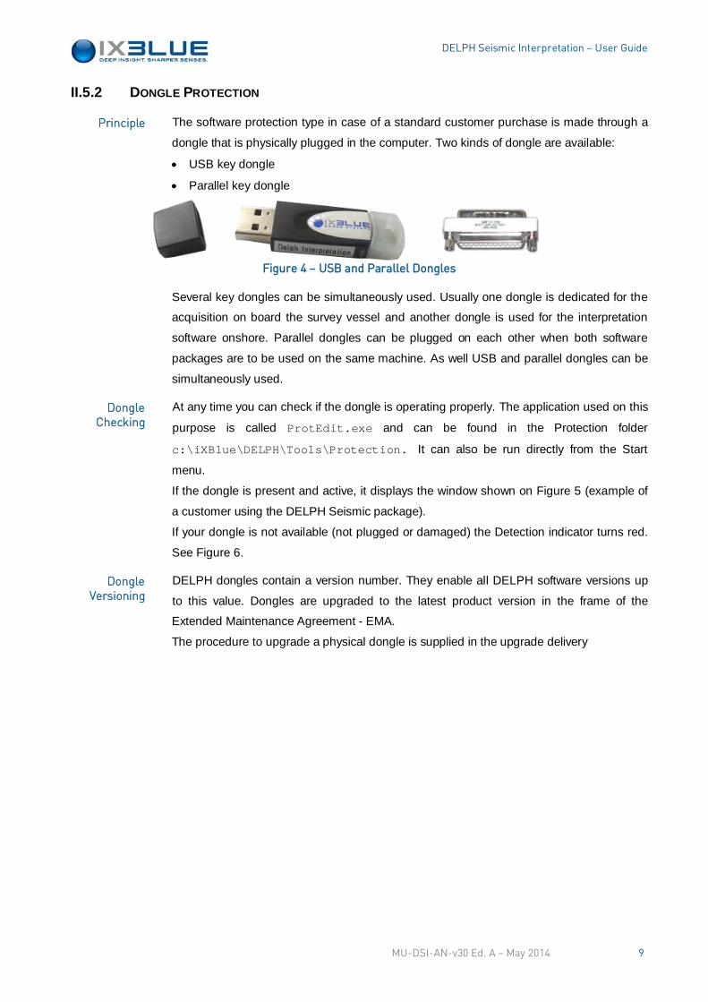
The software protection type in case of a standard customer purchase is made through a
dongle that is physically plugged in the computer. Two kinds of dongle are available:
• USB key dongle
• Parallel key dongle
Figure 4 – USB and Parallel Dongles
Several key dongles can be simultaneously used. Usually one dongle is dedicated for the
acquisition on board the survey vessel and another dongle is used for the interpretation
software onshore. Parallel dongles can be plugged on each other when both software
packages are to be used on the same machine. As well USB and parallel dongles can be
simultaneously used.
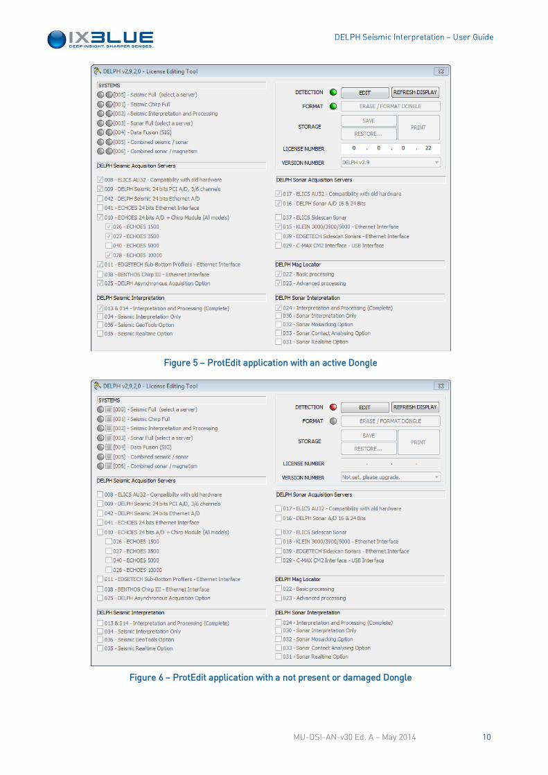
At any time you can check if the dongle is operating properly. The application used on this
purpose is called ProtEdit.exe and can be found in the Protection folder
c:\iXBlue\DELPH\Tools\Protection. It can also be run directly from the Start
menu.
If the dongle is present and active, it displays the window shown on Figure 5 (example of
a customer using the DELPH Seismic package).
If your dongle is not available (not plugged or damaged) the Detection indicator turns red.
See Figure 6.
DELPH dongles contain a version number. They enable all DELPH software versions up
to this value. Dongles are upgraded to the latest product version in the frame of the
Extended Maintenance Agreement - EMA.
The procedure to upgrade a physical dongle is supplied in the upgrade delivery
Principle
Dongle Checking
Dongle Versioning
MU-DSI-AN-v30 Ed. A – May 2014 9
DELPH Seismic Interpretation – User Guide
Figure 5 – ProtEdit application with an active Dongle
Figure 6 – ProtEdit application with a not present or damaged Dongle
MU-DSI-AN-v30 Ed. A – May 2014 10
DELPH Seismic Interpretation – User Guide
III MANAGING A PROJECT
III.1 Introduction
A number of preliminary steps are required to ensure that all survey data is stored in a
consistent file structure that can be archived or shared between users later on. A project
database is created and used by all DELPH Interpretation software to establish the
relationships between the raw data files and interpreted information. This mainly concerns
sonar contacts, and sub-bottom data interpretation. As an example, the database contains
all sonar contacts types in use for a project so that a same classification list is proposed
throughout the survey interpretation. As well, this database contains the sub-bottom
reflectors list that is synchronized at any step of the interpretation.
At the first opening of the survey data records, DELPH computes a processed navigation
to eliminate bad positions and interpolates the navigation to assign a position to each
ping. This navigation processing includes the compensation from the sensor geometry
that is defined by the offsets between the sensors in use.
III.2 Project File Structure
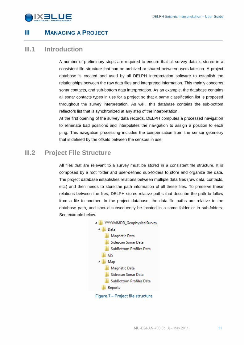
All files that are relevant to a survey must be stored in a consistent file structure. It is
composed by a root folder and user-defined sub-folders to store and organize the data.
The project database establishes relations between multiple data files (raw data, contacts,
etc.) and then needs to store the path information of all these files. To preserve these
relations between the files, DELPH stores relative paths that describe the path to follow
from a file to another. In the project database, the data file paths are relative to the
database path, and should subsequently be located in a same folder or in sub-folders.
See example below.
Figure 7 – Project file structure
MU-DSI-AN-v30 Ed. A – May 2014 11
DELPH Seismic Interpretation – User Guide
III.3 Creating or Selecting a Project Database
Interpretation data that is shared among profiles like side-scan sonar contacts and their
classification attributes, measurements, etc. is managed in a relational database. At the
beginning of a work session, check that the proper project database is selected if not
select or create another one. An application named DELPH Database Selector provides
commands to create and select project databases. It also provides a visualization of data
files that are referenced. Please note that a project database uses relative paths to the
data files. Then it is highly recommended to store it at the root of the project file structure.
Figure 8 – DELPH Database Selector icon
Step Action
1. Close all DELPH applications currently running. Launch DELPH Database Selector.
The main window of the application opens.
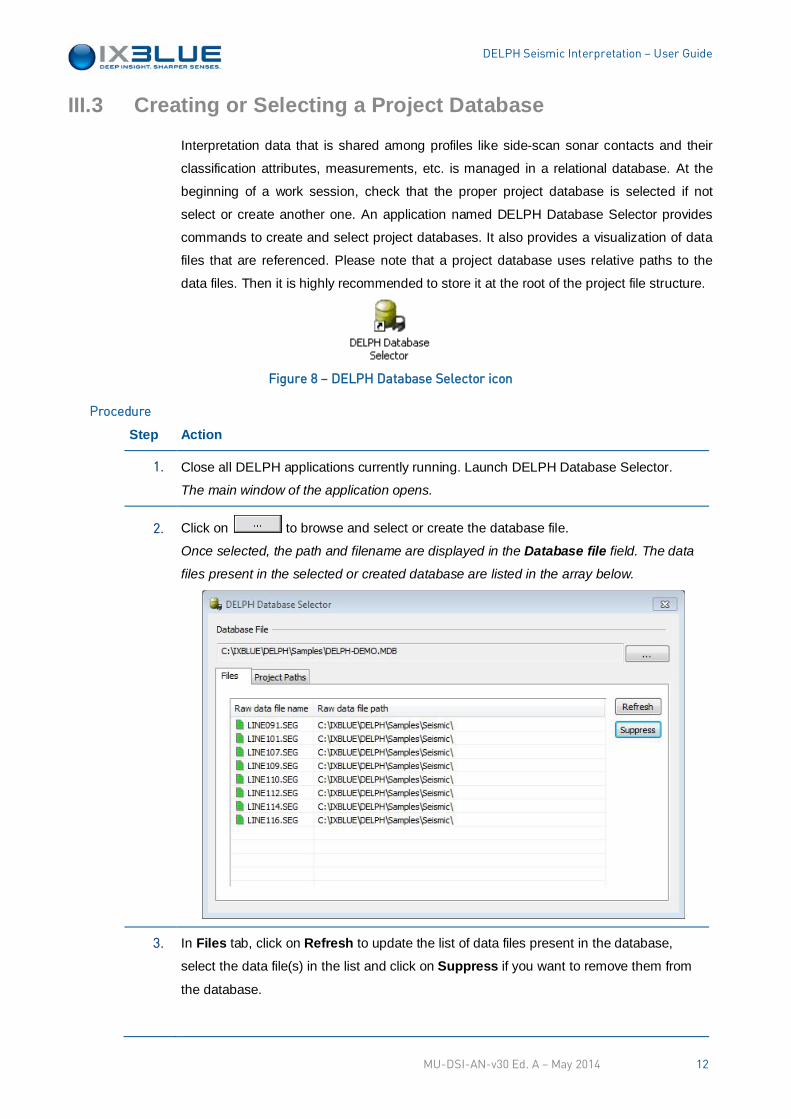
2. Click on to browse and select or create the database file.
Once selected, the path and filename are displayed in the Database file field. The data
files present in the selected or created database are listed in the array below.
3. In Files tab, click on Refresh to update the list of data files present in the database,
select the data file(s) in the list and click on Suppress if you want to remove them from
the database.
Procedure
MU-DSI-AN-v30 Ed. A – May 2014 12
DELPH Seismic Interpretation – User Guide
Step Action
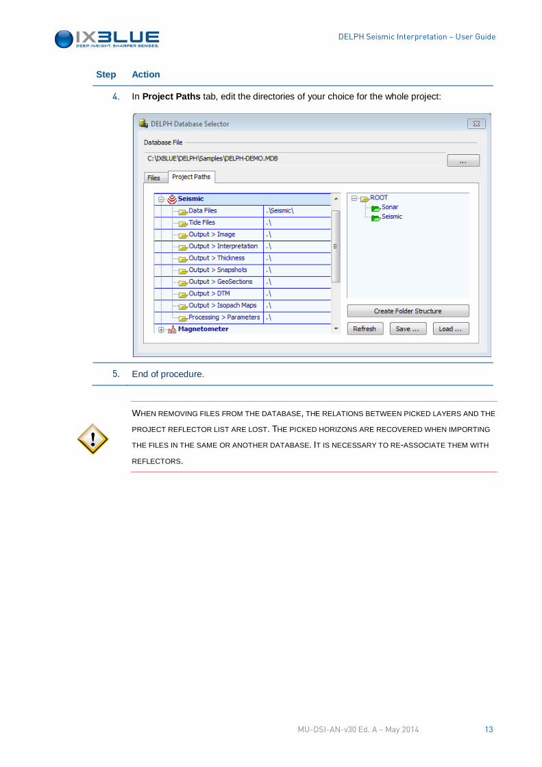
4. In Project Paths tab, edit the directories of your choice for the whole project:
5. End of procedure.
WHEN REMOVING FILES FROM THE DATABASE, THE RELATIONS BETWEEN PICKED LAYERS AND THE
PROJECT REFLECTOR LIST ARE LOST. THE PICKED HORIZONS ARE RECOVERED WHEN IMPORTING
THE FILES IN THE SAME OR ANOTHER DATABASE. IT IS NECESSARY TO RE-ASSOCIATE THEM WITH
REFLECTORS.
MU-DSI-AN-v30 Ed. A – May 2014 13
DELPH Seismic Interpretation – User Guide
III.4 Using an Geometry File from DELPH Acquisition
The sensor geometry is defined during the acquisition in the DELPH Acquisition software.
DELPH Acquisition keeps track of the sensor geometry configuration in the file named
"DelphSeismic.GEO". This file is stored in the default DELPH data folder
(C:\IXBLUE\DELPH\Data). This file contains all the offsets to integrate when computing
the sensor navigation. This file is opened at the same time as the XTF file in the DELPH
Interpretation software. After processing, a new geometry file is created and stored in the
folder of the corresponding processed XTF files. The geometry parameters are extracted
from the following files which are listed in priority order:
• Geometry file associated to the XTF file
• Geometry file associated to the storage folder of the XTF files
• Geometry file stored in the raw folder /DATA
The geometry files are written in ASCII format using the XML syntax. This structure
contains various entries:
<geometry/> // Geometry file section
<mobile/> // Mobile section (i.e. Vessel)
<equipment name="GPS"> // GPS offset description
<mount/> // GPS mounting type
<offset/> // GPS offsets
</equipment> // End of GPS description
<equipment name="MRU"/> // Motion Reference Unit description
<equipment name="Winch"/> // Winch / Tow point description
<equipment name="Seismic"/> // System description
</mobile> // End of the mobile section
</geometry> // End of the geometry file section
When using DELPH Sonar Interpretation on a same PC as DELPH Acquisition, the
geometry file is shared between both applications.
When using DELPH Interpretation in standalone mode, either the geometry file must be
copied from DELPH Acquisition workstation, or they must be manually edited.
Alternatively, DELPH uses the offsets that can be found in the seismic records, or a
"DelphSeismic.GEO" file that is located in the XTF data folder.
The geometry settings are editable, see section V.3.3.
MU-DSI-AN-v30 Ed. A – May 2014 14
DELPH Seismic Interpretation – User Guide
IV DELPH ROADMAP
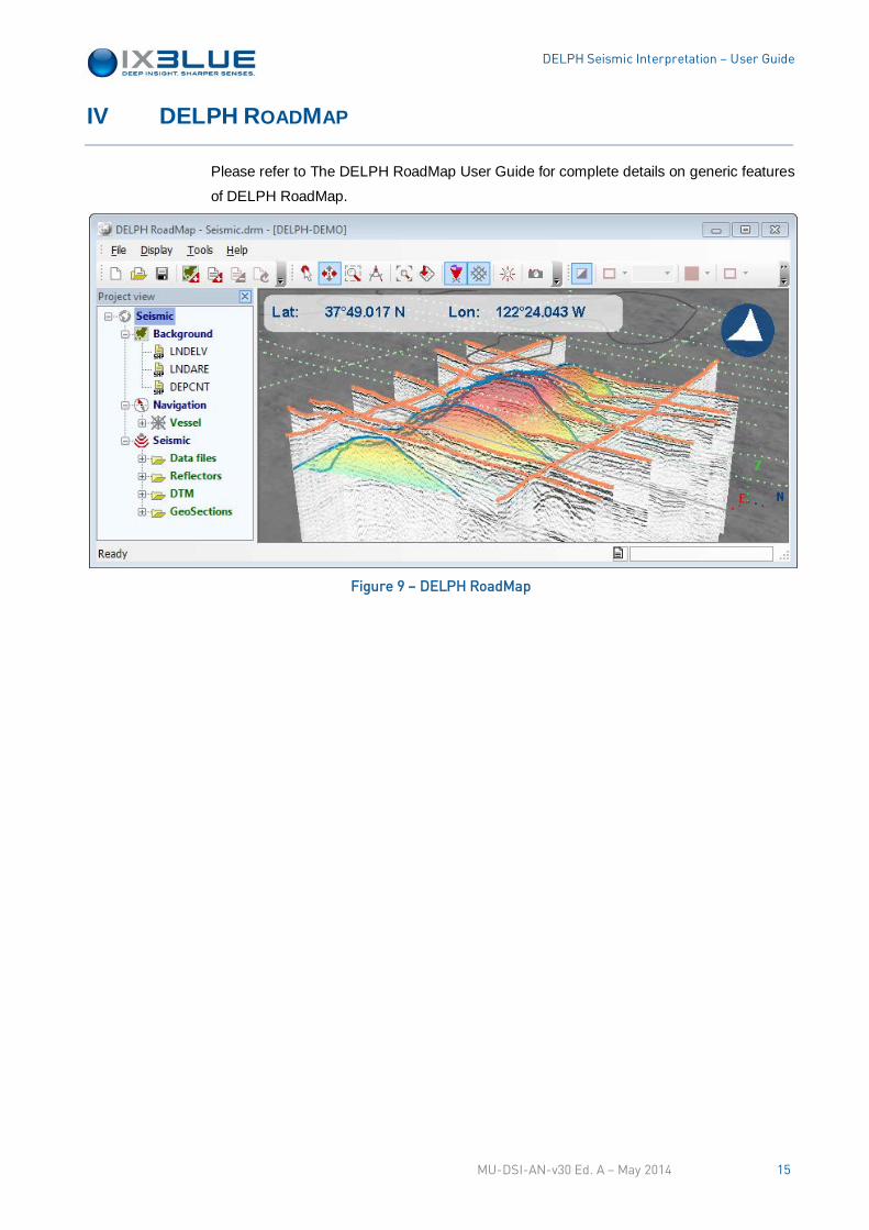
Please refer to The DELPH RoadMap User Guide for complete details on generic features
of DELPH RoadMap.
Figure 9 – DELPH RoadMap
MU-DSI-AN-v30 Ed. A – May 2014 15
DELPH Seismic Interpretation – User Guide
V DELPH SEISMIC INTERPRETATION
V.1 Introduction
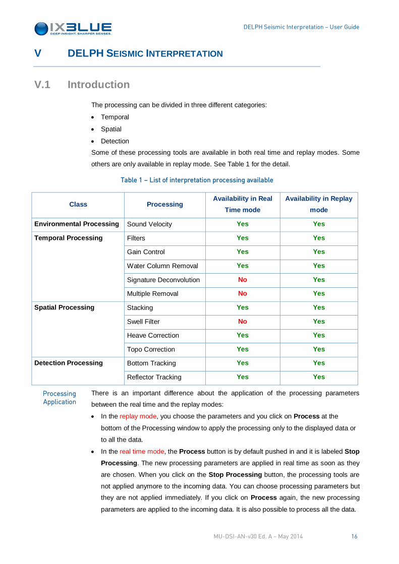
The processing can be divided in three different categories:
• Temporal
• Spatial
• Detection
Some of these processing tools are available in both real time and replay modes. Some
others are only available in replay mode. See Table 1 for the detail.
Table 1 – List of interpretation processing available
Class Processing Availability in Real
Time mode Availability in Replay
mode
Environmental Processing Sound Velocity Yes Yes
Temporal Processing Filters Yes Yes
Gain Control Yes Yes
Water Column Removal Yes Yes
Signature Deconvolution No Yes
Multiple Removal No Yes
Spatial Processing Stacking Yes Yes
Swell Filter No Yes
Heave Correction Yes Yes
Topo Correction Yes Yes
Detection Processing Bottom Tracking Yes Yes
Reflector Tracking Yes Yes
There is an important difference about the application of the processing parameters
between the real time and the replay modes:
• In the replay mode, you choose the parameters and you click on Process at the
bottom of the Processing window to apply the processing only to the displayed data or
to all the data.
• In the real time mode, the Process button is by default pushed in and it is labeled Stop Processing. The new processing parameters are applied in real time as soon as they
are chosen. When you click on the Stop Processing button, the processing tools are
not applied anymore to the incoming data. You can choose processing parameters but
they are not applied immediately. If you click on Process again, the new processing
parameters are applied to the incoming data. It is also possible to process all the data.
Processing Application
MU-DSI-AN-v30 Ed. A – May 2014 16
DELPH Seismic Interpretation – User Guide
V.1.1 REAL TIME MODE
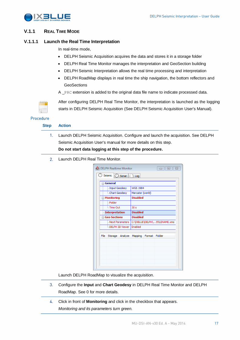
V.1.1.1 Launch the Real Time Interpretation In real-time mode,
• DELPH Seismic Acquisition acquires the data and stores it in a storage folder
• DELPH Real Time Monitor manages the interpretation and GeoSection building
• DELPH Seismic Interpretation allows the real time processing and interpretation
• DELPH RoadMap displays in real time the ship navigation, the bottom reflectors and
GeoSections
A _PRC extension is added to the original data file name to indicate processed data.
After configuring DELPH Real Time Monitor, the interpretation is launched as the logging
starts in DELPH Seismic Acquisition (See DELPH Seismic Acquisition User’s Manual).
Step Action
1. Launch DELPH Seismic Acquisition. Configure and launch the acquisition. See DELPH
Seismic Acquisition User’s manual for more details on this step.
Do not start data logging at this step of the procedure.
2. Launch DELPH Real Time Monitor.
Launch DELPH RoadMap to visualize the acquisition.
3. Configure the Input and Chart Geodesy in DELPH Real Time Monitor and DELPH
RoadMap. See 0 for more details.
4. Click in front of Monitoring and click in the checkbox that appears.
Monitoring and its parameters turn green.
Procedure
MU-DSI-AN-v30 Ed. A – May 2014 17
DELPH Seismic Interpretation – User Guide
Step Action
5. Click in front of Folder. Click on to browse for the folder where DELPH Seismic
Acquisition stores the data.
Enter a Time Out value (the time with no update in the file and after which the software
considers the file as terminated and looks for another file).
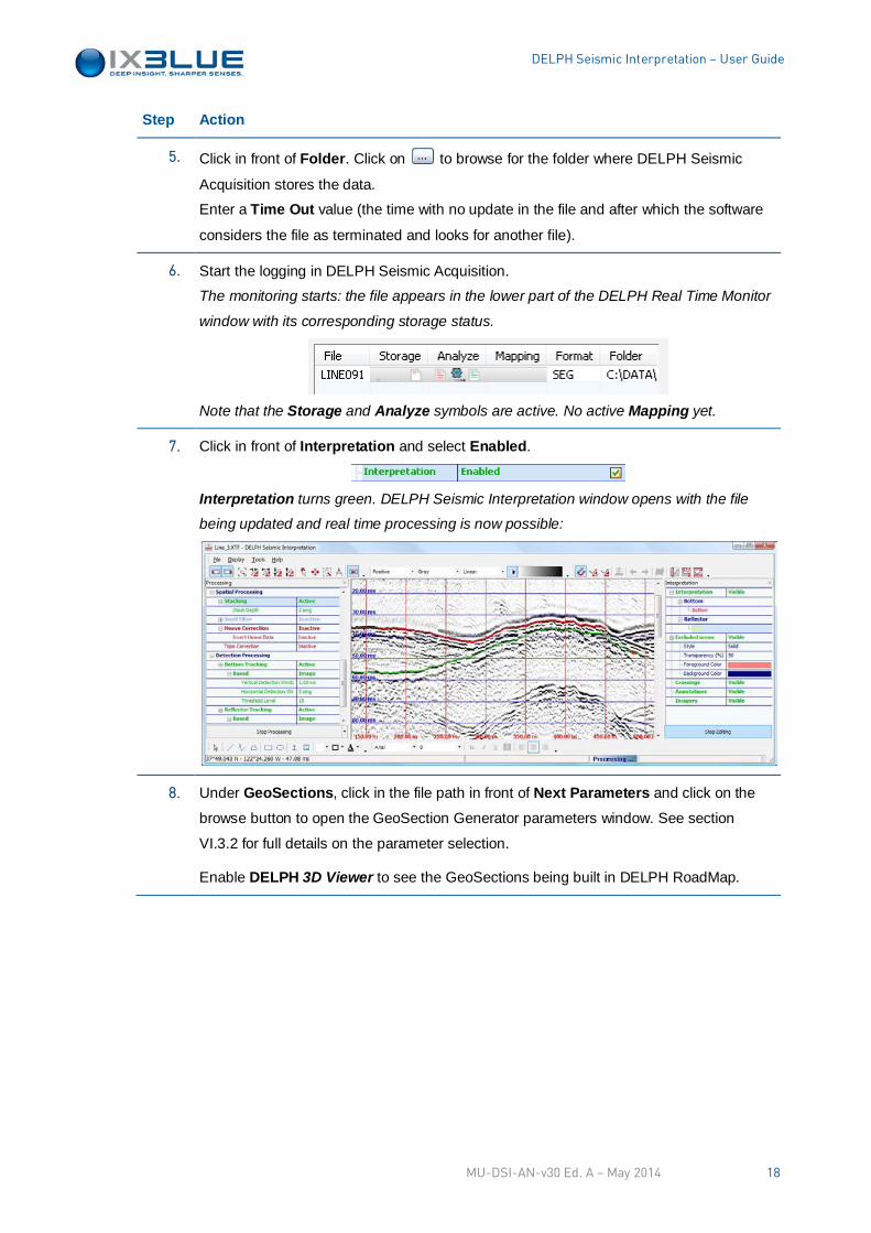
6. Start the logging in DELPH Seismic Acquisition.
The monitoring starts: the file appears in the lower part of the DELPH Real Time Monitor
window with its corresponding storage status.
Note that the Storage and Analyze symbols are active. No active Mapping yet.
7. Click in front of Interpretation and select Enabled.
Interpretation turns green. DELPH Seismic Interpretation window opens with the file
being updated and real time processing is now possible:
8. Under GeoSections, click in the file path in front of Next Parameters and click on the
browse button to open the GeoSection Generator parameters window. See section
VI.3.2 for full details on the parameter selection.
Enable DELPH 3D Viewer to see the GeoSections being built in DELPH RoadMap.
MU-DSI-AN-v30 Ed. A – May 2014 18
DELPH Seismic Interpretation – User Guide
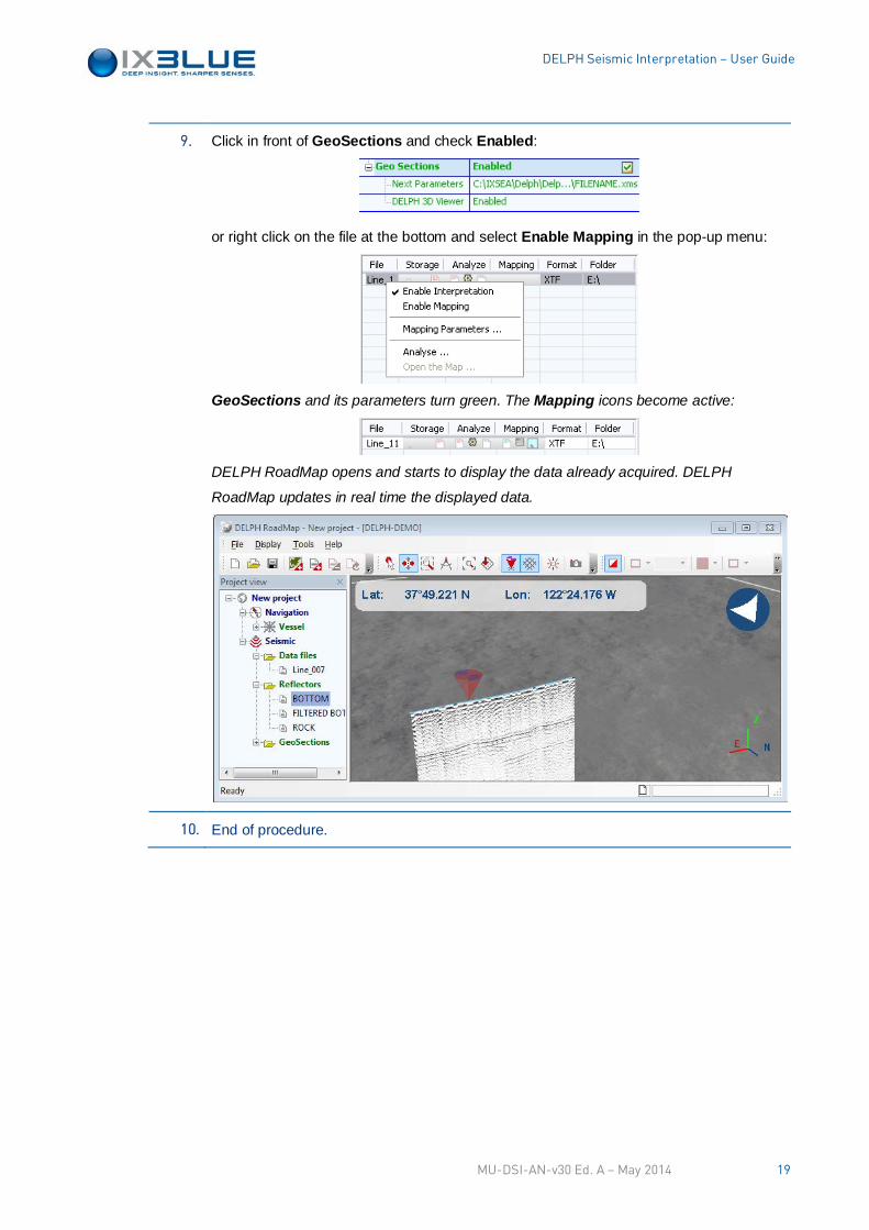
9. Click in front of GeoSections and check Enabled:
or right click on the file at the bottom and select Enable Mapping in the pop-up menu:
GeoSections and its parameters turn green. The Mapping icons become active:
DELPH RoadMap opens and starts to display the data already acquired. DELPH
RoadMap updates in real time the displayed data.
10. End of procedure.
MU-DSI-AN-v30 Ed. A – May 2014 19
DELPH Seismic Interpretation – User Guide
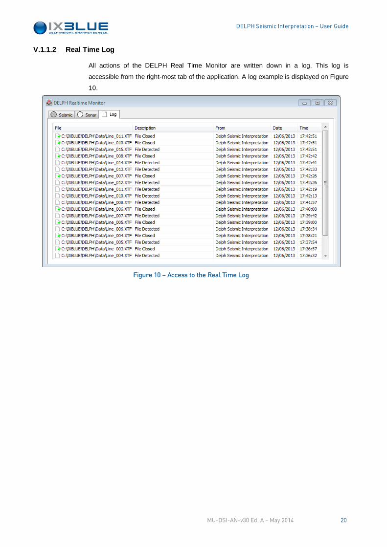
V.1.1.2 Real Time Log
All actions of the DELPH Real Time Monitor are written down in a log. This log is
accessible from the right-most tab of the application. A log example is displayed on Figure
10.
Figure 10 – Access to the Real Time Log
MU-DSI-AN-v30 Ed. A – May 2014 20
DELPH Seismic Interpretation – User Guide
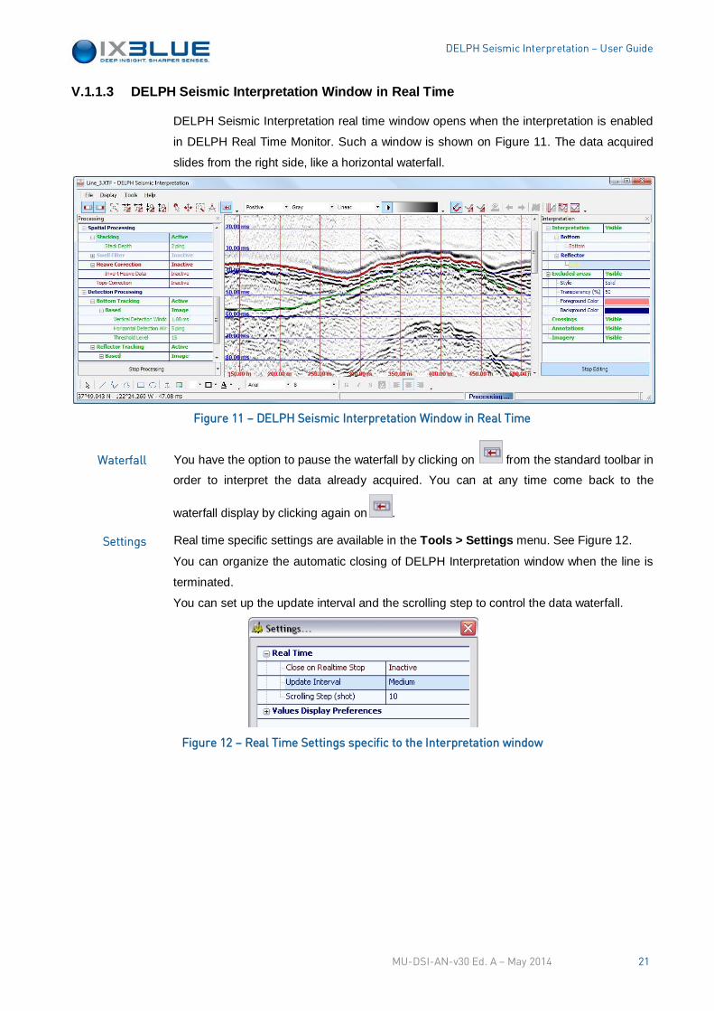
V.1.1.3 DELPH Seismic Interpretation Window in Real Time
DELPH Seismic Interpretation real time window opens when the interpretation is enabled
in DELPH Real Time Monitor. Such a window is shown on Figure 11. The data acquired
slides from the right side, like a horizontal waterfall.
Figure 11 – DELPH Seismic Interpretation Window in Real Time
You have the option to pause the waterfall by clicking on from the standard toolbar in
order to interpret the data already acquired. You can at any time come back to the
waterfall display by clicking again on .
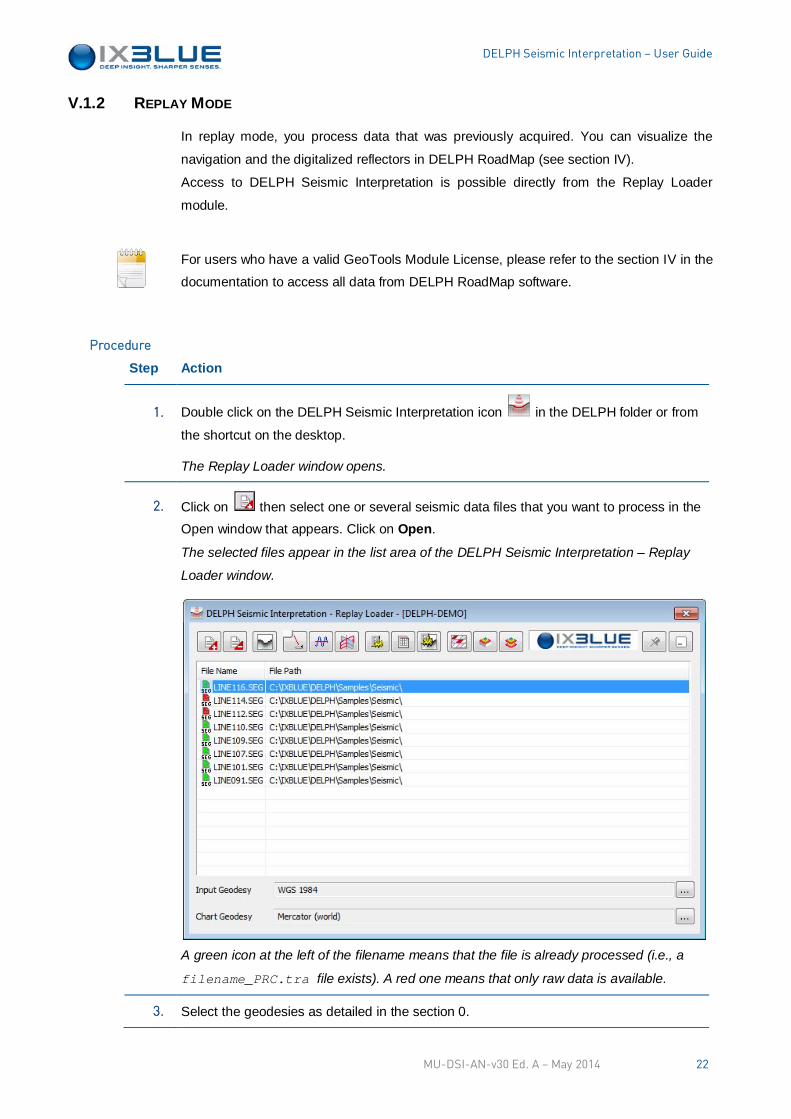
Real time specific settings are available in the Tools > Settings menu. See Figure 12.
You can organize the automatic closing of DELPH Interpretation window when the line is
terminated.
You can set up the update interval and the scrolling step to control the data waterfall.
Figure 12 – Real Time Settings specific to the Interpretation window
Waterfall
Settings
MU-DSI-AN-v30 Ed. A – May 2014 21
DELPH Seismic Interpretation – User Guide
V.1.2 REPLAY MODE
In replay mode, you process data that was previously acquired. You can visualize the
navigation and the digitalized reflectors in DELPH RoadMap (see section IV).
Access to DELPH Seismic Interpretation is possible directly from the Replay Loader
module.
For users who have a valid GeoTools Module License, please refer to the section IV in the
documentation to access all data from DELPH RoadMap software.
Step Action
1. Double click on the DELPH Seismic Interpretation icon in the DELPH folder or from
the shortcut on the desktop.
The Replay Loader window opens.
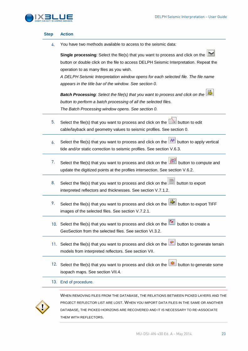
2. Click on then select one or several seismic data files that you want to process in the Open window that appears. Click on Open.
The selected files appear in the list area of the DELPH Seismic Interpretation – Replay
Loader window.
A green icon at the left of the filename means that the file is already processed (i.e., a
filename_PRC.tra file exists). A red one means that only raw data is available.
3. Select the geodesies as detailed in the section 0.
Procedure
MU-DSI-AN-v30 Ed. A – May 2014 22
DELPH Seismic Interpretation – User Guide
Step Action
4. You have two methods available to access to the seismic data:
Single processing: Select the file(s) that you want to process and click on the
button or double click on the file to access DELPH Seismic Interpretation. Repeat the
operation to as many files as you wish.
A DELPH Seismic Interpretation window opens for each selected file. The file name
appears in the title bar of the window. See section 0.
Batch Processing: Select the file(s) that you want to process and click on the
button to perform a batch processing of all the selected files.
The Batch Processing window opens. See section 0.
5. Select the file(s) that you want to process and click on the button to edit
cable/layback and geometry values to seismic profiles. See section 0.
6. Select the file(s) that you want to process and click on the button to apply vertical
tide and/or static correction to seismic profiles. See section V.6.3.
7. Select the file(s) that you want to process and click on the button to compute and
update the digitized points at the profiles intersection. See section V.6.2.
8. Select the file(s) that you want to process and click on the button to export
interpreted reflectors and thicknesses. See section V.7.1.2.
9. Select the file(s) that you want to process and click on the button to export TIFF
images of the selected files. See section V.7.2.1.
10.
Select the file(s) that you want to process and click on the button to create a
GeoSection from the selected files. See section VI.3.2.
11. Select the file(s) that you want to process and click on the button to generate terrain
models from interpreted reflectors. See section VII.
12. Select the file(s) that you want to process and click on the button to generate some
isopach maps. See section VII.4.
13. End of procedure.
WHEN REMOVING FILES FROM THE DATABASE, THE RELATIONS BETWEEN PICKED LAYERS AND THE
PROJECT REFLECTOR LIST ARE LOST. WHEN YOU IMPORT DATA FILES IN THE SAME OR ANOTHER
DATABASE, THE PICKED HORIZONS ARE RECOVERED AND IT IS NECESSARY TO RE-ASSOCIATE
THEM WITH REFLECTORS.
MU-DSI-AN-v30 Ed. A – May 2014 23
DELPH Seismic Interpretation – User Guide
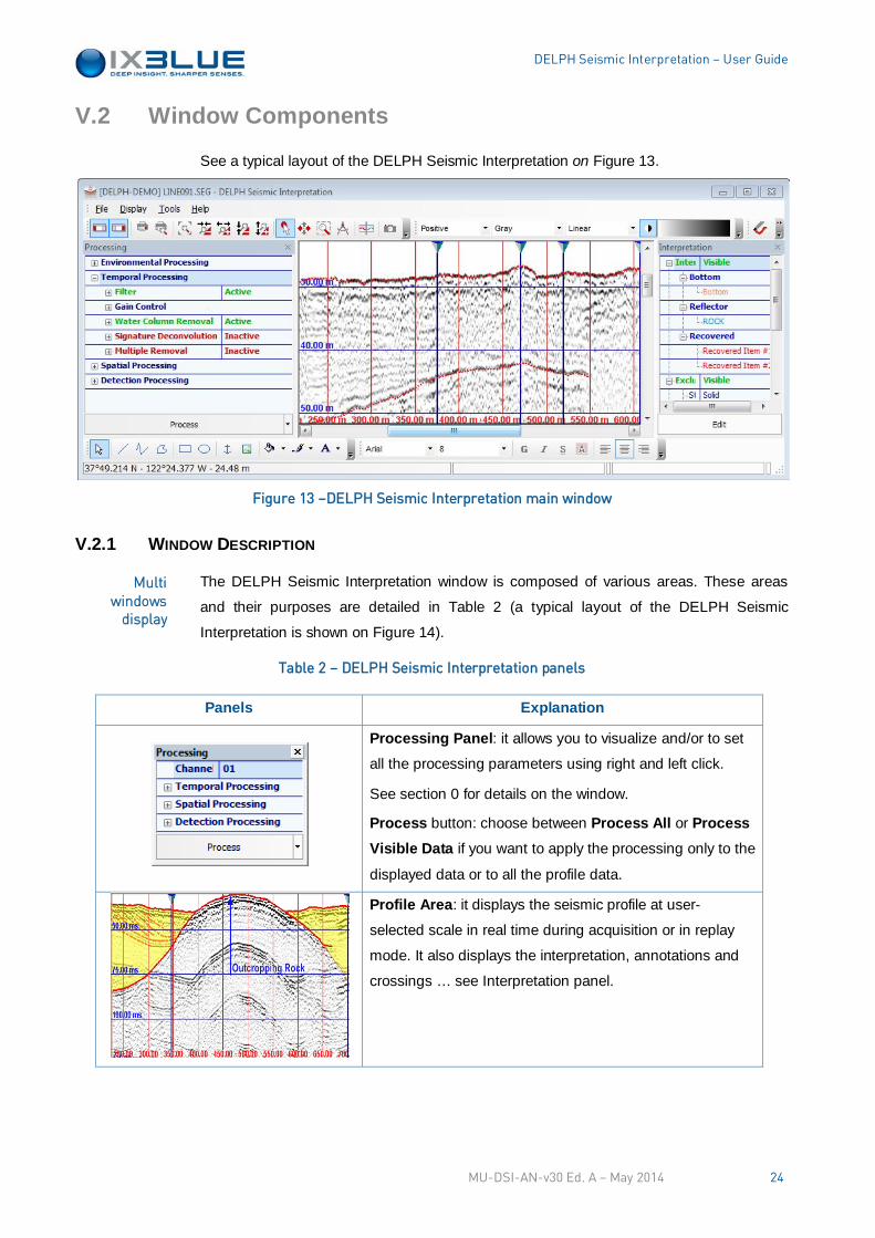
V.2 Window Components
See a typical layout of the DELPH Seismic Interpretation on Figure 13.
Figure 13 –DELPH Seismic Interpretation main window
V.2.1 WINDOW DESCRIPTION
The DELPH Seismic Interpretation window is composed of various areas. These areas
and their purposes are detailed in Table 2 (a typical layout of the DELPH Seismic
Interpretation is shown on Figure 14).
Table 2 – DELPH Seismic Interpretation panels
Panels Explanation
Processing Panel: it allows you to visualize and/or to set
all the processing parameters using right and left click.
See section 0 for details on the window.
Process button: choose between Process All or Process Visible Data if you want to apply the processing only to the
displayed data or to all the profile data.
Profile Area: it displays the seismic profile at user-
selected scale in real time during acquisition or in replay
mode. It also displays the interpretation, annotations and
crossings … see Interpretation panel.
Multi windows
display
MU-DSI-AN-v30 Ed. A – May 2014 24
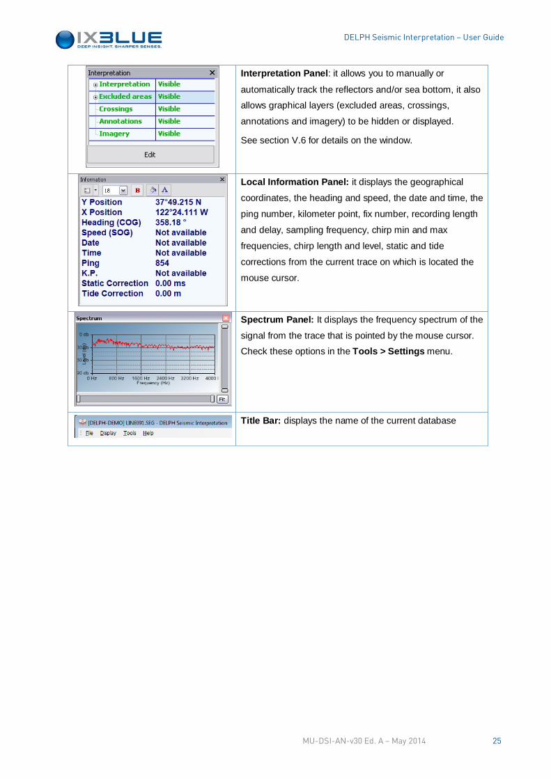
DELPH Seismic Interpretation – User Guide
Interpretation Panel: it allows you to manually or
automatically track the reflectors and/or sea bottom, it also
allows graphical layers (excluded areas, crossings,
annotations and imagery) to be hidden or displayed.
See section V.6 for details on the window.
Local Information Panel: it displays the geographical
coordinates, the heading and speed, the date and time, the
ping number, kilometer point, fix number, recording length
and delay, sampling frequency, chirp min and max
frequencies, chirp length and level, static and tide
corrections from the current trace on which is located the
mouse cursor.
Spectrum Panel: It displays the frequency spectrum of the
signal from the trace that is pointed by the mouse cursor.
Check these options in the Tools > Settings menu.
Title Bar: displays the name of the current database
MU-DSI-AN-v30 Ed. A – May 2014 25
DELPH Seismic Interpretation – User Guide
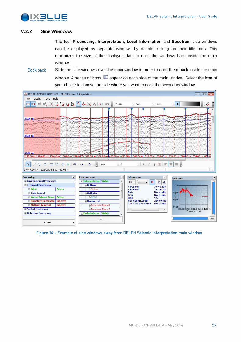
V.2.2 SIDE WINDOWS
The four Processing, Interpretation, Local Information and Spectrum side windows
can be displayed as separate windows by double clicking on their title bars. This
maximizes the size of the displayed data to dock the windows back inside the main
window.
Slide the side windows over the main window in order to dock them back inside the main
window. A series of icons appear on each side of the main window. Select the icon of
your choice to choose the side where you want to dock the secondary window.
Figure 14 – Example of side windows away from DELPH Seismic Interpretation main window
Dock back
MU-DSI-AN-v30 Ed. A – May 2014 26
DELPH Seismic Interpretation – User Guide
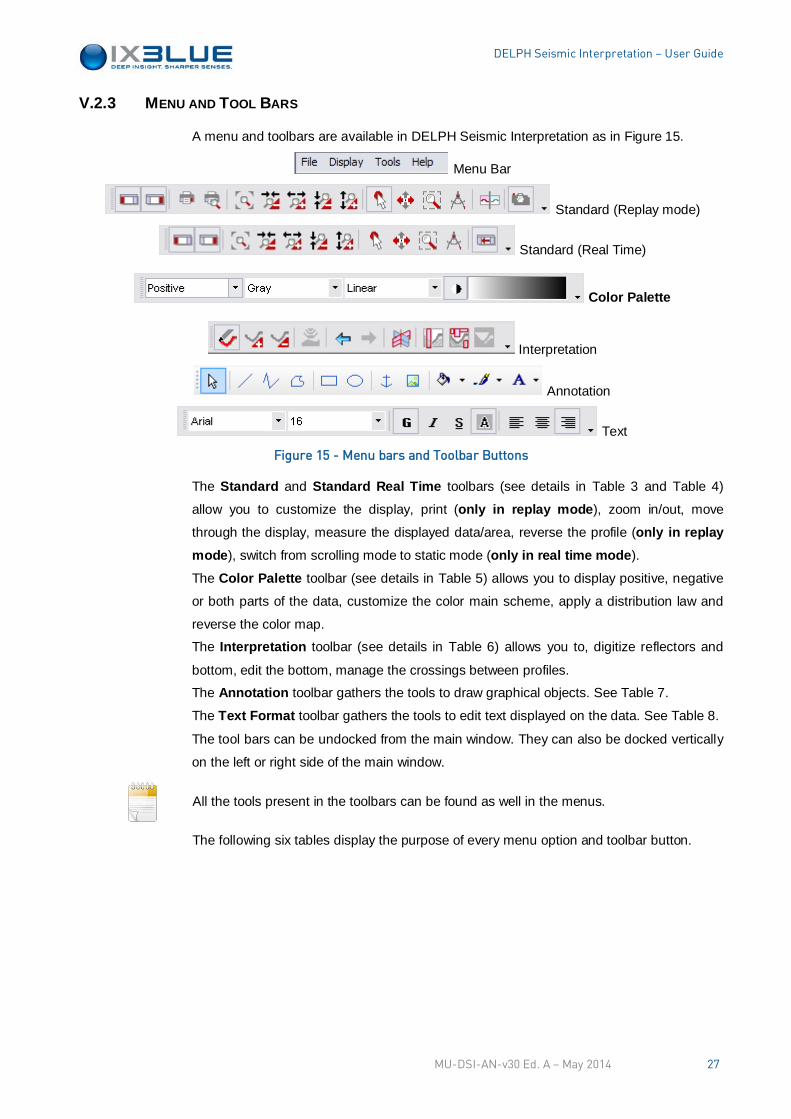
V.2.3 MENU AND TOOL BARS
A menu and toolbars are available in DELPH Seismic Interpretation as in Figure 15.
Menu Bar
Standard (Replay mode)
Standard (Real Time)
Color Palette
Interpretation
Annotation
Text
Figure 15 - Menu bars and Toolbar Buttons
The Standard and Standard Real Time toolbars (see details in Table 3 and Table 4)
allow you to customize the display, print (only in replay mode), zoom in/out, move
through the display, measure the displayed data/area, reverse the profile (only in replay mode), switch from scrolling mode to static mode (only in real time mode).
The Color Palette toolbar (see details in Table 5) allows you to display positive, negative
or both parts of the data, customize the color main scheme, apply a distribution law and
reverse the color map.
The Interpretation toolbar (see details in Table 6) allows you to, digitize reflectors and
bottom, edit the bottom, manage the crossings between profiles.
The Annotation toolbar gathers the tools to draw graphical objects. See Table 7.
The Text Format toolbar gathers the tools to edit text displayed on the data. See Table 8.
The tool bars can be undocked from the main window. They can also be docked vertically
on the left or right side of the main window.
All the tools present in the toolbars can be found as well in the menus.
The following six tables display the purpose of every menu option and toolbar button.
MU-DSI-AN-v30 Ed. A – May 2014 27
DELPH Seismic Interpretation – User Guide
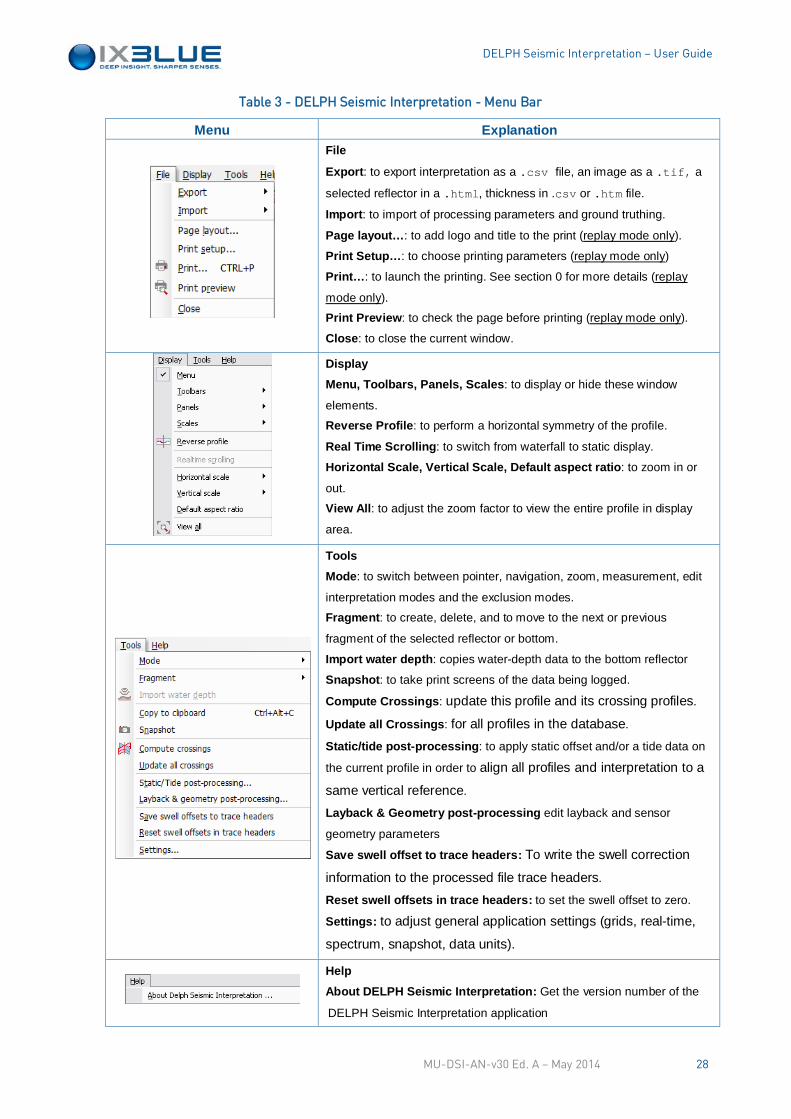
Table 3 - DELPH Seismic Interpretation - Menu Bar
Menu Explanation
File
Export: to export interpretation as a .csv file, an image as a .tif, a
selected reflector in a .html, thickness in .csv or .htm file.
Import: to import of processing parameters and ground truthing.
Page layout…: to add logo and title to the print (replay mode only).
Print Setup…: to choose printing parameters (replay mode only)
Print…: to launch the printing. See section 0 for more details (replay
mode only).
Print Preview: to check the page before printing (replay mode only).
Close: to close the current window.
Display Menu, Toolbars, Panels, Scales: to display or hide these window
elements.
Reverse Profile: to perform a horizontal symmetry of the profile.
Real Time Scrolling: to switch from waterfall to static display.
Horizontal Scale, Vertical Scale, Default aspect ratio: to zoom in or
out.
View All: to adjust the zoom factor to view the entire profile in display
area.
Tools Mode: to switch between pointer, navigation, zoom, measurement, edit
interpretation modes and the exclusion modes.
Fragment: to create, delete, and to move to the next or previous
fragment of the selected reflector or bottom.
Import water depth: copies water-depth data to the bottom reflector
Snapshot: to take print screens of the data being logged.
Compute Crossings: update this profile and its crossing profiles.
Update all Crossings: for all profiles in the database.
Static/tide post-processing: to apply static offset and/or a tide data on
the current profile in order to align all profiles and interpretation to a
same vertical reference.
Layback & Geometry post-processing edit layback and sensor
geometry parameters
Save swell offset to trace headers: To write the swell correction
information to the processed file trace headers.
Reset swell offsets in trace headers: to set the swell offset to zero.
Settings: to adjust general application settings (grids, real-time,
spectrum, snapshot, data units).
Help About DELPH Seismic Interpretation: Get the version number of the
DELPH Seismic Interpretation application
MU-DSI-AN-v30 Ed. A – May 2014 28
DELPH Seismic Interpretation – User Guide
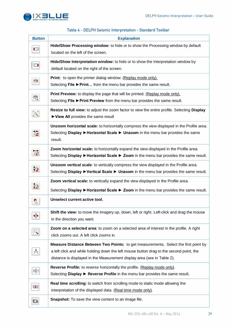
Table 4 - DELPH Seismic Interpretation - Standard Toolbar
Button Explanation
Hide/Show Processing window: to hide or to show the Processing window by default
located on the left of the screen.
Hide/Show Interpretation window: to hide or to show the Interpretation window by
default located on the right of the screen.
Print: to open the printer dialog window. (Replay mode only).
Selecting File ►Print… from the menu bar provides the same result.
Print Preview: to display the page that will be printed. (Replay mode only).
Selecting File ►Print Preview from the menu bar provides the same result.
Resize to full view: to adjust the zoom factor to view the entire profile. Selecting Display ►View All provides the same result
Unzoom horizontal scale: to horizontally compress the view displayed in the Profile area.
Selecting Display ►Horizontal Scale ► Unzoom in the menu bar provides the same
result.
Zoom horizontal scale: to horizontally expand the view displayed in the Profile area.
Selecting Display ►Horizontal Scale ► Zoom in the menu bar provides the same result.
Unzoom vertical scale: to vertically compress the view displayed in the Profile area.
Selecting Display ►Vertical Scale ► Unzoom in the menu bar provides the same result.
Zoom vertical scale: to vertically expand the view displayed in the Profile area.
Selecting Display ►Horizontal Scale ► Zoom in the menu bar provides the same result.
Unselect current active tool.
Shift the view: to move the imagery up, down, left or right. Left-click and drag the mouse
in the direction you want.
Zoom on a selected area: to zoom on a selected area of interest in the profile. A right
click zooms out. A left click zooms in.
Measure Distance Between Two Points: to get measurements. Select the first point by
a left click and while holding down the left mouse button drag to the second point, the
distance is displayed in the Measurement display area (see in Table 2).
Reverse Profile: to reverse horizontally the profile. (Replay mode only).
Selecting Display ► Reverse Profile in the menu bar provides the same result.
Real time scrolling: to switch from scrolling mode to static mode allowing the
interpretation of the displayed data. (Real time mode only).
Snapshot: To save the view content to an image file.
MU-DSI-AN-v30 Ed. A – May 2014 29
DELPH Seismic Interpretation – User Guide
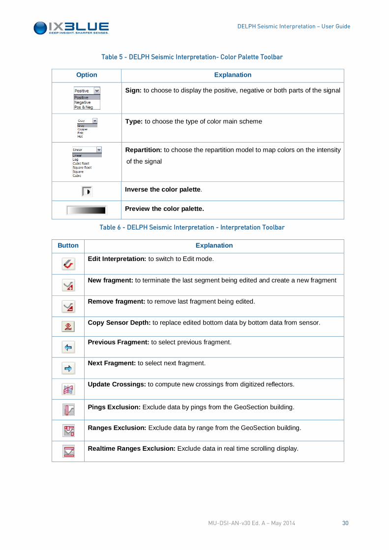
Table 5 - DELPH Seismic Interpretation- Color Palette Toolbar
Option Explanation
Sign: to choose to display the positive, negative or both parts of the signal
Type: to choose the type of color main scheme
Repartition: to choose the repartition model to map colors on the intensity
of the signal
Inverse the color palette.
Preview the color palette.
Table 6 - DELPH Seismic Interpretation - Interpretation Toolbar
Button Explanation
Edit Interpretation: to switch to Edit mode.
New fragment: to terminate the last segment being edited and create a new fragment
Remove fragment: to remove last fragment being edited.
Copy Sensor Depth: to replace edited bottom data by bottom data from sensor.
Previous Fragment: to select previous fragment.
Next Fragment: to select next fragment.
Update Crossings: to compute new crossings from digitized reflectors.
Pings Exclusion: Exclude data by pings from the GeoSection building.
Ranges Exclusion: Exclude data by range from the GeoSection building.
Realtime Ranges Exclusion: Exclude data in real time scrolling display.
MU-DSI-AN-v30 Ed. A – May 2014 30
DELPH Seismic Interpretation – User Guide
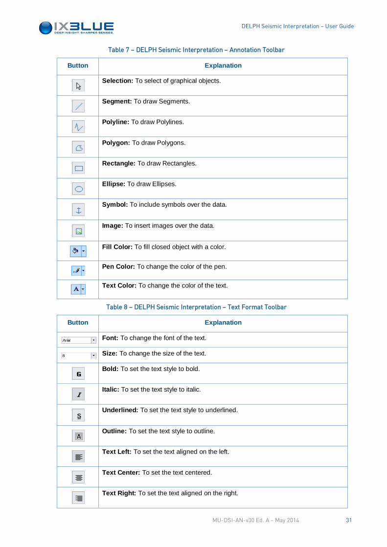
Table 7 – DELPH Seismic Interpretation – Annotation Toolbar
Button Explanation
Selection: To select of graphical objects.
Segment: To draw Segments.
Polyline: To draw Polylines.
Polygon: To draw Polygons.
Rectangle: To draw Rectangles.
Ellipse: To draw Ellipses.
Symbol: To include symbols over the data.
Image: To insert images over the data.
Fill Color: To fill closed object with a color.
Pen Color: To change the color of the pen.
Text Color: To change the color of the text.
Table 8 – DELPH Seismic Interpretation – Text Format Toolbar
Button Explanation
Font: To change the font of the text.
Size: To change the size of the text.
Bold: To set the text style to bold.
Italic: To set the text style to italic.
Underlined: To set the text style to underlined.
Outline: To set the text style to outline.
Text Left: To set the text aligned on the left.
Text Center: To set the text centered.
Text Right: To set the text aligned on the right.
MU-DSI-AN-v30 Ed. A – May 2014 31
DELPH Seismic Interpretation – User Guide
V.2.4 USING THE KEYPAD AND THE MOUSE
These hints are mainly designed to help the bottom digitalization.
Arrow Keys
• The arrow keys have the following functions
• Right arrow: it moves the profile horizontally towards the increasing distances
• Left arrow: it moves the profile horizontally towards the decreasing distances
• Up arrow: it moves the profile vertically towards the decreasing times
• Down arrow: it moves the profile vertically towards the increasing times
[Shift]: If you press the [Shift] key at the same time as the arrows scrolls the whole
page up and down.
[+] and [-] Keys
• [+] key is a shortcut key to zoom in
• [-] key is a shortcut key to zoom out
Page Up and Page Down Keys
• [Page Up] key is a shortcut key to scroll the image vertically towards the increasing
distances by 80% of the image size
• [Page Down] key is a shortcut key to scroll the image vertically towards the
decreasing distances by 80% of the image size
[F] Keys for Processing Launch
• [F5] key is a shortcut key to launch the processing
• [F6] key is a shortcut key to select the processing for the visible data or all data
Wheel Mouse
You can also use the wheel mouse button (if any) to move vertically the seismic profile.
• The [Del] key deletes the selected fragment
• The [Backspace] key deletes the rightmost point digitized
• The [Esc] key pauses the automatic tracking
• The [F9] key takes a print screen, snapshot tool
V.2.5 DISPLAYED UNITS
You can select the unit that the data is displayed in. You can display the
• Positions in the input or output geodesy, in the geographic or projected mode and in
various numeric formats
• Range in various distance units or traveled time with a specific precision
• Geographic Distance in various distance units with a specific precision
• Processing Distance in various distance units with a specific precision
• KP Kilometer Point with a specific precision
• Processing Travel Time in various distance units with a specific precision
• Travel Time in various time units with a specific precision
• Altitude / Depth in various distance units with a specific precision
MU-DSI-AN-v30 Ed. A – May 2014 32
DELPH Seismic Interpretation – User Guide
• Angle in degrees or radians with a specific precision
• Frequency in Hertz or Kilohertz with a specific precision
• Celerity in meter/second with a specific precision
• Speed in m/s, km/h and knots with a specific precision
See in Appendix 0 the conversion values between units.
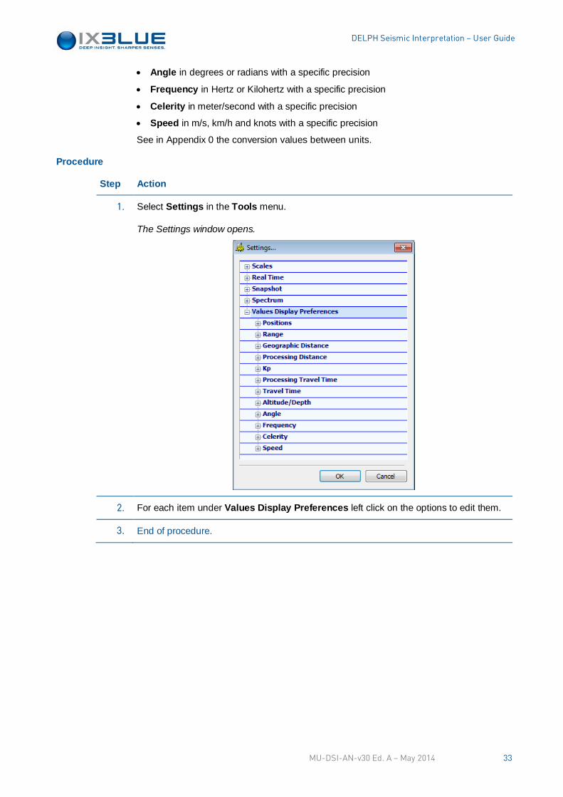
Procedure
Step Action
1. Select Settings in the Tools menu.
The Settings window opens.
2. For each item under Values Display Preferences left click on the options to edit them.
3. End of procedure.
MU-DSI-AN-v30 Ed. A – May 2014 33
DELPH Seismic Interpretation – User Guide
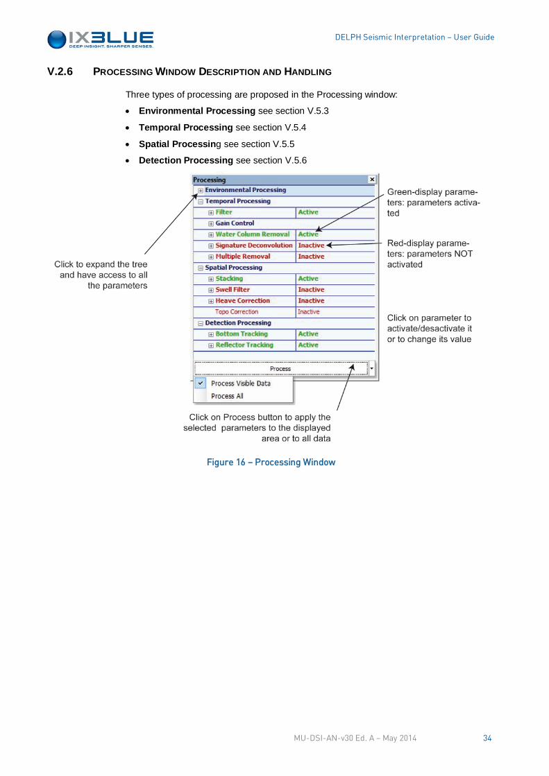
V.2.6 PROCESSING WINDOW DESCRIPTION AND HANDLING
Three types of processing are proposed in the Processing window:
• Environmental Processing see section V.5.3
• Temporal Processing see section V.5.4
• Spatial Processing see section V.5.5
• Detection Processing see section V.5.6
Figure 16 – Processing Window
MU-DSI-AN-v30 Ed. A – May 2014 34
DELPH Seismic Interpretation – User Guide
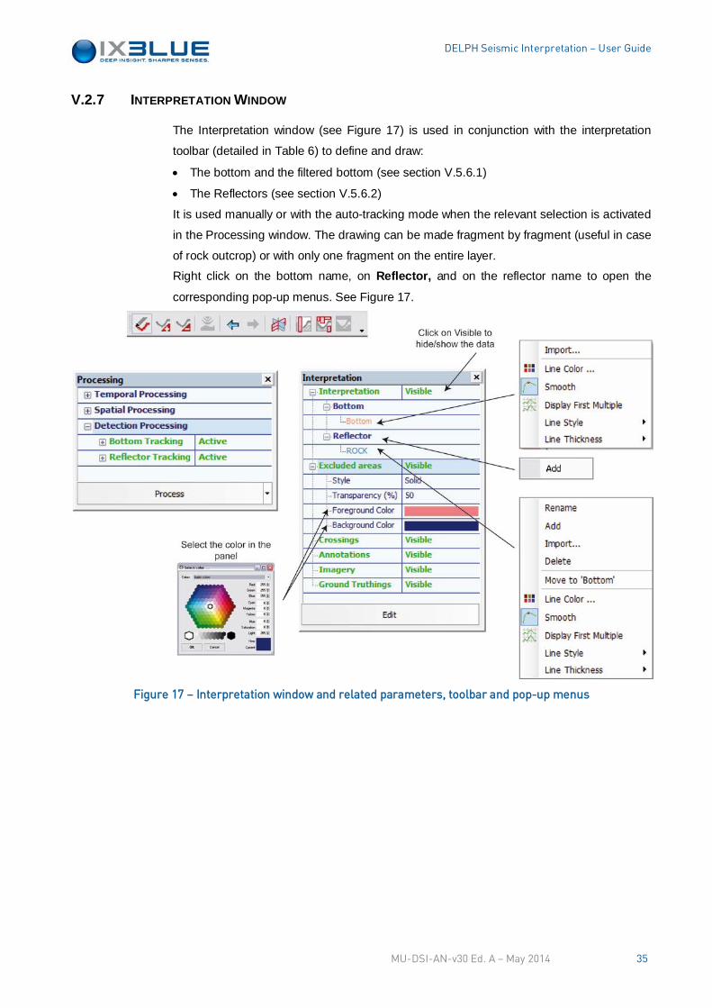
V.2.7 INTERPRETATION WINDOW
The Interpretation window (see Figure 17) is used in conjunction with the interpretation
toolbar (detailed in Table 6) to define and draw:
• The bottom and the filtered bottom (see section V.5.6.1)
• The Reflectors (see section V.5.6.2)
It is used manually or with the auto-tracking mode when the relevant selection is activated
in the Processing window. The drawing can be made fragment by fragment (useful in case
of rock outcrop) or with only one fragment on the entire layer.
Right click on the bottom name, on Reflector, and on the reflector name to open the
corresponding pop-up menus. See Figure 17.
Figure 17 – Interpretation window and related parameters, toolbar and pop-up menus
MU-DSI-AN-v30 Ed. A – May 2014 35
DELPH Seismic Interpretation – User Guide
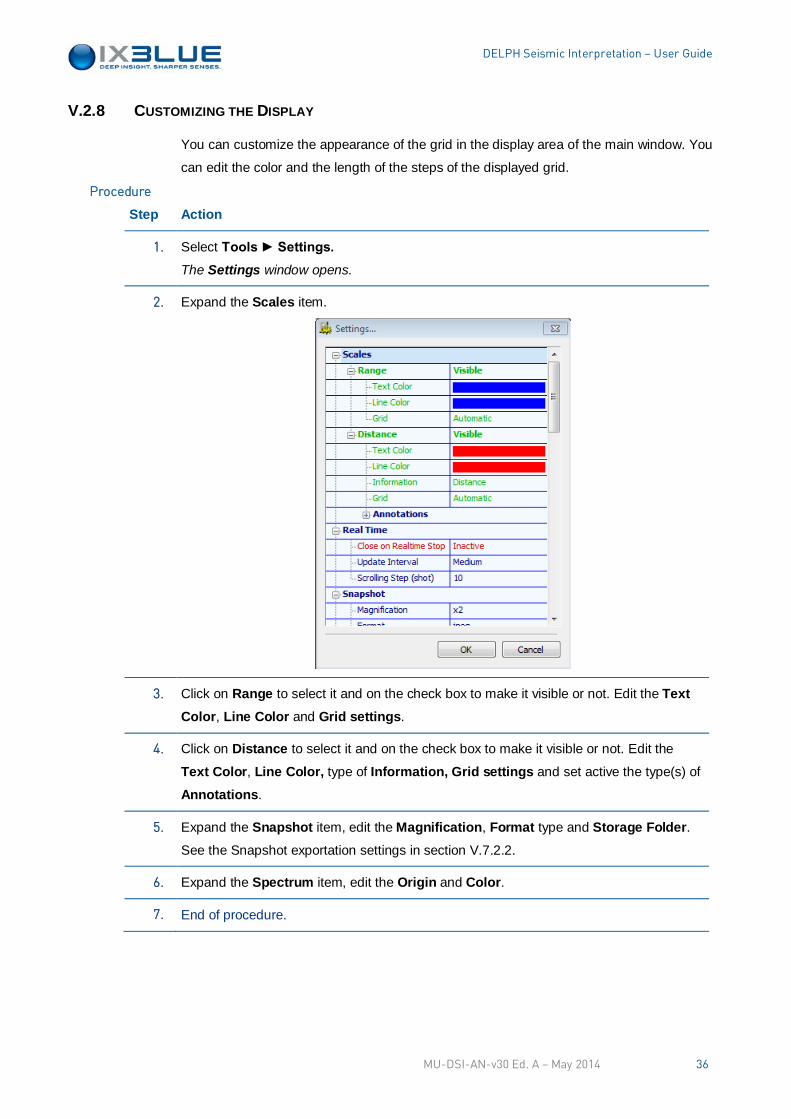
V.2.8 CUSTOMIZING THE DISPLAY
You can customize the appearance of the grid in the display area of the main window. You
can edit the color and the length of the steps of the displayed grid.
Step Action
1. Select Tools ► Settings. The Settings window opens.
2. Expand the Scales item.
3. Click on Range to select it and on the check box to make it visible or not. Edit the Text Color, Line Color and Grid settings.
4. Click on Distance to select it and on the check box to make it visible or not. Edit the
Text Color, Line Color, type of Information, Grid settings and set active the type(s) of
Annotations.
5. Expand the Snapshot item, edit the Magnification, Format type and Storage Folder. See the Snapshot exportation settings in section V.7.2.2.
6. Expand the Spectrum item, edit the Origin and Color.
7. End of procedure.
Procedure
MU-DSI-AN-v30 Ed. A – May 2014 36
DELPH Seismic Interpretation – User Guide
V.3 Correcting from the Layback and System Geometry
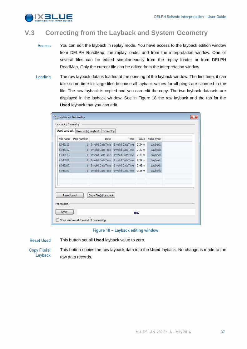
You can edit the layback in replay mode. You have access to the layback edition window
from DELPH RoadMap, the replay loader and from the interpretation window. One or
several files can be edited simultaneously from the replay loader or from DELPH
RoadMap. Only the current file can be edited from the interpretation window.
The raw layback data is loaded at the opening of the layback window. The first time, it can
take some time for large files because all layback values for all pings are scanned in the
file. The raw layback is copied and you can edit the copy. The two layback datasets are
displayed in the layback window. See in Figure 18 the raw layback and the tab for the
Used layback that you can edit.
Figure 18 – Layback editing window
This button set all Used layback value to zero.
This button copies the raw layback data into the Used layback. No change is made to the
raw data records.
Access
Loading
Reset Used
Copy File(s) Layback
MU-DSI-AN-v30 Ed. A – May 2014 37
DELPH Seismic Interpretation – User Guide
V.3.1 EDITING THE LAYBACK
Adding a Layback
Step Action
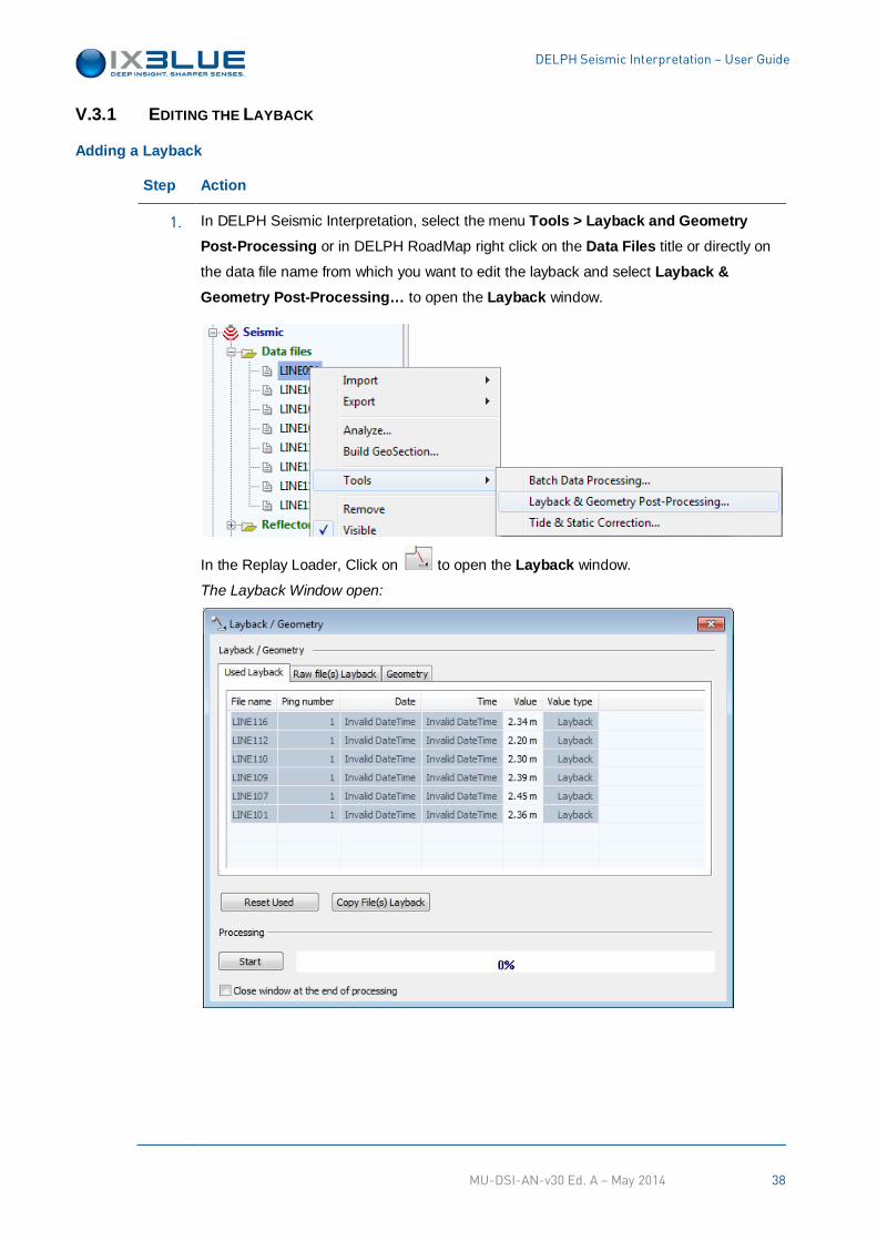
1. In DELPH Seismic Interpretation, select the menu Tools > Layback and Geometry Post-Processing or in DELPH RoadMap right click on the Data Files title or directly on
the data file name from which you want to edit the layback and select Layback & Geometry Post-Processing… to open the Layback window.
In the Replay Loader, Click on to open the Layback window.
The Layback Window open:
MU-DSI-AN-v30 Ed. A – May 2014 38
DELPH Seismic Interpretation – User Guide
Step Action
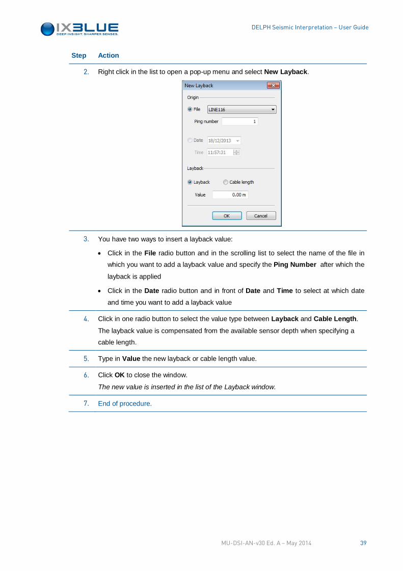
2. Right click in the list to open a pop-up menu and select New Layback.
3. You have two ways to insert a layback value:
• Click in the File radio button and in the scrolling list to select the name of the file in
which you want to add a layback value and specify the Ping Number after which the
layback is applied
• Click in the Date radio button and in front of Date and Time to select at which date
and time you want to add a layback value
4. Click in one radio button to select the value type between Layback and Cable Length.
The layback value is compensated from the available sensor depth when specifying a
cable length.
5. Type in Value the new layback or cable length value.
6. Click OK to close the window.
The new value is inserted in the list of the Layback window.
7. End of procedure.
MU-DSI-AN-v30 Ed. A – May 2014 39
DELPH Seismic Interpretation – User Guide
Removing a Layback
Step Action
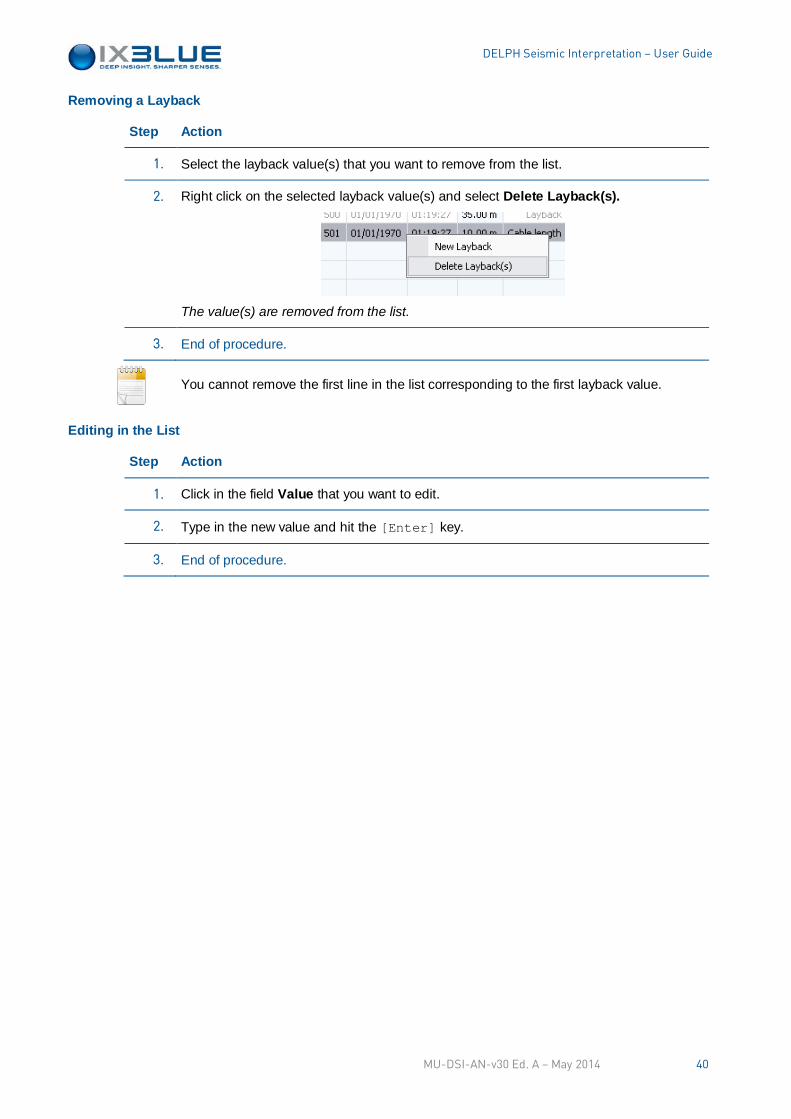
1. Select the layback value(s) that you want to remove from the list.
2. Right click on the selected layback value(s) and select Delete Layback(s).
The value(s) are removed from the list.
3. End of procedure.
You cannot remove the first line in the list corresponding to the first layback value.
Editing in the List
Step Action
1. Click in the field Value that you want to edit.
2. Type in the new value and hit the [Enter] key.
3. End of procedure.
MU-DSI-AN-v30 Ed. A – May 2014 40
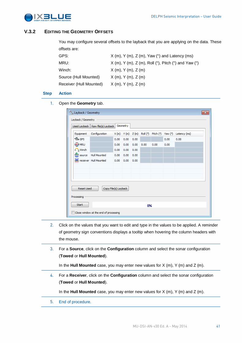
DELPH Seismic Interpretation – User Guide
V.3.2 EDITING THE GEOMETRY OFFSETS
You may configure several offsets to the layback that you are applying on the data. These
offsets are:
GPS: X (m), Y (m), Z (m), Yaw (°) and Latency (ms)
MRU: X (m), Y (m), Z (m), Roll (°), Pitch (°) and Yaw (°)
Winch: X (m), Y (m), Z (m)
Source (Hull Mounted) X (m), Y (m), Z (m)
Receiver (Hull Mounted) X (m), Y (m), Z (m)
Step Action
1. Open the Geometry tab.
2. Click on the values that you want to edit and type in the values to be applied. A reminder
of geometry sign conventions displays a tooltip when hovering the column headers with
the mouse.
3. For a Source, click on the Configuration column and select the sonar configuration
(Towed or Hull Mounted).
In the Hull Mounted case, you may enter new values for X (m), Y (m) and Z (m).
4. For a Receiver, click on the Configuration column and select the sonar configuration
(Towed or Hull Mounted).
In the Hull Mounted case, you may enter new values for X (m), Y (m) and Z (m).
5. End of procedure.
MU-DSI-AN-v30 Ed. A – May 2014 41
DELPH Seismic Interpretation – User Guide
V.3.3 STARTING THE PROCESS
Step Action
1. Click on the bottom check box if you want the window to be closed at the end of the
processing.
2. Once you have edited the layback, you can apply it to the current file(s). Click on Start.
The progress bar shows the processing status. The Start button is changed in a Stop
button.
3. You can stop the process at any time by clicking on the Stop button.
You are warned that interrupting the process can corrupt the file navigation.
4. End of procedure.
Procedure
MU-DSI-AN-v30 Ed. A – May 2014 42
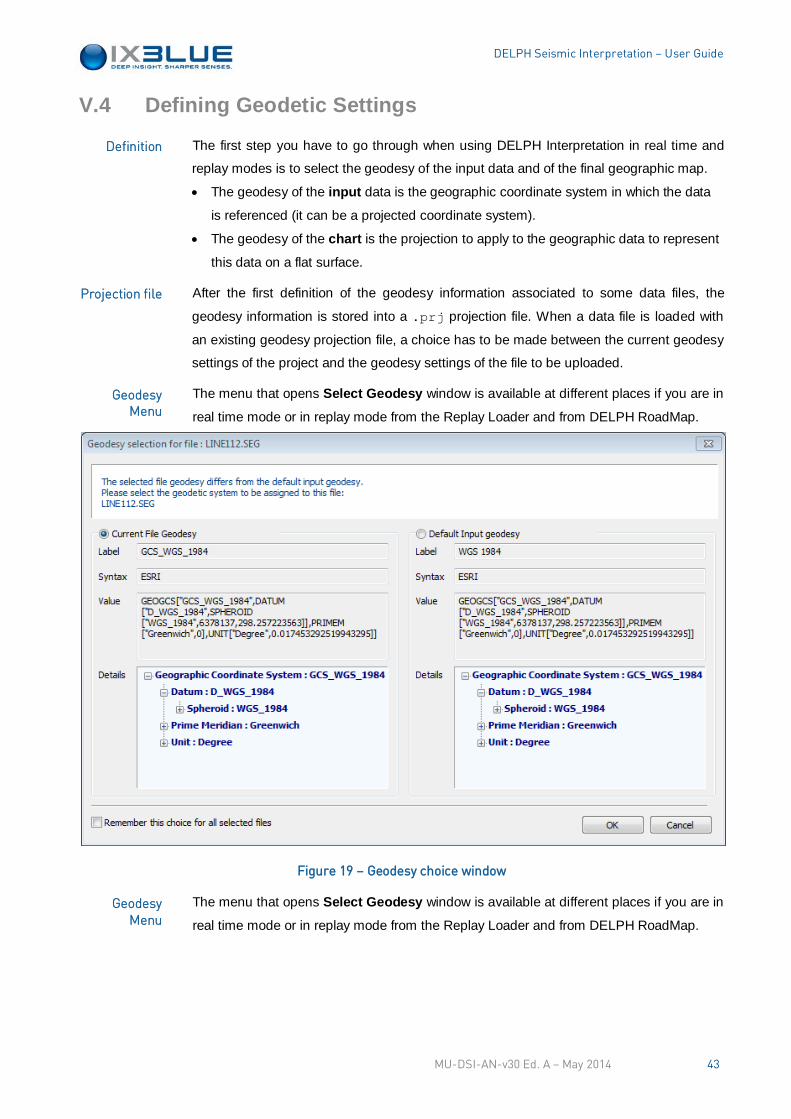
DELPH Seismic Interpretation – User Guide
V.4 Defining Geodetic Settings
The first step you have to go through when using DELPH Interpretation in real time and
replay modes is to select the geodesy of the input data and of the final geographic map.
• The geodesy of the input data is the geographic coordinate system in which the data
is referenced (it can be a projected coordinate system).
• The geodesy of the chart is the projection to apply to the geographic data to represent
this data on a flat surface.
After the first definition of the geodesy information associated to some data files, the
geodesy information is stored into a .prj projection file. When a data file is loaded with
an existing geodesy projection file, a choice has to be made between the current geodesy
settings of the project and the geodesy settings of the file to be uploaded.
The menu that opens Select Geodesy window is available at different places if you are in
real time mode or in replay mode from the Replay Loader and from DELPH RoadMap.
Figure 19 – Geodesy choice window
The menu that opens Select Geodesy window is available at different places if you are in
real time mode or in replay mode from the Replay Loader and from DELPH RoadMap.
Definition
Projection file
Geodesy Menu
Geodesy Menu
MU-DSI-AN-v30 Ed. A – May 2014 43
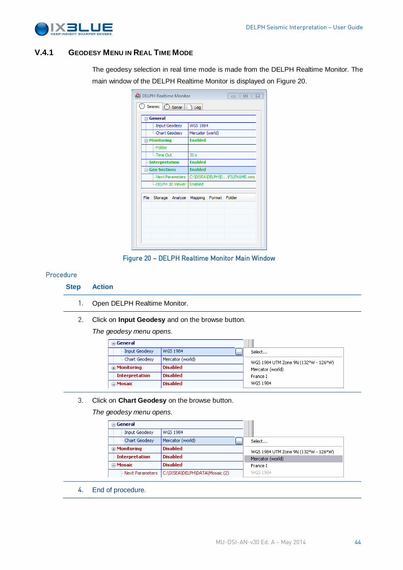
DELPH Seismic Interpretation – User Guide
V.4.1 GEODESY MENU IN REAL TIME MODE
The geodesy selection in real time mode is made from the DELPH Realtime Monitor. The
main window of the DELPH Realtime Monitor is displayed on Figure 20.
Figure 20 – DELPH Realtime Monitor Main Window
Step Action
1. Open DELPH Realtime Monitor.
2. Click on Input Geodesy and on the browse button.
The geodesy menu opens.
3. Click on Chart Geodesy on the browse button.
The geodesy menu opens.
4. End of procedure.
Procedure
MU-DSI-AN-v30 Ed. A – May 2014 44
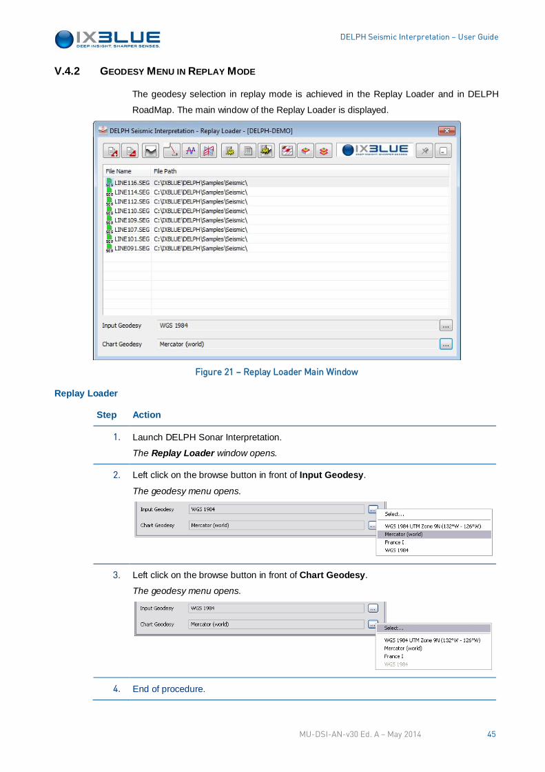
DELPH Seismic Interpretation – User Guide
V.4.2 GEODESY MENU IN REPLAY MODE
The geodesy selection in replay mode is achieved in the Replay Loader and in DELPH
RoadMap. The main window of the Replay Loader is displayed.
Figure 21 – Replay Loader Main Window
Replay Loader
Step Action
1. Launch DELPH Sonar Interpretation.
The Replay Loader window opens.
2. Left click on the browse button in front of Input Geodesy.
The geodesy menu opens.
3. Left click on the browse button in front of Chart Geodesy.
The geodesy menu opens.
4. End of procedure.
MU-DSI-AN-v30 Ed. A – May 2014 45
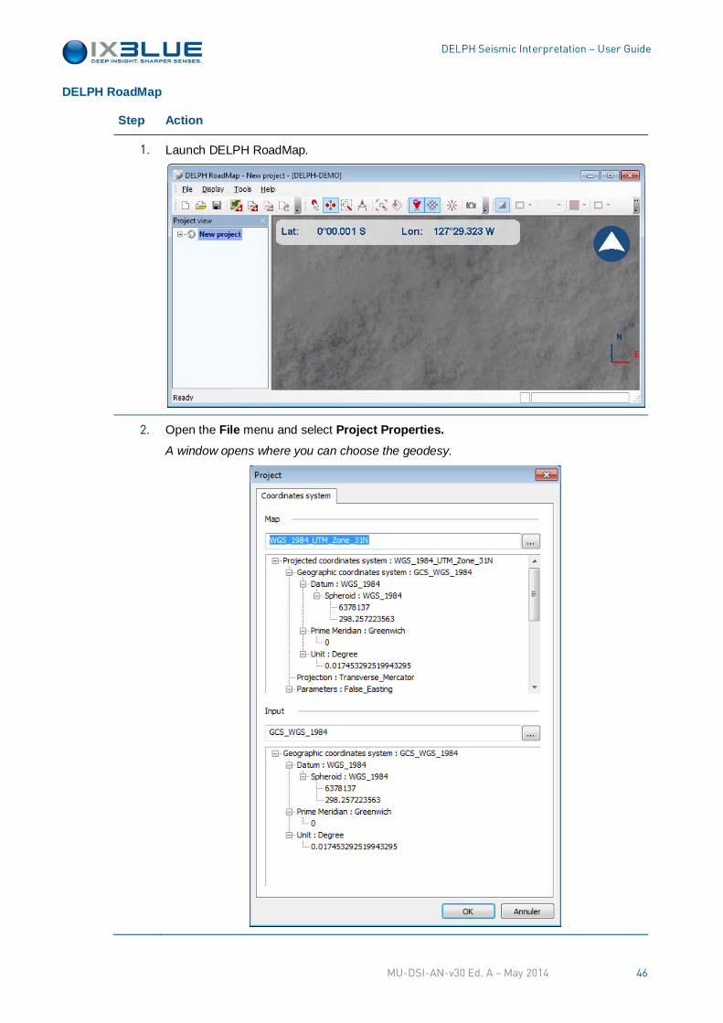
DELPH Seismic Interpretation – User Guide
DELPH RoadMap
Step Action
1. Launch DELPH RoadMap.
2. Open the File menu and select Project Properties. A window opens where you can choose the geodesy.
MU-DSI-AN-v30 Ed. A – May 2014 46
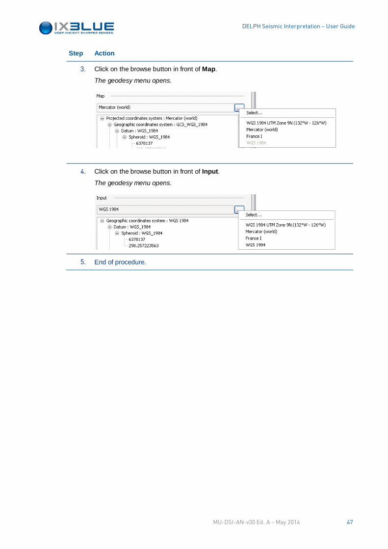
DELPH Seismic Interpretation – User Guide
Step Action
3. Click on the browse button in front of Map.
The geodesy menu opens.
4. Click on the browse button in front of Input.
The geodesy menu opens.
5. End of procedure.
MU-DSI-AN-v30 Ed. A – May 2014 47
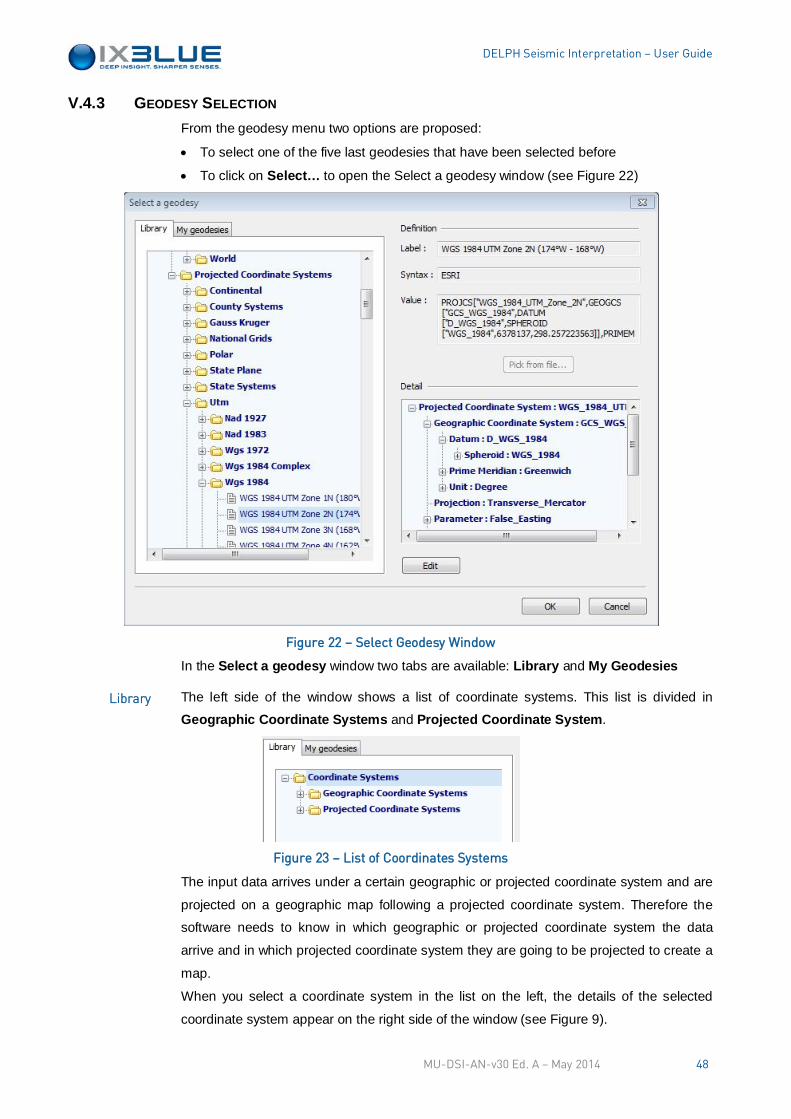
DELPH Seismic Interpretation – User Guide
V.4.3 GEODESY SELECTION From the geodesy menu two options are proposed:
• To select one of the five last geodesies that have been selected before
• To click on Select… to open the Select a geodesy window (see Figure 22)
Figure 22 – Select Geodesy Window
In the Select a geodesy window two tabs are available: Library and My Geodesies
The left side of the window shows a list of coordinate systems. This list is divided in
Geographic Coordinate Systems and Projected Coordinate System.
Figure 23 – List of Coordinates Systems
The input data arrives under a certain geographic or projected coordinate system and are
projected on a geographic map following a projected coordinate system. Therefore the
software needs to know in which geographic or projected coordinate system the data
arrive and in which projected coordinate system they are going to be projected to create a
map.
When you select a coordinate system in the list on the left, the details of the selected
coordinate system appear on the right side of the window (see Figure 9).
Library
MU-DSI-AN-v30 Ed. A – May 2014 48
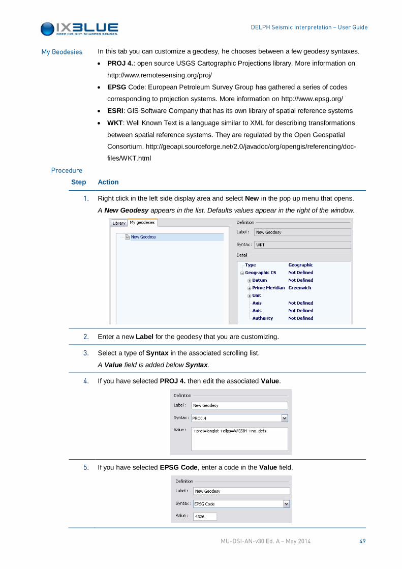
DELPH Seismic Interpretation – User Guide
In this tab you can customize a geodesy, he chooses between a few geodesy syntaxes.
• PROJ 4.: open source USGS Cartographic Projections library. More information on
http://www.remotesensing.org/proj/
• EPSG Code: European Petroleum Survey Group has gathered a series of codes
corresponding to projection systems. More information on http://www.epsg.org/
• ESRI: GIS Software Company that has its own library of spatial reference systems
• WKT: Well Known Text is a language similar to XML for describing transformations
between spatial reference systems. They are regulated by the Open Geospatial
Consortium. http://geoapi.sourceforge.net/2.0/javadoc/org/opengis/referencing/doc-
files/WKT.html
Step Action
1. Right click in the left side display area and select New in the pop up menu that opens.
A New Geodesy appears in the list. Defaults values appear in the right of the window.
2. Enter a new Label for the geodesy that you are customizing.
3. Select a type of Syntax in the associated scrolling list.
A Value field is added below Syntax.
4. If you have selected PROJ 4. then edit the associated Value.
5. If you have selected EPSG Code, enter a code in the Value field.
My Geodesies
Procedure
MU-DSI-AN-v30 Ed. A – May 2014 49
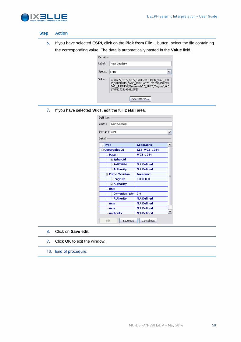
DELPH Seismic Interpretation – User Guide
Step Action
6. If you have selected ESRI, click on the Pick from File… button, select the file containing
the corresponding value. The data is automatically pasted in the Value field.
7. If you have selected WKT, edit the full Detail area.
8. Click on Save edit.
9. Click OK to exit the window.
10. End of procedure.
MU-DSI-AN-v30 Ed. A – May 2014 50
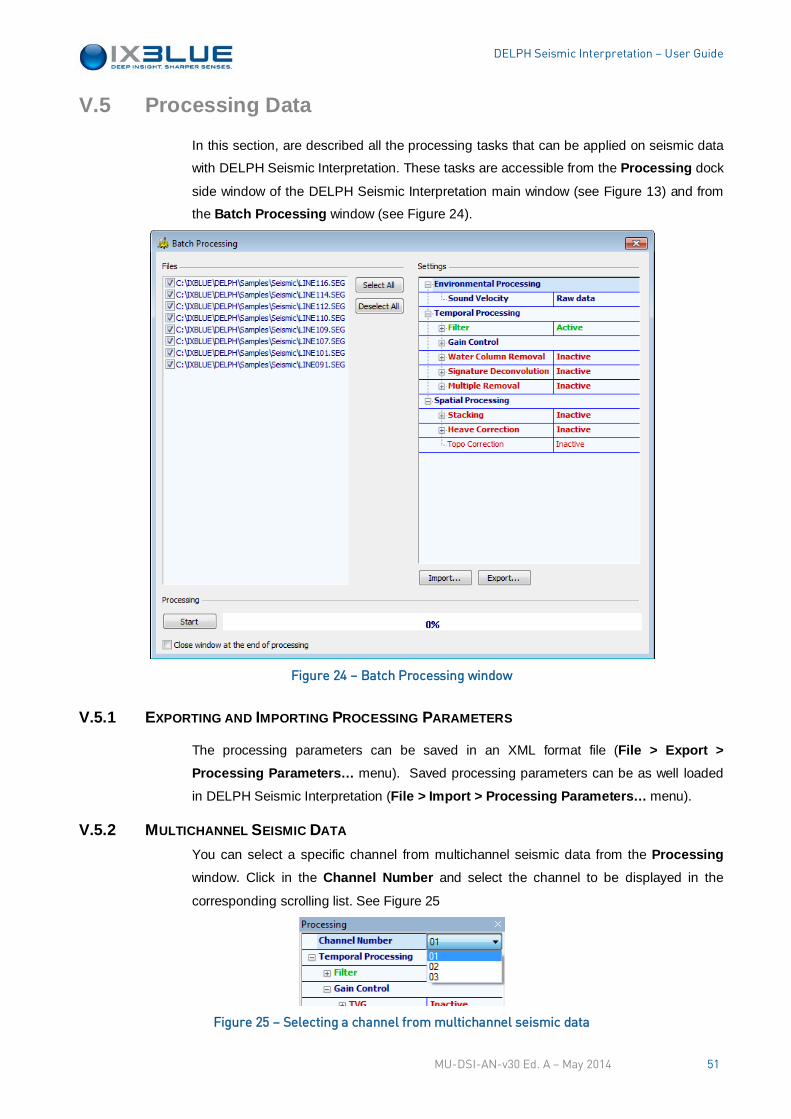
DELPH Seismic Interpretation – User Guide
V.5 Processing Data
In this section, are described all the processing tasks that can be applied on seismic data
with DELPH Seismic Interpretation. These tasks are accessible from the Processing dock
side window of the DELPH Seismic Interpretation main window (see Figure 13) and from
the Batch Processing window (see Figure 24).
Figure 24 – Batch Processing window
V.5.1 EXPORTING AND IMPORTING PROCESSING PARAMETERS
The processing parameters can be saved in an XML format file (File > Export > Processing Parameters… menu). Saved processing parameters can be as well loaded
in DELPH Seismic Interpretation (File > Import > Processing Parameters… menu).
V.5.2 MULTICHANNEL SEISMIC DATA You can select a specific channel from multichannel seismic data from the Processing
window. Click in the Channel Number and select the channel to be displayed in the
corresponding scrolling list. See Figure 25
Figure 25 – Selecting a channel from multichannel seismic data
MU-DSI-AN-v30 Ed. A – May 2014 51
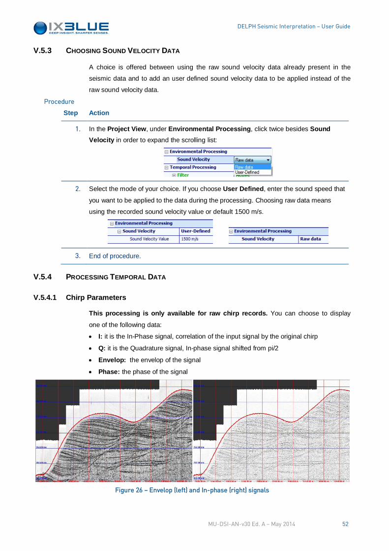
DELPH Seismic Interpretation – User Guide
V.5.3 CHOOSING SOUND VELOCITY DATA
A choice is offered between using the raw sound velocity data already present in the
seismic data and to add an user defined sound velocity data to be applied instead of the
raw sound velocity data.
Step Action
1. In the Project View, under Environmental Processing, click twice besides Sound Velocity in order to expand the scrolling list:
2. Select the mode of your choice. If you choose User Defined, enter the sound speed that
you want to be applied to the data during the processing. Choosing raw data means
using the recorded sound velocity value or default 1500 m/s.
3. End of procedure.
V.5.4 PROCESSING TEMPORAL DATA
V.5.4.1 Chirp Parameters
This processing is only available for raw chirp records. You can choose to display
one of the following data:
• I: it is the In-Phase signal, correlation of the input signal by the original chirp
• Q: it is the Quadrature signal, In-phase signal shifted from pi/2
• Envelop: the envelop of the signal
• Phase: the phase of the signal
Figure 26 – Envelop (left) and In-phase (right) signals
Procedure
MU-DSI-AN-v30 Ed. A – May 2014 52
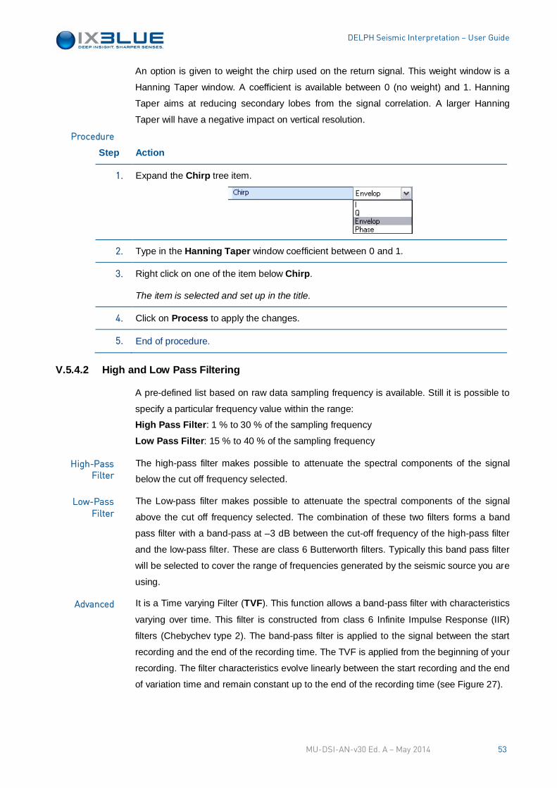
DELPH Seismic Interpretation – User Guide
An option is given to weight the chirp used on the return signal. This weight window is a
Hanning Taper window. A coefficient is available between 0 (no weight) and 1. Hanning
Taper aims at reducing secondary lobes from the signal correlation. A larger Hanning
Taper will have a negative impact on vertical resolution.
Step Action
1. Expand the Chirp tree item.
2. Type in the Hanning Taper window coefficient between 0 and 1.
3. Right click on one of the item below Chirp.
The item is selected and set up in the title.
4. Click on Process to apply the changes.
5. End of procedure.
V.5.4.2 High and Low Pass Filtering
A pre-defined list based on raw data sampling frequency is available. Still it is possible to
specify a particular frequency value within the range:
High Pass Filter: 1 % to 30 % of the sampling frequency
Low Pass Filter: 15 % to 40 % of the sampling frequency
The high-pass filter makes possible to attenuate the spectral components of the signal
below the cut off frequency selected.
The Low-pass filter makes possible to attenuate the spectral components of the signal
above the cut off frequency selected. The combination of these two filters forms a band
pass filter with a band-pass at –3 dB between the cut-off frequency of the high-pass filter
and the low-pass filter. These are class 6 Butterworth filters. Typically this band pass filter
will be selected to cover the range of frequencies generated by the seismic source you are
using.
It is a Time varying Filter (TVF). This function allows a band-pass filter with characteristics
varying over time. This filter is constructed from class 6 Infinite Impulse Response (IIR)
filters (Chebychev type 2). The band-pass filter is applied to the signal between the start
recording and the end of the recording time. The TVF is applied from the beginning of your
recording. The filter characteristics evolve linearly between the start recording and the end
of variation time and remain constant up to the end of the recording time (see Figure 27).
Procedure
High-Pass Filter
Low-Pass Filter
Advanced
MU-DSI-AN-v30 Ed. A – May 2014 53
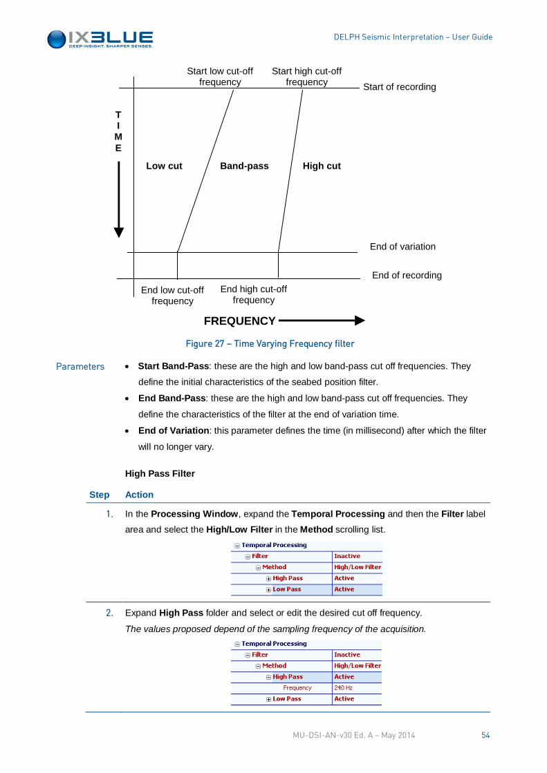
DELPH Seismic Interpretation – User Guide
T I ME
FREQUENCY
Start of recording
End of variation
End of recording
Start low cut-off frequency
Start high cut-off frequency
End low cut-off frequency
End high cut-off frequency
Low cut High cut Band-pass
Figure 27 – Time Varying Frequency filter
• Start Band-Pass: these are the high and low band-pass cut off frequencies. They
define the initial characteristics of the seabed position filter.
• End Band-Pass: these are the high and low band-pass cut off frequencies. They
define the characteristics of the filter at the end of variation time.
• End of Variation: this parameter defines the time (in millisecond) after which the filter
will no longer vary.
High Pass Filter
Step Action
1. In the Processing Window, expand the Temporal Processing and then the Filter label area and select the High/Low Filter in the Method scrolling list.
2. Expand High Pass folder and select or edit the desired cut off frequency.
The values proposed depend of the sampling frequency of the acquisition.
Parameters
MU-DSI-AN-v30 Ed. A – May 2014 54
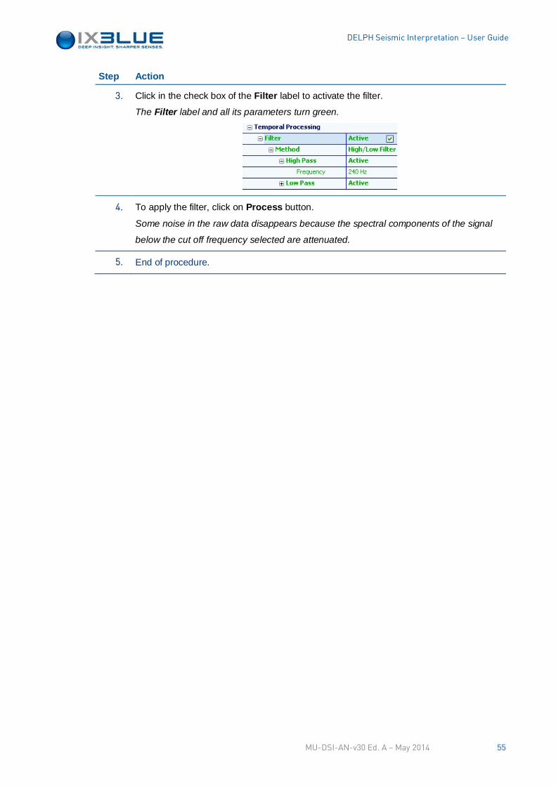
DELPH Seismic Interpretation – User Guide
Step Action
3. Click in the check box of the Filter label to activate the filter.
The Filter label and all its parameters turn green.
4. To apply the filter, click on Process button.
Some noise in the raw data disappears because the spectral components of the signal
below the cut off frequency selected are attenuated.
5. End of procedure.
MU-DSI-AN-v30 Ed. A – May 2014 55
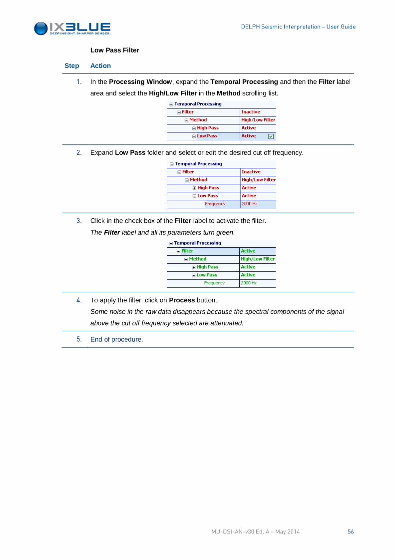
DELPH Seismic Interpretation – User Guide
Low Pass Filter
Step Action
1. In the Processing Window, expand the Temporal Processing and then the Filter label area and select the High/Low Filter in the Method scrolling list.
2. Expand Low Pass folder and select or edit the desired cut off frequency.
3. Click in the check box of the Filter label to activate the filter.
The Filter label and all its parameters turn green.
4. To apply the filter, click on Process button.
Some noise in the raw data disappears because the spectral components of the signal
above the cut off frequency selected are attenuated.
5. End of procedure.
MU-DSI-AN-v30 Ed. A – May 2014 56
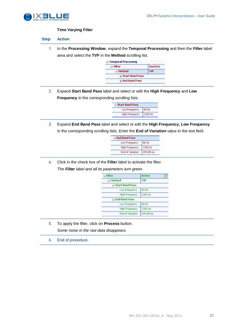
DELPH Seismic Interpretation – User Guide
Time Varying Filter
Step Action
1. In the Processing Window, expand the Temporal Processing and then the Filter label area and select the TVF in the Method scrolling list.
2. Expand Start Band Pass label and select or edit the High Frequency and Low Frequency in the corresponding scrolling lists.
3. Expand End Band Pass label and select or edit the High Frequency, Low Frequency
in the corresponding scrolling lists. Enter the End of Variation value in the text field.
4. Click in the check box of the Filter label to activate the filter.
The Filter label and all its parameters turn green.
5. To apply the filter, click on Process button.
Some noise in the raw data disappears.
6. End of procedure.
MU-DSI-AN-v30 Ed. A – May 2014 57
DELPH Seismic Interpretation – User Guide
V.5.4.3 Gain Control
This option offers improved visualization of the seismic signals. The principle is to
compensate the variations in the signal envelope by different functions:
• Time Varying Gain (TVG)
• Automatic Gain Control (AGC) decremental
• AGC linear
• AGC exponential
• AGC Power
With the AGC the data within a specified time window is gained to a constant energy level.
The window is slid down the trace so the energy is equilibrated. Shorter windows boost
everything while longer windows tend to show true relative amplitudes.
AGC and TVG variants both employ a fixed window length. The trace is divided into
consecutive windows of equal length (a trace consists of the samples collected during one
shot). The envelope is the set of maximum values found for each window.
The window length determines the increment for envelope sampling, and subsequently
the gain correction function. It is assumed that this function will not vary significantly over
a time period shorter than that of the source signature (at the risk of introducing major
distortion of the signal), and it is not advisable to select a window the length of which is
less than the signature length.
The AGCs have a signal-dependent gain correction curve. This signal-dependent gain
correction curve contrasts with the time-variable gain for which the gain correction curve is
exclusively time-dependent.
This function applies a gain correction curve that varies linearly as a function of time between the Start Gain and the End Gain of the trace.
This type of AGC is designed to conserve quantitative information on the relative power of
the reflectors while limiting the signal dynamics. It is assumed that the signal amplitude is
strictly decreasing over time. If the condition is not respected, the processing will not give
correct results.
This form is determined as follows: A secondary envelope is calculated by interpolation
between the extremes of the initial signal envelope, while limiting the search for each
extreme to a range between the preceding extreme and the end of the trace. The
correction curve is inversely proportional to this secondary envelope.
Parameter:
Window: it is the window length used to calculate the signal envelope.
This gain method does not yield good results in the presence of multiple echoes of the sea
floor, or of a surface echo generated by deep sources such as “Deep tow”. The
assumption of increasing signal attenuation over time is not valid for those cases.
Gain Control Principles
TVG Parameters
AGC Decremental
MU-DSI-AN-v30 Ed. A – May 2014 58
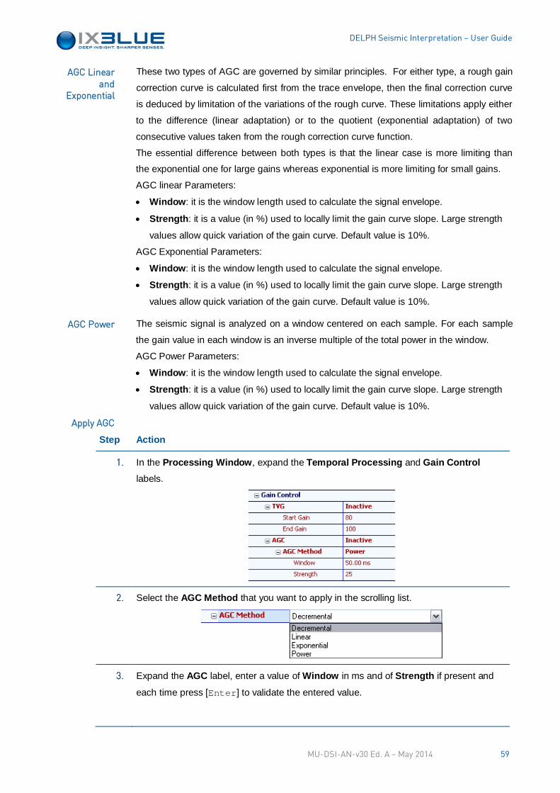
DELPH Seismic Interpretation – User Guide
These two types of AGC are governed by similar principles. For either type, a rough gain
correction curve is calculated first from the trace envelope, then the final correction curve
is deduced by limitation of the variations of the rough curve. These limitations apply either
to the difference (linear adaptation) or to the quotient (exponential adaptation) of two
consecutive values taken from the rough correction curve function.
The essential difference between both types is that the linear case is more limiting than
the exponential one for large gains whereas exponential is more limiting for small gains.
AGC linear Parameters:
• Window: it is the window length used to calculate the signal envelope.
• Strength: it is a value (in %) used to locally limit the gain curve slope. Large strength
values allow quick variation of the gain curve. Default value is 10%.
AGC Exponential Parameters:
• Window: it is the window length used to calculate the signal envelope.
• Strength: it is a value (in %) used to locally limit the gain curve slope. Large strength
values allow quick variation of the gain curve. Default value is 10%.
The seismic signal is analyzed on a window centered on each sample. For each sample
the gain value in each window is an inverse multiple of the total power in the window.
AGC Power Parameters:
• Window: it is the window length used to calculate the signal envelope.
• Strength: it is a value (in %) used to locally limit the gain curve slope. Large strength
values allow quick variation of the gain curve. Default value is 10%.
Step Action
1. In the Processing Window, expand the Temporal Processing and Gain Control labels.
2. Select the AGC Method that you want to apply in the scrolling list.
3. Expand the AGC label, enter a value of Window in ms and of Strength if present and
each time press [Enter] to validate the entered value.
AGC Linear and
Exponential
AGC Power
Apply AGC
MU-DSI-AN-v30 Ed. A – May 2014 59
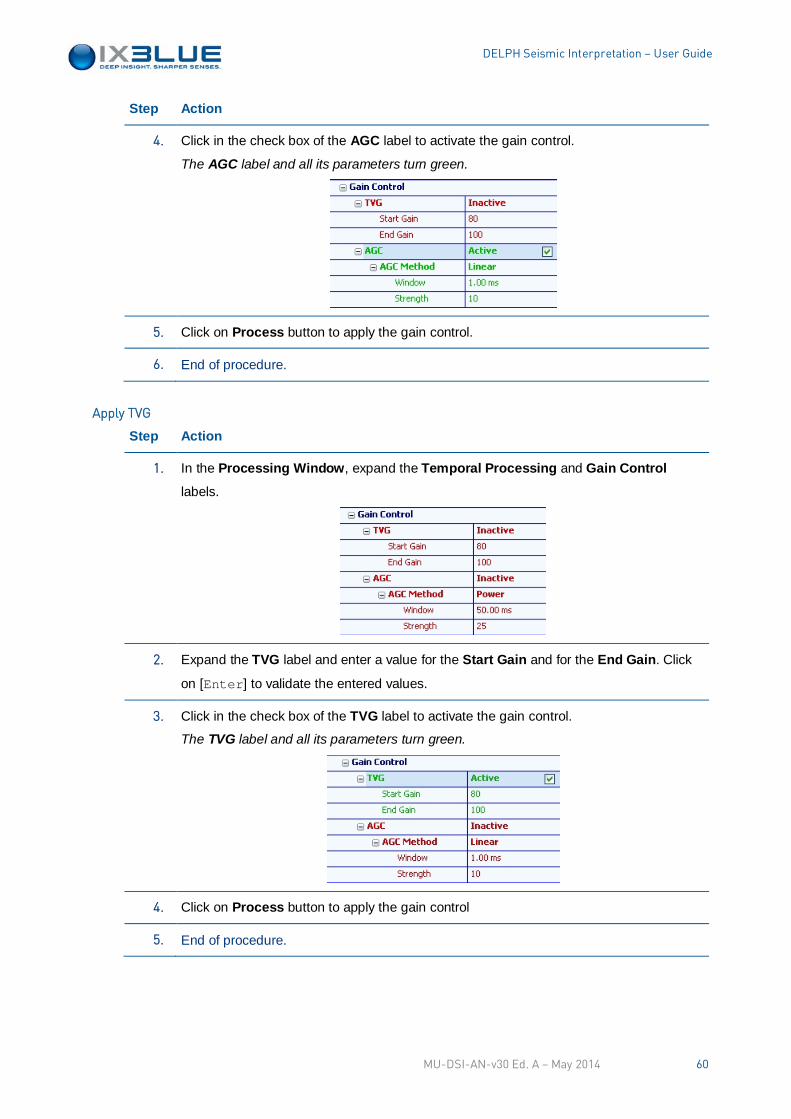
DELPH Seismic Interpretation – User Guide
Step Action
4. Click in the check box of the AGC label to activate the gain control.
The AGC label and all its parameters turn green.
5. Click on Process button to apply the gain control.
6. End of procedure.
Step Action
1. In the Processing Window, expand the Temporal Processing and Gain Control
labels.
2. Expand the TVG label and enter a value for the Start Gain and for the End Gain. Click
on [Enter] to validate the entered values.
3. Click in the check box of the TVG label to activate the gain control.
The TVG label and all its parameters turn green.
4. Click on Process button to apply the gain control
5. End of procedure.
Apply TVG
MU-DSI-AN-v30 Ed. A – May 2014 60
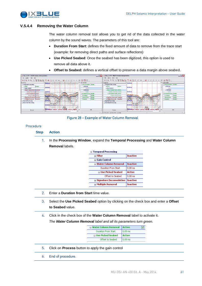
DELPH Seismic Interpretation – User Guide
V.5.4.4 Removing the Water Column
The water column removal tool allows you to get rid of the data collected in the water
column by the sound waves. The parameters of this tool are:
• Duration From Start: defines the fixed amount of data to remove from the trace start
(example: for removing direct paths and surface reflections)
• Use Picked Seabed: Once the seabed has been digitized, this option is used to
remove all data above it.
• Offset to Seabed: defines a vertical offset to preserve a data margin above seabed.
Figure 28 – Example of Water Column Removal
Step Action
1. In the Processing Window, expand the Temporal Processing and Water Column Removal labels.
2. Enter a Duration from Start time value.
3. Select the Use Picked Seabed option by clicking on the check box and enter a Offset to Seabed value.
4. Click in the check box of the Water Column Removal label to activate it.
The Water Column Removal label and all its parameters turn green.
5. Click on Process button to apply the gain control
6. End of procedure.
Procedure
MU-DSI-AN-v30 Ed. A – May 2014 61
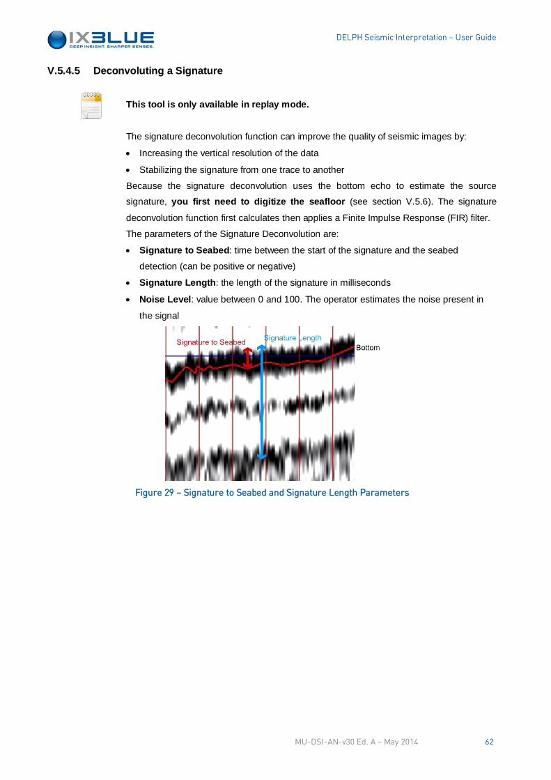
DELPH Seismic Interpretation – User Guide
V.5.4.5 Deconvoluting a Signature
This tool is only available in replay mode.
The signature deconvolution function can improve the quality of seismic images by:
• Increasing the vertical resolution of the data
• Stabilizing the signature from one trace to another
Because the signature deconvolution uses the bottom echo to estimate the source
signature, you first need to digitize the seafloor (see section V.5.6). The signature
deconvolution function first calculates then applies a Finite Impulse Response (FIR) filter.
The parameters of the Signature Deconvolution are:
• Signature to Seabed: time between the start of the signature and the seabed
detection (can be positive or negative)
• Signature Length: the length of the signature in milliseconds
• Noise Level: value between 0 and 100. The operator estimates the noise present in
the signal
Figure 29 – Signature to Seabed and Signature Length Parameters
MU-DSI-AN-v30 Ed. A – May 2014 62
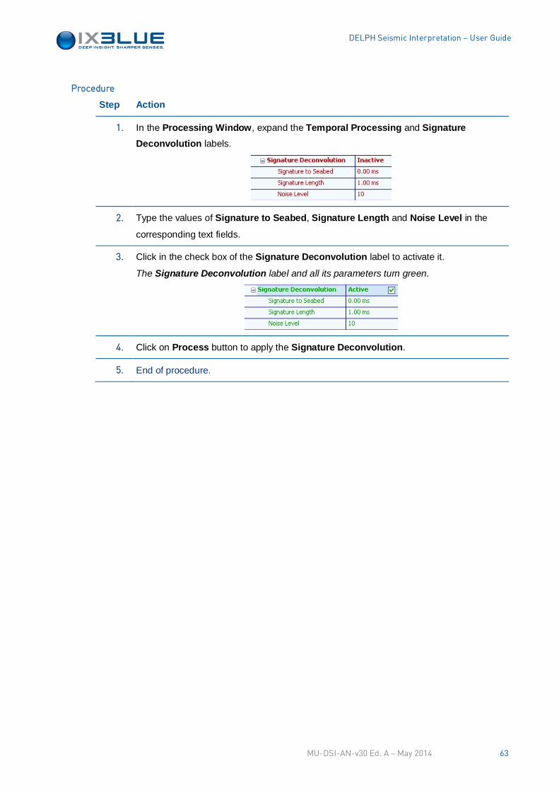
DELPH Seismic Interpretation – User Guide
Step Action
1. In the Processing Window, expand the Temporal Processing and Signature Deconvolution labels.
2. Type the values of Signature to Seabed, Signature Length and Noise Level in the
corresponding text fields.
3. Click in the check box of the Signature Deconvolution label to activate it.
The Signature Deconvolution label and all its parameters turn green.
4. Click on Process button to apply the Signature Deconvolution.
5. End of procedure.
Procedure
MU-DSI-AN-v30 Ed. A – May 2014 63
DELPH Seismic Interpretation – User Guide
V.5.4.6 Removing Multiple
This tool is only available in replay mode.
This function attenuates multiple echoes from the seabed. See Figure 29. This is called
predictive deconvolution. It requires the digitalization of the bottom (see section V.6).
The attenuation of seabed multiple is obtained by subtracting from digitized signal the
multiples predicted by using a predictive deconvolution algorithm. This processing
capability is applied independently to each trace and involves only seabed multiples
(multiples due to internal reflection are not processed).
• Signature to Seabed: beginning time of the seabed signature.
• Signature Length: the length of the signature in milliseconds. This parameter can be
easily measured in the Profile area. The signature length depends upon the seismic
source being used.
• Search Window: is the length in milliseconds of the processing window. This
parameter must be determined by successive approximations during processing. The
initial value entered allows only a rough setting that must be fine-tuned. This parameter
depends on filtering characteristics and on the geological structure of the terrain. Its
value must be situated between three sampling periods and half of the recording
length. The default value is equal to the minimum value.
• Filter Order: it defines the number of filter coefficients. The higher this number is, the
stronger the deconvolution. The values are limited to the [3,9] interval. The default is 3.
In practice, the minimum value is generally satisfactory, but if your data exhibits a very
low signal-to-noise ratio, it may be useful to increase this value (the calculation time is
then longer).
Parameters
MU-DSI-AN-v30 Ed. A – May 2014 64
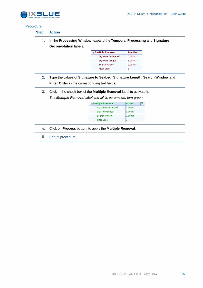
DELPH Seismic Interpretation – User Guide
Step Action
1. In the Processing Window, expand the Temporal Processing and Signature Deconvolution labels.
2. Type the values of Signature to Seabed, Signature Length, Search Window and
Filter Order in the corresponding text fields.
3. Click in the check box of the Multiple Removal label to activate it.
The Multiple Removal label and all its parameters turn green.
4. Click on Process button, to apply the Multiple Removal.
5. End of procedure.
Procedure
MU-DSI-AN-v30 Ed. A – May 2014 65
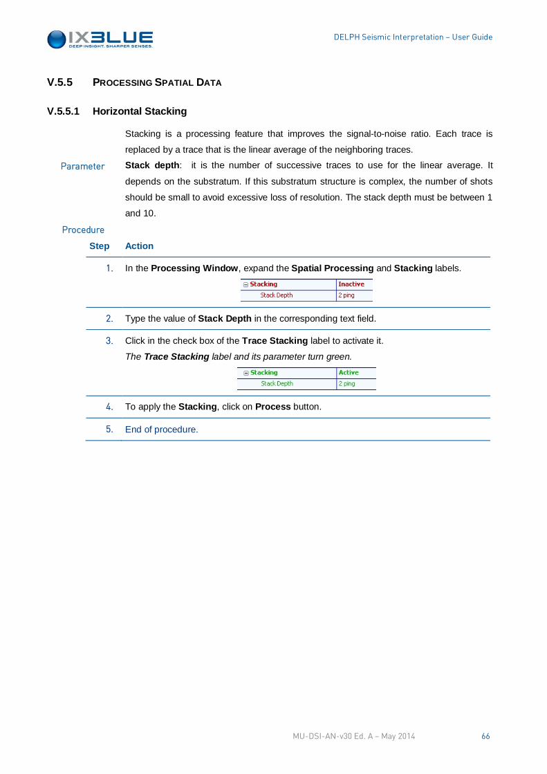
DELPH Seismic Interpretation – User Guide
V.5.5 PROCESSING SPATIAL DATA
V.5.5.1 Horizontal Stacking
Stacking is a processing feature that improves the signal-to-noise ratio. Each trace is
replaced by a trace that is the linear average of the neighboring traces.
Stack depth: it is the number of successive traces to use for the linear average. It
depends on the substratum. If this substratum structure is complex, the number of shots
should be small to avoid excessive loss of resolution. The stack depth must be between 1
and 10.
Step Action
1. In the Processing Window, expand the Spatial Processing and Stacking labels.
2. Type the value of Stack Depth in the corresponding text field.
3. Click in the check box of the Trace Stacking label to activate it.
The Trace Stacking label and its parameter turn green.
4. To apply the Stacking, click on Process button.
5. End of procedure.
Parameter
Procedure
MU-DSI-AN-v30 Ed. A – May 2014 66
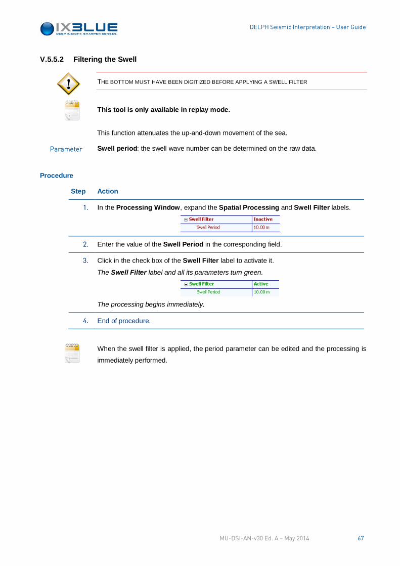
DELPH Seismic Interpretation – User Guide
V.5.5.2 Filtering the Swell
THE BOTTOM MUST HAVE BEEN DIGITIZED BEFORE APPLYING A SWELL FILTER
This tool is only available in replay mode.
This function attenuates the up-and-down movement of the sea.
Swell period: the swell wave number can be determined on the raw data.
Procedure
Step Action
1. In the Processing Window, expand the Spatial Processing and Swell Filter labels.
2. Enter the value of the Swell Period in the corresponding field.
3. Click in the check box of the Swell Filter label to activate it.
The Swell Filter label and all its parameters turn green.
The processing begins immediately.
4. End of procedure.
When the swell filter is applied, the period parameter can be edited and the processing is
immediately performed.
Parameter
MU-DSI-AN-v30 Ed. A – May 2014 67
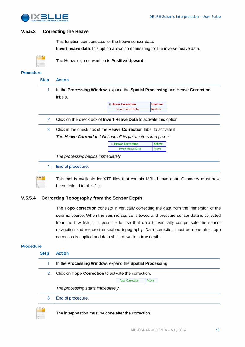
DELPH Seismic Interpretation – User Guide
V.5.5.3 Correcting the Heave
This function compensates for the heave sensor data.
Invert heave data: this option allows compensating for the inverse heave data.
The Heave sign convention is Positive Upward.
Procedure Step Action
1. In the Processing Window, expand the Spatial Processing and Heave Correction
labels.
2. Click on the check box of Invert Heave Data to activate this option.
3. Click in the check box of the Heave Correction label to activate it.
The Heave Correction label and all its parameters turn green.
The processing begins immediately.
4. End of procedure.
This tool is available for XTF files that contain MRU heave data. Geometry must have
been defined for this file.
V.5.5.4 Correcting Topography from the Sensor Depth
The Topo correction consists in vertically correcting the data from the immersion of the
seismic source. When the seismic source is towed and pressure sensor data is collected
from the tow fish, it is possible to use that data to vertically compensate the sensor
navigation and restore the seabed topography. Data correction must be done after topo
correction is applied and data shifts down to a true depth.
Procedure Step Action
1. In the Processing Window, expand the Spatial Processing.
2. Click on Topo Correction to activate the correction.
The processing starts immediately.
3. End of procedure.
The interpretation must be done after the correction.
MU-DSI-AN-v30 Ed. A – May 2014 68
DELPH Seismic Interpretation – User Guide
V.5.6 DETECTING THE BOTTOM AND THE REFLECTORS
The bottom and the reflectors can be detected manually and with the auto-tracking tool.
The auto-tracking tool is based on two methods: image and signal processing.
The auto tracking method is based on an image processing technique used in simple
pattern recognition. For the reflector/bottom tracking method, the reflector/bottom is
modeled with line segment. It is a trial-and-error method: from an initial point, the best (at
a statistical point of view) line segment (meter, time) is computed then the next point is
determined. This new point is used as initial point for the next computation and so on.
Depending on the gain correction and the noise in the data you may need to tune the
horizontal and vertical sensibility.
The second method is directly based on the signal. The bottom is detected with the help of
a vertical detection window.
V.5.6.1 Tracking the Bottom
The bottom auto-tracking is a very useful tool allowing the automatic digitalization of the
bottom in a seismic profile. You only have to initiate the digitalization and the auto tracking
follows the bottom until its end or until the end of the profile. It is working very efficiently in
situations where the bottom appears distinctively in the seismic profile.
Once activated, the bottom-tracking mode and manual is used in the Interpretation area.
• In the Image method, you have to define the size (vertical and horizontal) of the
detection window and the threshold level.
• In the Signal method, you have only to define the vertical detection window.
This section describes how to set up the parameters, see section V.6 for the application of
these parameters.
These parameters must be set up:
• Vertical Detection Window: corresponds to the length (in time) of the detection
window to use.
• Horizontal Detection Window: corresponds to the number of pings of the detection
window to use.
• Threshold level: it gives the detection threshold of the points to take into account for
the process. The calculation uses all the points the values of which overpass this
threshold multiplied by the maximum signal value. Default value is 15 %. Higher this
threshold is and more accurate the bottom is tracked but the tracking may stop more
often.
Swell detection must be de-activated before using bottom tracking.
Image Processing
Signal Processing
Parameters
MU-DSI-AN-v30 Ed. A – May 2014 69
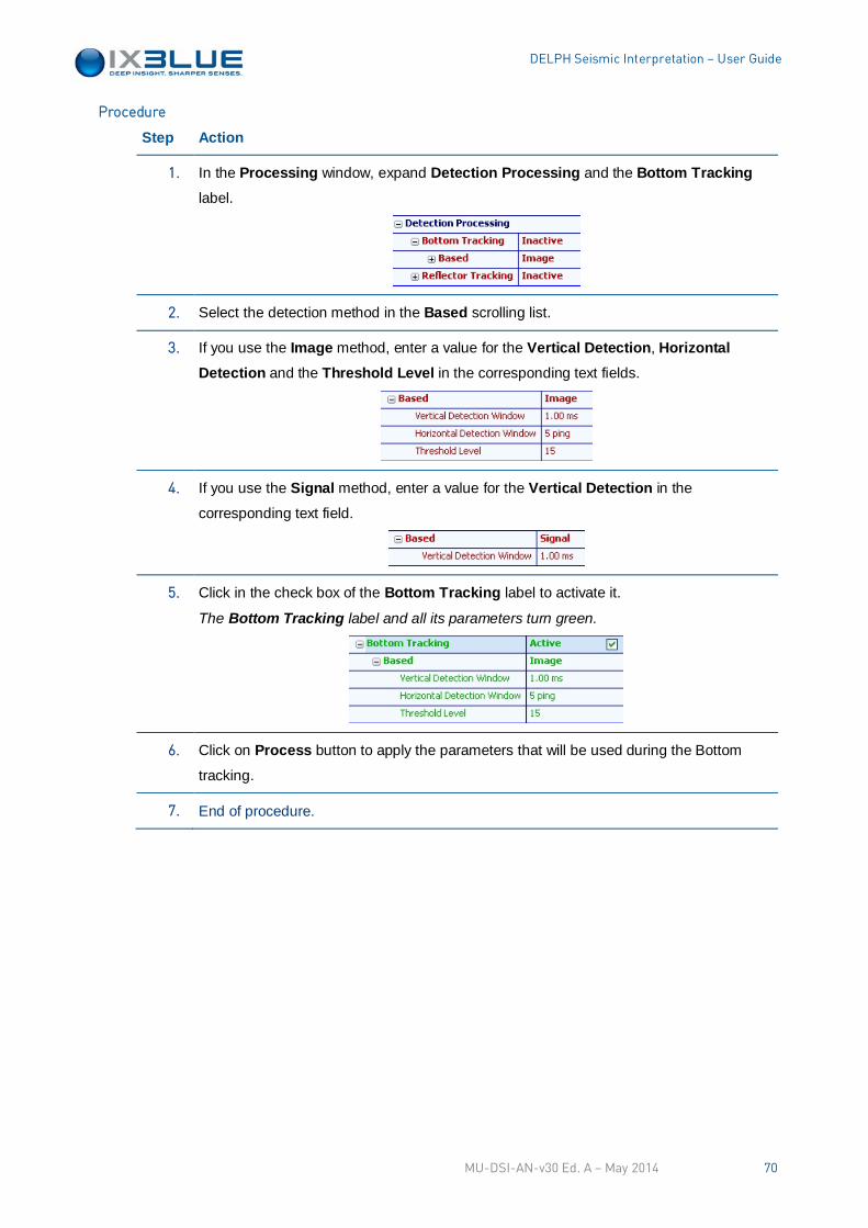
DELPH Seismic Interpretation – User Guide
Step Action
1. In the Processing window, expand Detection Processing and the Bottom Tracking
label.
2. Select the detection method in the Based scrolling list.
3. If you use the Image method, enter a value for the Vertical Detection, Horizontal Detection and the Threshold Level in the corresponding text fields.
4. If you use the Signal method, enter a value for the Vertical Detection in the
corresponding text field.
5. Click in the check box of the Bottom Tracking label to activate it.
The Bottom Tracking label and all its parameters turn green.
6. Click on Process button to apply the parameters that will be used during the Bottom
tracking.
7. End of procedure.
Procedure
MU-DSI-AN-v30 Ed. A – May 2014 70
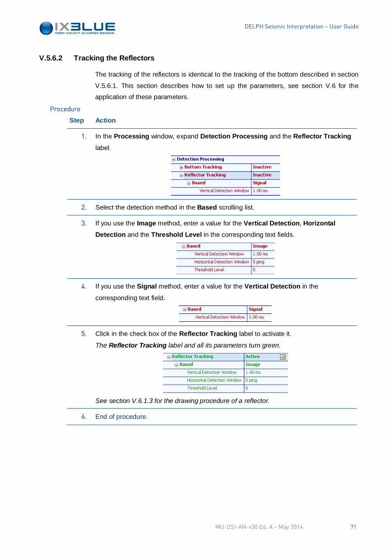
DELPH Seismic Interpretation – User Guide
V.5.6.2 Tracking the Reflectors
The tracking of the reflectors is identical to the tracking of the bottom described in section
V.5.6.1. This section describes how to set up the parameters, see section V.6 for the
application of these parameters.
Step Action
1. In the Processing window, expand Detection Processing and the Reflector Tracking
label.
2. Select the detection method in the Based scrolling list.
3. If you use the Image method, enter a value for the Vertical Detection, Horizontal Detection and the Threshold Level in the corresponding text fields.
4. If you use the Signal method, enter a value for the Vertical Detection in the
corresponding text field.
5. Click in the check box of the Reflector Tracking label to activate it.
The Reflector Tracking label and all its parameters turn green.
See section V.6.1.3 for the drawing procedure of a reflector.
6. End of procedure.
Procedure
MU-DSI-AN-v30 Ed. A – May 2014 71
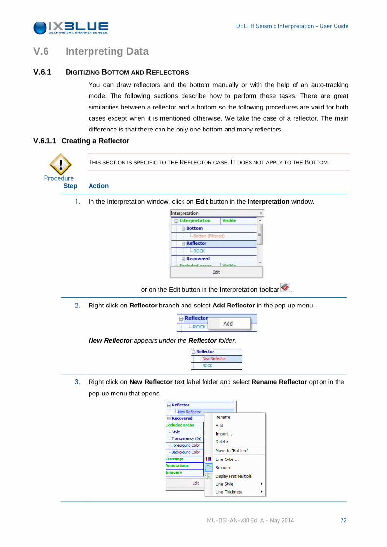
DELPH Seismic Interpretation – User Guide
V.6 Interpreting Data
V.6.1 DIGITIZING BOTTOM AND REFLECTORS You can draw reflectors and the bottom manually or with the help of an auto-tracking
mode. The following sections describe how to perform these tasks. There are great
similarities between a reflector and a bottom so the following procedures are valid for both
cases except when it is mentioned otherwise. We take the case of a reflector. The main
difference is that there can be only one bottom and many reflectors.
V.6.1.1 Creating a Reflector
THIS SECTION IS SPECIFIC TO THE REFLECTOR CASE. IT DOES NOT APPLY TO THE BOTTOM.
Step Action
1. In the Interpretation window, click on Edit button in the Interpretation window.
or on the Edit button in the Interpretation toolbar .
2. Right click on Reflector branch and select Add Reflector in the pop-up menu.
New Reflector appears under the Reflector folder.
3. Right click on New Reflector text label folder and select Rename Reflector option in the
pop-up menu that opens.
Procedure
MU-DSI-AN-v30 Ed. A – May 2014 72
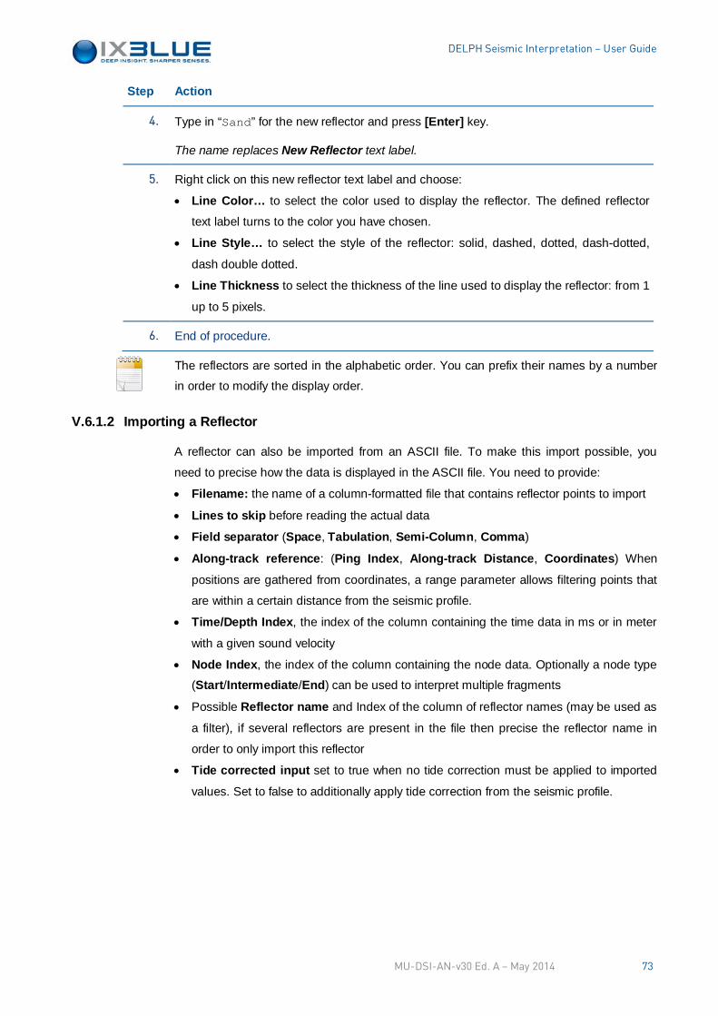
DELPH Seismic Interpretation – User Guide
Step Action
4. Type in “Sand” for the new reflector and press [Enter] key.
The name replaces New Reflector text label.
5. Right click on this new reflector text label and choose:
• Line Color… to select the color used to display the reflector. The defined reflector
text label turns to the color you have chosen.
• Line Style… to select the style of the reflector: solid, dashed, dotted, dash-dotted,
dash double dotted.
• Line Thickness to select the thickness of the line used to display the reflector: from 1
up to 5 pixels.
6. End of procedure.
The reflectors are sorted in the alphabetic order. You can prefix their names by a number
in order to modify the display order.
V.6.1.2 Importing a Reflector
A reflector can also be imported from an ASCII file. To make this import possible, you
need to precise how the data is displayed in the ASCII file. You need to provide:
• Filename: the name of a column-formatted file that contains reflector points to import
• Lines to skip before reading the actual data
• Field separator (Space, Tabulation, Semi-Column, Comma)
• Along-track reference: (Ping Index, Along-track Distance, Coordinates) When
positions are gathered from coordinates, a range parameter allows filtering points that
are within a certain distance from the seismic profile.
• Time/Depth Index, the index of the column containing the time data in ms or in meter
with a given sound velocity
• Node Index, the index of the column containing the node data. Optionally a node type
(Start/Intermediate/End) can be used to interpret multiple fragments
• Possible Reflector name and Index of the column of reflector names (may be used as
a filter), if several reflectors are present in the file then precise the reflector name in
order to only import this reflector
• Tide corrected input set to true when no tide correction must be applied to imported
values. Set to false to additionally apply tide correction from the seismic profile.
MU-DSI-AN-v30 Ed. A – May 2014 73
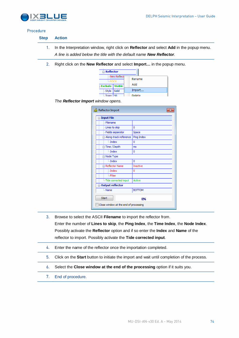
DELPH Seismic Interpretation – User Guide
Step Action
1. In the Interpretation window, right click on Reflector and select Add in the popup menu.
A line is added below the title with the default name New Reflector.
2. Right click on the New Reflector and select Import… in the popup menu.
The Reflector Import window opens.
3. Browse to select the ASCII Filename to import the reflector from.
Enter the number of Lines to skip, the Ping Index, the Time Index, the Node Index.
Possibly activate the Reflector option and if so enter the Index and Name of the
reflector to import. Possibly activate the Tide corrected input.
4. Enter the name of the reflector once the importation completed.
5. Click on the Start button to initiate the import and wait until completion of the process.
6. Select the Close window at the end of the processing option if it suits you.
7. End of procedure.
Procedure
MU-DSI-AN-v30 Ed. A – May 2014 74
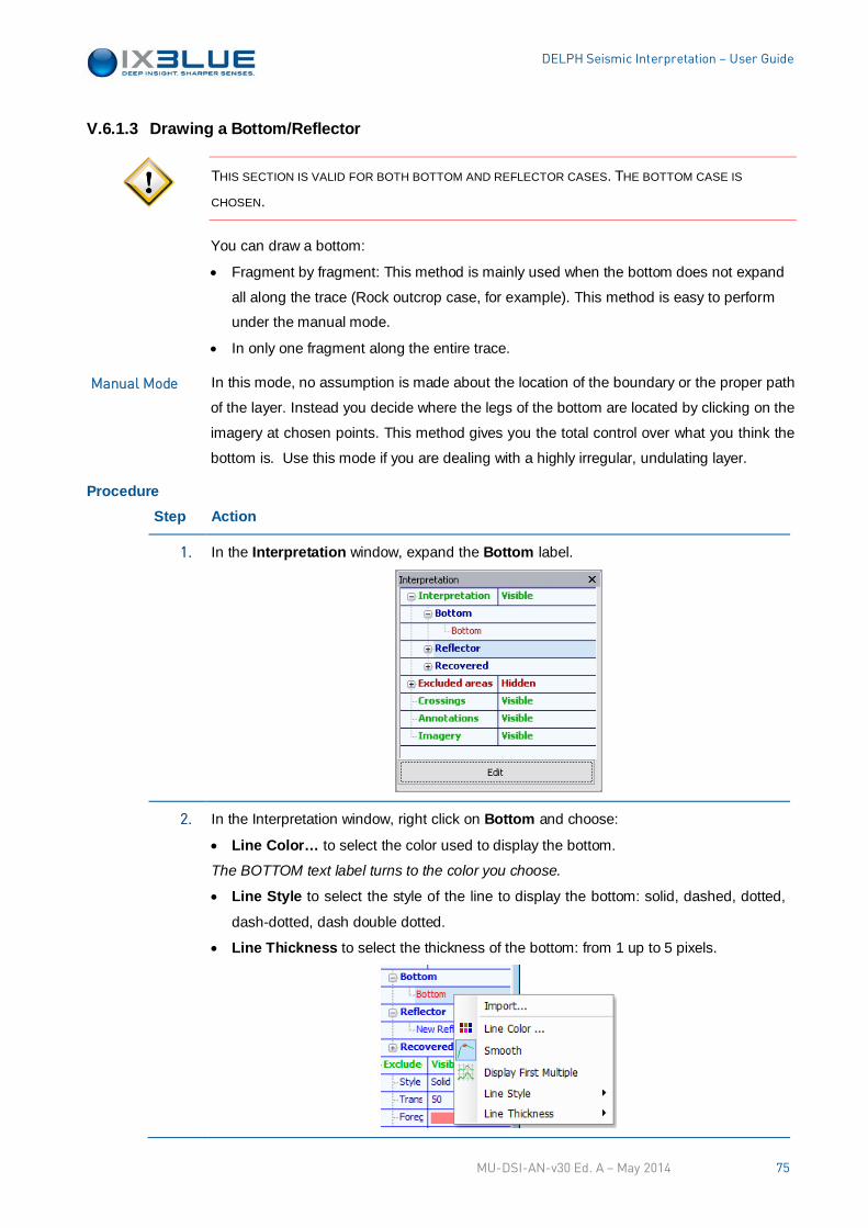
DELPH Seismic Interpretation – User Guide
V.6.1.3 Drawing a Bottom/Reflector
THIS SECTION IS VALID FOR BOTH BOTTOM AND REFLECTOR CASES. THE BOTTOM CASE IS
CHOSEN.
You can draw a bottom:
• Fragment by fragment: This method is mainly used when the bottom does not expand
all along the trace (Rock outcrop case, for example). This method is easy to perform
under the manual mode.
• In only one fragment along the entire trace.
In this mode, no assumption is made about the location of the boundary or the proper path
of the layer. Instead you decide where the legs of the bottom are located by clicking on the
imagery at chosen points. This method gives you the total control over what you think the
bottom is. Use this mode if you are dealing with a highly irregular, undulating layer.
Procedure Step Action
1. In the Interpretation window, expand the Bottom label.
2. In the Interpretation window, right click on Bottom and choose:
• Line Color… to select the color used to display the bottom.
The BOTTOM text label turns to the color you choose.
• Line Style to select the style of the line to display the bottom: solid, dashed, dotted,
dash-dotted, dash double dotted.
• Line Thickness to select the thickness of the bottom: from 1 up to 5 pixels.
Manual Mode
MU-DSI-AN-v30 Ed. A – May 2014 75
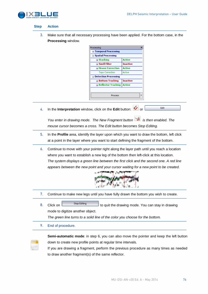
DELPH Seismic Interpretation – User Guide
Step Action
3. Make sure that all necessary processing have been applied. For the bottom case, in the Processing window.
4. In the Interpretation window, click on the Edit button: or
You enter in drawing mode. The New Fragment button is then enabled. The
mouse cursor becomes a cross. The Edit button becomes Stop Editing.
5. In the Profile area, identify the layer upon which you want to draw the bottom, left click
at a point in the layer where you want to start defining the fragment of the bottom.
6. Continue to move with your pointer right along the layer path until you reach a location
where you want to establish a new leg of the bottom then left-click at this location.
The system displays a green line between the first click and the second one. A red line
appears between the new point and your cursor waiting for a new point to be created.
7. Continue to make new legs until you have fully drawn the bottom you wish to create.
8. Click on to quit the drawing mode. You can stay in drawing
mode to digitize another object.
The green line turns to a solid line of the color you choose for the bottom.
9. End of procedure.
Semi-automatic mode: in step 6, you can also move the pointer and keep the left button
down to create new profile points at regular time intervals.
If you are drawing a fragment, perform the previous procedure as many times as needed
to draw another fragment(s) of the same reflector.
MU-DSI-AN-v30 Ed. A – May 2014 76
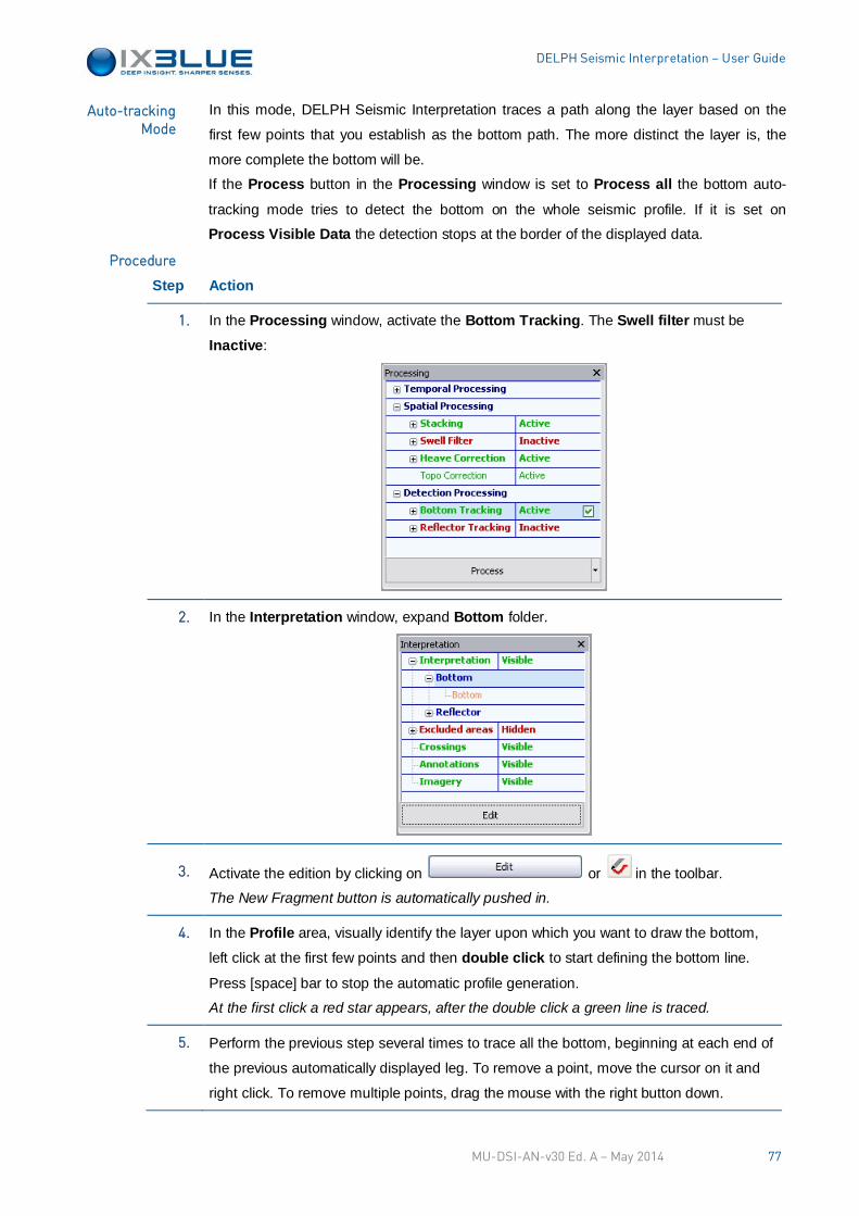
DELPH Seismic Interpretation – User Guide
In this mode, DELPH Seismic Interpretation traces a path along the layer based on the
first few points that you establish as the bottom path. The more distinct the layer is, the
more complete the bottom will be.
If the Process button in the Processing window is set to Process all the bottom auto-
tracking mode tries to detect the bottom on the whole seismic profile. If it is set on
Process Visible Data the detection stops at the border of the displayed data.
Step Action
1. In the Processing window, activate the Bottom Tracking. The Swell filter must be
Inactive:
2. In the Interpretation window, expand Bottom folder.
3. Activate the edition by clicking on or in the toolbar.
The New Fragment button is automatically pushed in.
4. In the Profile area, visually identify the layer upon which you want to draw the bottom,
left click at the first few points and then double click to start defining the bottom line.
Press [space] bar to stop the automatic profile generation.
At the first click a red star appears, after the double click a green line is traced.
5. Perform the previous step several times to trace all the bottom, beginning at each end of
the previous automatically displayed leg. To remove a point, move the cursor on it and
right click. To remove multiple points, drag the mouse with the right button down.
Auto-tracking Mode
Procedure
MU-DSI-AN-v30 Ed. A – May 2014 77
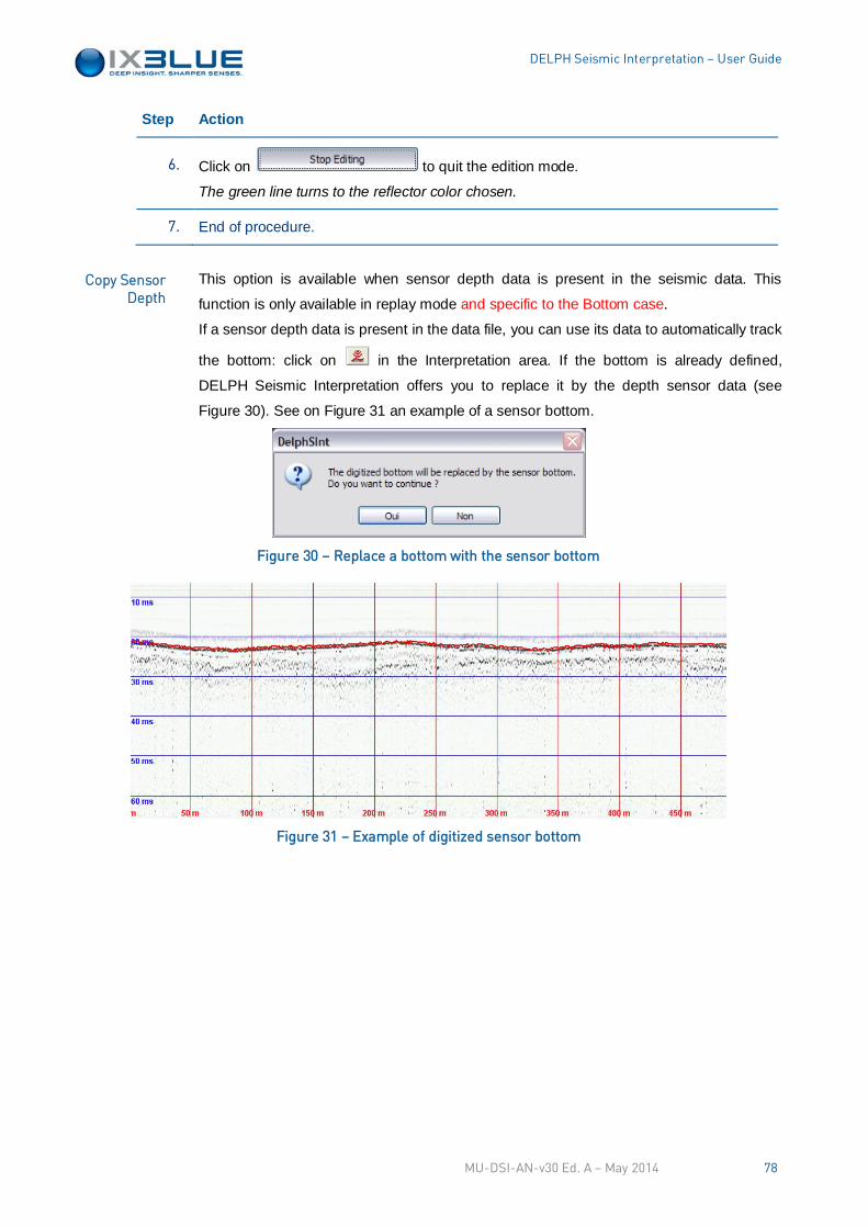
DELPH Seismic Interpretation – User Guide
Step Action
6. Click on to quit the edition mode.
The green line turns to the reflector color chosen.
7. End of procedure.
This option is available when sensor depth data is present in the seismic data. This
function is only available in replay mode and specific to the Bottom case.
If a sensor depth data is present in the data file, you can use its data to automatically track
the bottom: click on in the Interpretation area. If the bottom is already defined,
DELPH Seismic Interpretation offers you to replace it by the depth sensor data (see
Figure 30). See on Figure 31 an example of a sensor bottom.
Figure 30 – Replace a bottom with the sensor bottom
Figure 31 – Example of digitized sensor bottom
Copy Sensor Depth
MU-DSI-AN-v30 Ed. A – May 2014 78
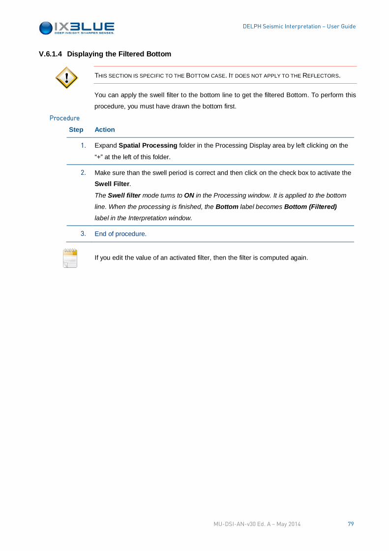
DELPH Seismic Interpretation – User Guide
V.6.1.4 Displaying the Filtered Bottom
THIS SECTION IS SPECIFIC TO THE BOTTOM CASE. IT DOES NOT APPLY TO THE REFLECTORS.
You can apply the swell filter to the bottom line to get the filtered Bottom. To perform this
procedure, you must have drawn the bottom first.
Step Action
1. Expand Spatial Processing folder in the Processing Display area by left clicking on the
“+” at the left of this folder.
2. Make sure than the swell period is correct and then click on the check box to activate the
Swell Filter.
The Swell filter mode turns to ON in the Processing window. It is applied to the bottom
line. When the processing is finished, the Bottom label becomes Bottom (Filtered) label in the Interpretation window.
3. End of procedure.
If you edit the value of an activated filter, then the filter is computed again.
Procedure
MU-DSI-AN-v30 Ed. A – May 2014 79
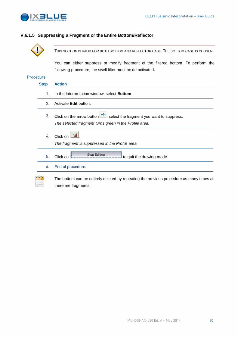
DELPH Seismic Interpretation – User Guide
V.6.1.5 Suppressing a Fragment or the Entire Bottom/Reflector
THIS SECTION IS VALID FOR BOTH BOTTOM AND REFLECTOR CASE. THE BOTTOM CASE IS CHOSEN.
You can either suppress or modify fragment of the filtered bottom. To perform the
following procedure, the swell filter must be de-activated.
Step Action
1. In the Interpretation window, select Bottom.
2. Activate Edit button.
3. Click on the arrow button , select the fragment you want to suppress.
The selected fragment turns green in the Profile area.
4. Click on .
The fragment is suppressed in the Profile area.
5. Click on to quit the drawing mode.
6. End of procedure.
The bottom can be entirely deleted by repeating the previous procedure as many times as
there are fragments.
Procedure
MU-DSI-AN-v30 Ed. A – May 2014 80
DELPH Seismic Interpretation – User Guide
V.6.1.6 Modifying a Bottom/Reflector Fragment
THIS SECTION IS VALID FOR BOTH BOTTOM AND REFLECTOR CASE. THE BOTTOM CASE IS CHOSEN.
You can either suppress or modify fragment of the filtered bottom. To perform the
following procedure, the swell filter must be de-activated.
Step Action
1. In the Interpretation window, select Bottom.
2. Activate the Edit button, select the fragment to modify with or .
The selected segment turns green in the Profile area.
3. • To add a new point: left click on the leg where you want to add a new point (you can
also add a new point before the first one or after the last one).
• To delete a point: select the point (a red rectangle appears) and right- click to delete.
• To delete several points: drag the mouse with the right button down over the points
that you want to remove.
• To modify the location of a point: left click on it, keep the left button pressed and
move to the new location, release the button to validate.
4. End of procedure.
Procedure
MU-DSI-AN-v30 Ed. A – May 2014 81
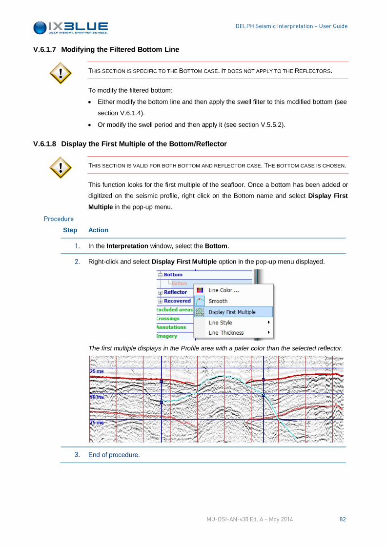
DELPH Seismic Interpretation – User Guide
V.6.1.7 Modifying the Filtered Bottom Line
THIS SECTION IS SPECIFIC TO THE BOTTOM CASE. IT DOES NOT APPLY TO THE REFLECTORS.
To modify the filtered bottom:
• Either modify the bottom line and then apply the swell filter to this modified bottom (see
section V.6.1.4).
• Or modify the swell period and then apply it (see section V.5.5.2).
V.6.1.8 Display the First Multiple of the Bottom/Reflector
THIS SECTION IS VALID FOR BOTH BOTTOM AND REFLECTOR CASE. THE BOTTOM CASE IS CHOSEN.
This function looks for the first multiple of the seafloor. Once a bottom has been added or
digitized on the seismic profile, right click on the Bottom name and select Display First Multiple in the pop-up menu.
Step Action
1. In the Interpretation window, select the Bottom.
2. Right-click and select Display First Multiple option in the pop-up menu displayed.
The first multiple displays in the Profile area with a paler color than the selected reflector.
3. End of procedure.
Procedure
MU-DSI-AN-v30 Ed. A – May 2014 82
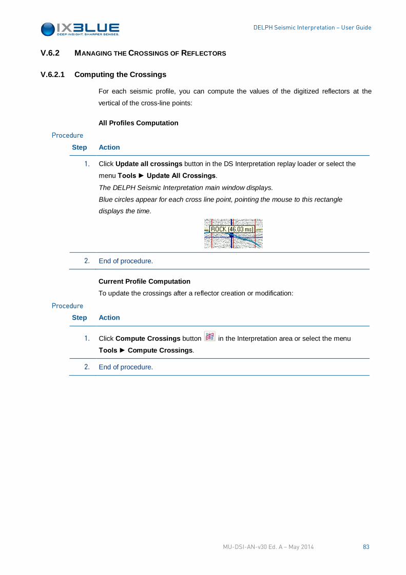
DELPH Seismic Interpretation – User Guide
V.6.2 MANAGING THE CROSSINGS OF REFLECTORS
V.6.2.1 Computing the Crossings
For each seismic profile, you can compute the values of the digitized reflectors at the
vertical of the cross-line points:
All Profiles Computation
Step Action
1. Click Update all crossings button in the DS Interpretation replay loader or select the
menu Tools ► Update All Crossings.
The DELPH Seismic Interpretation main window displays.
Blue circles appear for each cross line point, pointing the mouse to this rectangle
displays the time.
2. End of procedure.
Current Profile Computation To update the crossings after a reflector creation or modification:
Step Action
1. Click Compute Crossings button in the Interpretation area or select the menu
Tools ► Compute Crossings.
2. End of procedure.
Procedure
Procedure
MU-DSI-AN-v30 Ed. A – May 2014 83
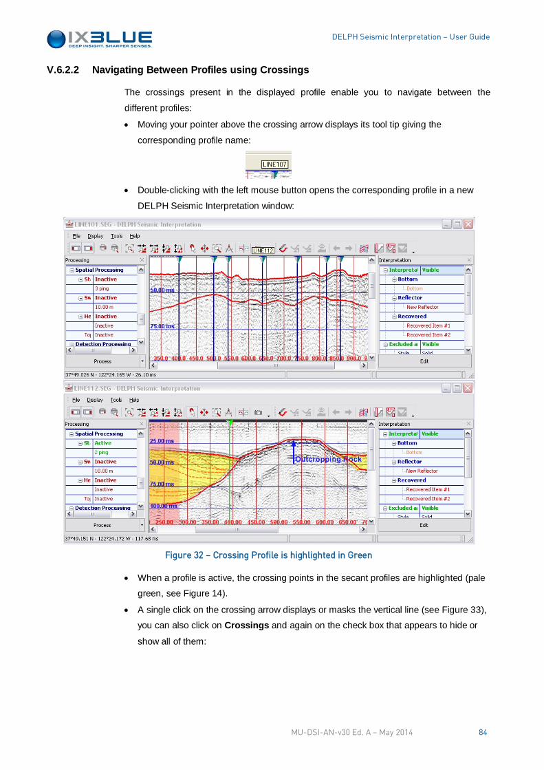
DELPH Seismic Interpretation – User Guide
V.6.2.2 Navigating Between Profiles using Crossings
The crossings present in the displayed profile enable you to navigate between the
different profiles:
• Moving your pointer above the crossing arrow displays its tool tip giving the
corresponding profile name:
• Double-clicking with the left mouse button opens the corresponding profile in a new
DELPH Seismic Interpretation window:
Figure 32 – Crossing Profile is highlighted in Green
• When a profile is active, the crossing points in the secant profiles are highlighted (pale
green, see Figure 14).
• A single click on the crossing arrow displays or masks the vertical line (see Figure 33),
you can also click on Crossings and again on the check box that appears to hide or
show all of them:
MU-DSI-AN-v30 Ed. A – May 2014 84
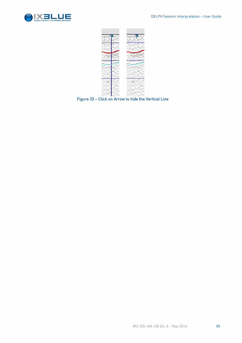
DELPH Seismic Interpretation – User Guide
Figure 33 – Click on Arrow to hide the Vertical Line
MU-DSI-AN-v30 Ed. A – May 2014 85
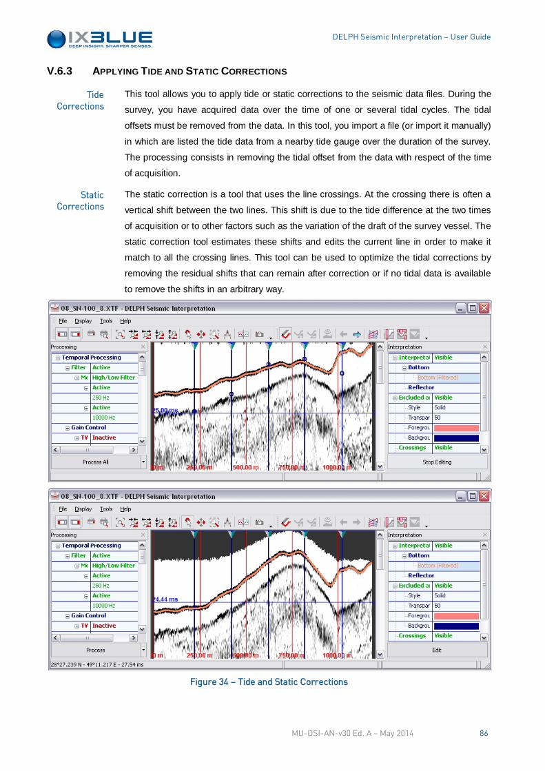
DELPH Seismic Interpretation – User Guide
V.6.3 APPLYING TIDE AND STATIC CORRECTIONS
This tool allows you to apply tide or static corrections to the seismic data files. During the
survey, you have acquired data over the time of one or several tidal cycles. The tidal
offsets must be removed from the data. In this tool, you import a file (or import it manually)
in which are listed the tide data from a nearby tide gauge over the duration of the survey.
The processing consists in removing the tidal offset from the data with respect of the time
of acquisition.
The static correction is a tool that uses the line crossings. At the crossing there is often a
vertical shift between the two lines. This shift is due to the tide difference at the two times
of acquisition or to other factors such as the variation of the draft of the survey vessel. The
static correction tool estimates these shifts and edits the current line in order to make it
match to all the crossing lines. This tool can be used to optimize the tidal corrections by
removing the residual shifts that can remain after correction or if no tidal data is available
to remove the shifts in an arbitrary way.
Figure 34 – Tide and Static Corrections
Tide Corrections
Static Corrections
MU-DSI-AN-v30 Ed. A – May 2014 86
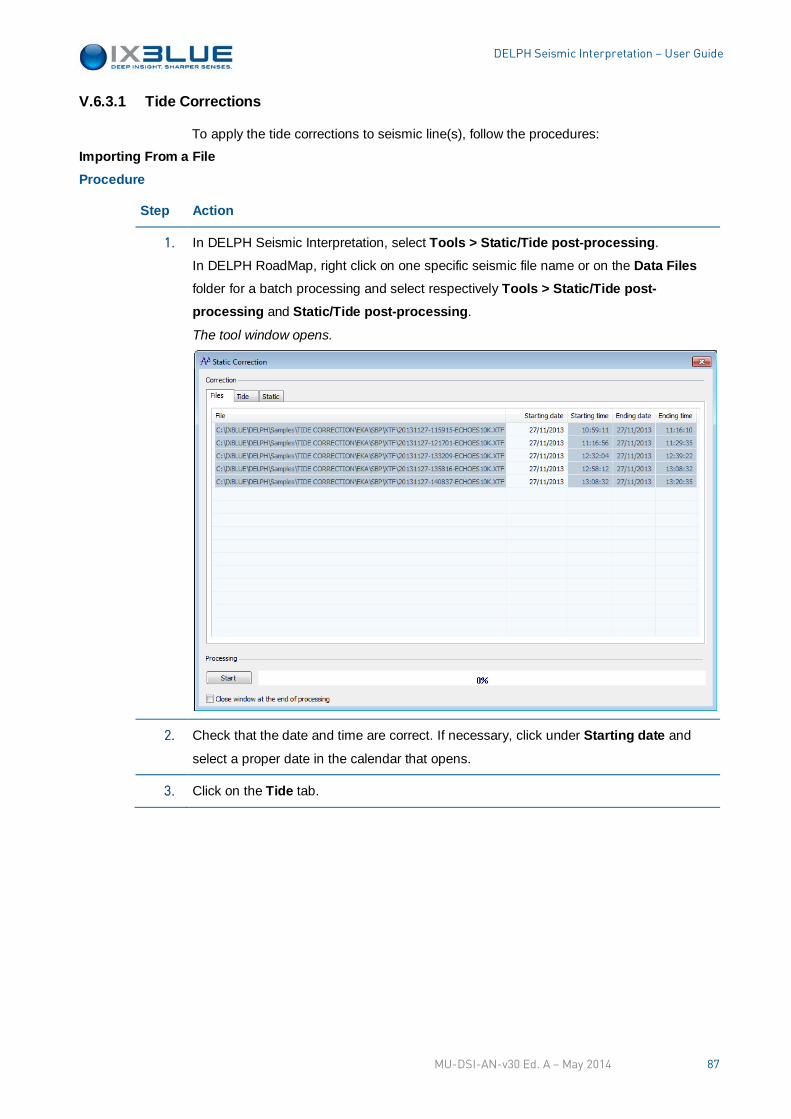
DELPH Seismic Interpretation – User Guide
V.6.3.1 Tide Corrections
To apply the tide corrections to seismic line(s), follow the procedures:
Importing From a File Procedure
Step Action
1. In DELPH Seismic Interpretation, select Tools > Static/Tide post-processing.
In DELPH RoadMap, right click on one specific seismic file name or on the Data Files
folder for a batch processing and select respectively Tools > Static/Tide post-processing and Static/Tide post-processing.
The tool window opens.
2. Check that the date and time are correct. If necessary, click under Starting date and
select a proper date in the calendar that opens.
3. Click on the Tide tab.
MU-DSI-AN-v30 Ed. A – May 2014 87
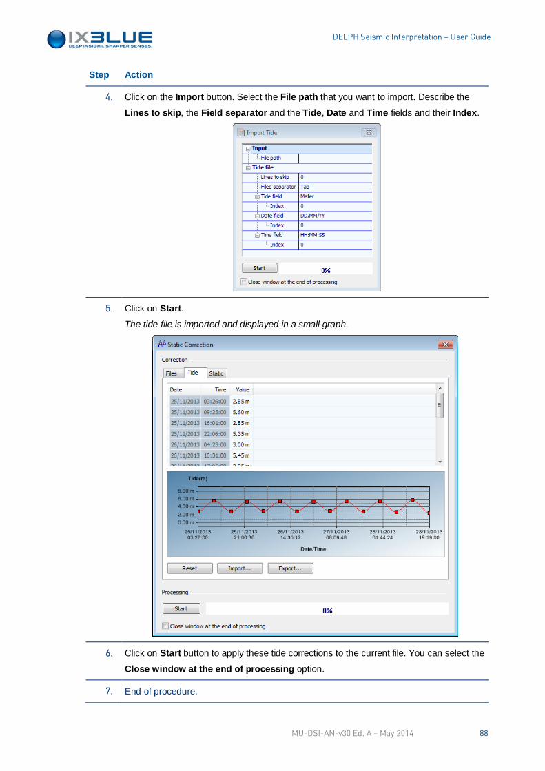
DELPH Seismic Interpretation – User Guide
Step Action
4. Click on the Import button. Select the File path that you want to import. Describe the
Lines to skip, the Field separator and the Tide, Date and Time fields and their Index.
5. Click on Start. The tide file is imported and displayed in a small graph.
6. Click on Start button to apply these tide corrections to the current file. You can select the
Close window at the end of processing option.
7. End of procedure.
MU-DSI-AN-v30 Ed. A – May 2014 88
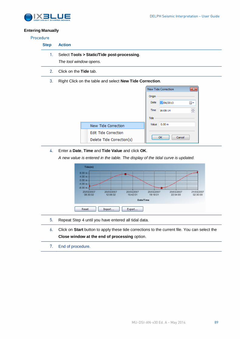
DELPH Seismic Interpretation – User Guide
Entering Manually
Step Action
1. Select Tools > Static/Tide post-processing.
The tool window opens.
2. Click on the Tide tab.
3. Right Click on the table and select New Tide Correction.
4. Enter a Date, Time and Tide Value and click OK.
A new value is entered in the table. The display of the tidal curve is updated.
5. Repeat Step 4 until you have entered all tidal data.
6. Click on Start button to apply these tide corrections to the current file. You can select the
Close window at the end of processing option.
7. End of procedure.
Procedure
MU-DSI-AN-v30 Ed. A – May 2014 89
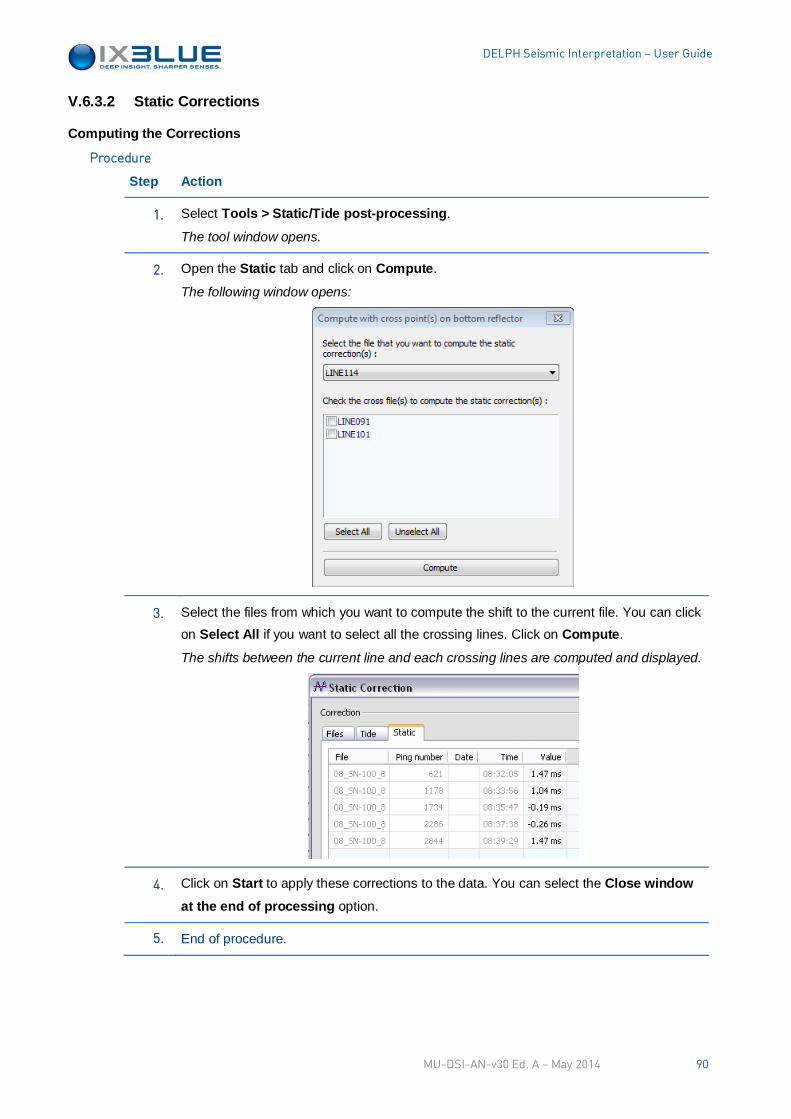
DELPH Seismic Interpretation – User Guide
V.6.3.2 Static Corrections
Computing the Corrections
Step Action
1. Select Tools > Static/Tide post-processing.
The tool window opens.
2. Open the Static tab and click on Compute.
The following window opens:
3. Select the files from which you want to compute the shift to the current file. You can click on Select All if you want to select all the crossing lines. Click on Compute.
The shifts between the current line and each crossing lines are computed and displayed.
4. Click on Start to apply these corrections to the data. You can select the Close window at the end of processing option.
5. End of procedure.
Procedure
MU-DSI-AN-v30 Ed. A – May 2014 90
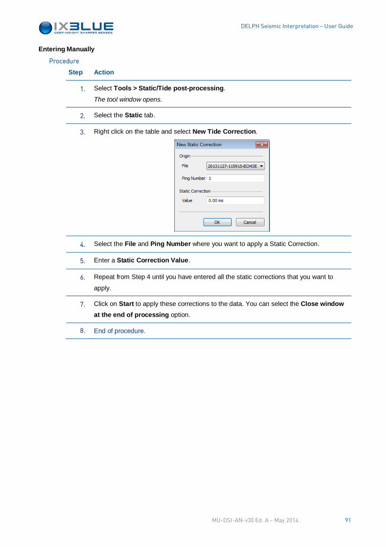
DELPH Seismic Interpretation – User Guide
Entering Manually
Step Action
1. Select Tools > Static/Tide post-processing.
The tool window opens.
2. Select the Static tab.
3. Right click on the table and select New Tide Correction.
4. Select the File and Ping Number where you want to apply a Static Correction.
5. Enter a Static Correction Value.
6. Repeat from Step 4 until you have entered all the static corrections that you want to
apply.
7. Click on Start to apply these corrections to the data. You can select the Close window at the end of processing option.
8. End of procedure.
Procedure
MU-DSI-AN-v30 Ed. A – May 2014 91
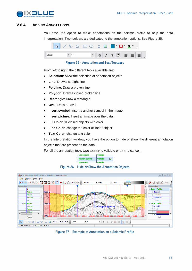
DELPH Seismic Interpretation – User Guide
V.6.4 ADDING ANNOTATIONS
You have the option to make annotations on the seismic profile to help the data
interpretation. Two toolbars are dedicated to the annotation options. See Figure 35.
Figure 35 - Annotation and Text Toolbars
From left to right, the different tools available are:
• Selection: Allow the selection of annotation objects
• Line: Draw a straight line
• Polyline: Draw a broken line
• Polygon: Draw a closed broken line
• Rectangle: Draw a rectangle
• Oval: Draw an oval
• Insert symbol: Insert a anchor symbol in the image
• Insert picture: Insert an image over the data
• Fill Color: fill closed objects with color
• Line Color: change the color of linear object
• Text Color: change text color
In the Interpretation window, you have the option to hide or show the different annotation
objects that are present on the data.
For all the annotation tools type Enter to validate or Esc to cancel.
Figure 36 – Hide or Show the Annotation Objects
Figure 37 – Example of Annotation on a Seismic Profile
MU-DSI-AN-v30 Ed. A – May 2014 92
DELPH Seismic Interpretation – User Guide
V.6.4.1 Selecting Objects
The selection of annotation objects is made with the pointer tool . This tool allows
many operations on the objects.
Selecting Multiple Objects
Step Action
1. Left click to select the first object.
2. Press [Shift] and left click on the second object.
The two objects are both selected. Operations can be applied on both objects.
3. End of procedure.
Selecting Overlapping Objects
Step Action
1. Left click to select the object in the foreground.
2. Repeat the left click to select one after the other the objects behind the first one.
3. End of procedure.
Moving Objects
Step Action
1. Left click on the object to select it.
2. Left click on the selected object and do not release the mouse button.
3. Move the mouse to another location.
The object follows the mouse.
4. Release the mouse button when you have reached the location of your choice.
5. End of procedure.
Procedure
Procedure
Procedure
MU-DSI-AN-v30 Ed. A – May 2014 93
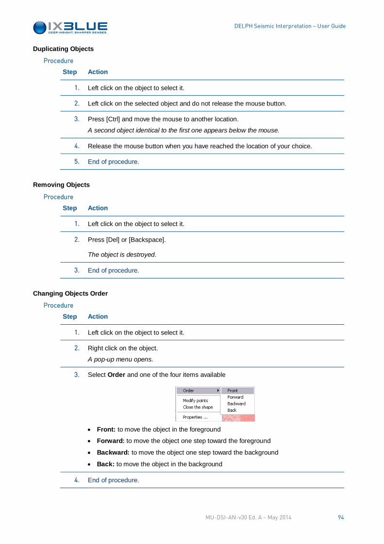
DELPH Seismic Interpretation – User Guide
Duplicating Objects
Step Action
1. Left click on the object to select it.
2. Left click on the selected object and do not release the mouse button.
3. Press [Ctrl] and move the mouse to another location.
A second object identical to the first one appears below the mouse.
4. Release the mouse button when you have reached the location of your choice.
5. End of procedure.
Removing Objects
Step Action
1. Left click on the object to select it.
2. Press [Del] or [Backspace].
The object is destroyed.
3. End of procedure.
Changing Objects Order
Step Action
1. Left click on the object to select it.
2. Right click on the object.
A pop-up menu opens.
3. Select Order and one of the four items available
• Front: to move the object in the foreground
• Forward: to move the object one step toward the foreground
• Backward: to move the object one step toward the background
• Back: to move the object in the background
4. End of procedure.
Procedure
Procedure
Procedure
MU-DSI-AN-v30 Ed. A – May 2014 94
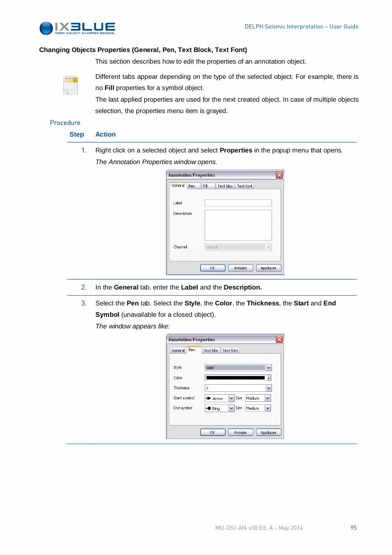
DELPH Seismic Interpretation – User Guide
Changing Objects Properties (General, Pen, Text Block, Text Font)
This section describes how to edit the properties of an annotation object.
Different tabs appear depending on the type of the selected object. For example, there is
no Fill properties for a symbol object.
The last applied properties are used for the next created object. In case of multiple objects
selection, the properties menu item is grayed.
Step Action
1. Right click on a selected object and select Properties in the popup menu that opens.
The Annotation Properties window opens.
2. In the General tab, enter the Label and the Description.
3. Select the Pen tab. Select the Style, the Color, the Thickness, the Start and End Symbol (unavailable for a closed object).
The window appears like:
Procedure
MU-DSI-AN-v30 Ed. A – May 2014 95
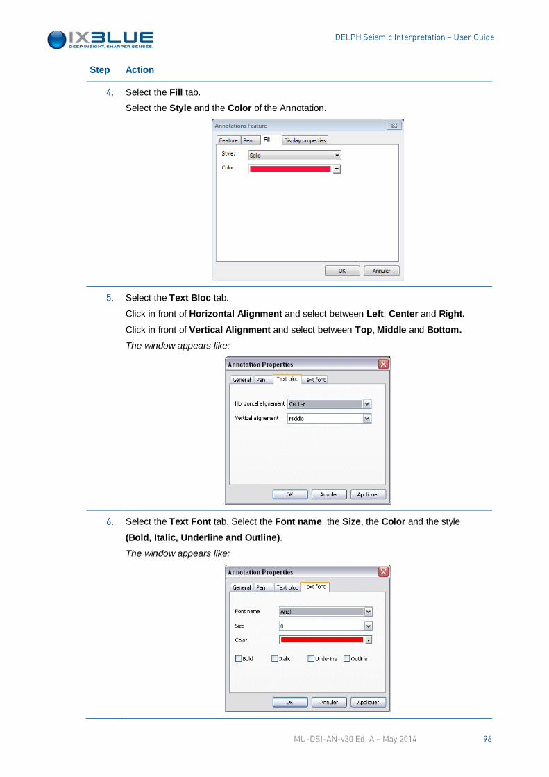
DELPH Seismic Interpretation – User Guide
Step Action
4. Select the Fill tab.
Select the Style and the Color of the Annotation.
5. Select the Text Bloc tab.
Click in front of Horizontal Alignment and select between Left, Center and Right. Click in front of Vertical Alignment and select between Top, Middle and Bottom. The window appears like:
6. Select the Text Font tab. Select the Font name, the Size, the Color and the style (Bold, Italic, Underline and Outline). The window appears like:
MU-DSI-AN-v30 Ed. A – May 2014 96
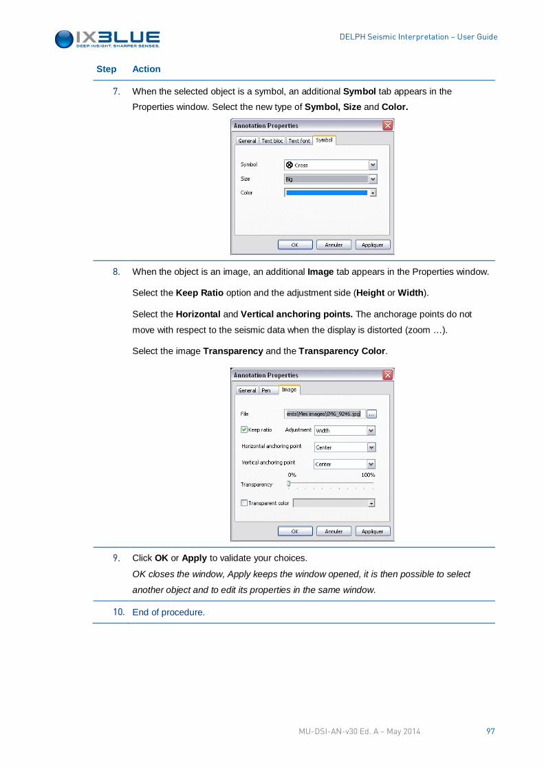
DELPH Seismic Interpretation – User Guide
Step Action
7. When the selected object is a symbol, an additional Symbol tab appears in the
Properties window. Select the new type of Symbol, Size and Color.
8. When the object is an image, an additional Image tab appears in the Properties window.
Select the Keep Ratio option and the adjustment side (Height or Width).
Select the Horizontal and Vertical anchoring points. The anchorage points do not
move with respect to the seismic data when the display is distorted (zoom …).
Select the image Transparency and the Transparency Color.
9. Click OK or Apply to validate your choices.
OK closes the window, Apply keeps the window opened, it is then possible to select
another object and to edit its properties in the same window.
10. End of procedure.
MU-DSI-AN-v30 Ed. A – May 2014 97
DELPH Seismic Interpretation – User Guide
V.6.4.2 Drawing Straight Lines
Step Action
1. Select the Straight Line tool .
2. Left click and drag the mouse to another location.
3. Release the mouse button.
A straight line is drawn between the location where you clicked first and the location
where you released the mouse.
4. End of procedure.
V.6.4.3 Drawing Poly-lines
Step Action
1. Select the Poly-line tool
2. Left click, release the mouse button and move the mouse to another location.
A first segment appears.
3. Repeat the step 1 to add points to the poly-line as many times as needed.
4. Double click to terminate the poly-line.
5. End of procedure.
V.6.4.4 Drawing Polygons
Step Action
1. Select the Polygon tool .
2. Left click, release the mouse button and move the mouse to another location.
A first segment appears.
3. Repeat the step 1 to add points to the polygon as many times as needed.
The last point added is linked to the first point of your polygon.
4. Double click to terminate the polygon.
5. End of procedure.
Procedure
Procedure
Procedure
MU-DSI-AN-v30 Ed. A – May 2014 98
DELPH Seismic Interpretation – User Guide
V.6.4.5 Drawing Rectangles
Step Action
1. Select the Rectangle tool .
2. Left click and drag the mouse to define the size of the rectangle.
3. Release the mouse button.
A rectangle is drawn between the location where you clicked first and the location where
you released the mouse.
4. End of procedure.
V.6.4.6 Drawing Ellipses
Step Action
1. Select the Ellipse tool .
2. Left click and drag the mouse to define the size of the ellipse.
3. Release the mouse button.
An ellipse is drawn between the location where you clicked first and the location where
you released the mouse.
4. End of procedure.
V.6.4.7 Inserting Symbols
Step Action
1. Select the Symbol tool .
2. Click in the display area at the place where you want to insert the symbol.
The default symbol appears at the location where you have clicked.
3. End of procedure.
Procedure
Procedure
Procedure
MU-DSI-AN-v30 Ed. A – May 2014 99
DELPH Seismic Interpretation – User Guide
V.6.4.8 Inserting Images
Step Action
1. Select the Image tool .
2. Click in the display area at the place where you want to insert the image.
The File Open window opens.
3. Browse the folders to select the image file to insert in the display.
4. Click OK.
The image is inserted in the display area.
5. Adjust the size of the image by shifting the sides with the mouse.
6. End of procedure.
V.6.4.9 Customizing Color
The color can be affected to all objects in three different ways. The operator can fill an
object with color, change the contour color of a linear object and change the color of an
object label. The color properties are also available in the Properties Window.
Step Action
1. Select the closed object (Polygon, Rectangle, Ellipse) from which you want to change
the color.
2. Click on the Fill Color tool and select the color in the palette that opens.
The object changes color.
3. End of procedure.
Step Action
1. Select the linear object (Straight Line, Polyline) from which you want to change the
color.
2. Click on the Pen Color tool and select the color in the palette that opens.
The linear object changes color.
3. End of procedure.
Procedure
Closed Object
Linear Object
MU-DSI-AN-v30 Ed. A – May 2014 100
DELPH Seismic Interpretation – User Guide
Step Action
1. Select the object from which you want to change the label color.
2. Click on the Text Color tool and select the color in the palette that opens.
The object changes color.
3. End of procedure.
V.6.4.10 Customizing Text
Step Action
1. Select the object of which you want to change the font, size, style and alignment.
2. Select a font, a size, a style or a alignment in the text toolbar.
The text changes.
3. End of procedure.
V.6.4.11 Customizing Shapes
Right click on the Poly-line and select Close the shape in the pop-up menu to transform
the poly-line into a polygon.
Right click on the Polygon and select Open the shape in the pop-up menu to transform
the polygon into a poly-line.
It is possible to move one or several points of a Poly-line, Polygon or Segment already
created. Right click on the shape, select Modify Points, click on the point that you want to
move and slide it to its new location.
Text Object
Procedure
Closing a Poly-line
Opening a Polygon
Moving points
MU-DSI-AN-v30 Ed. A – May 2014 101
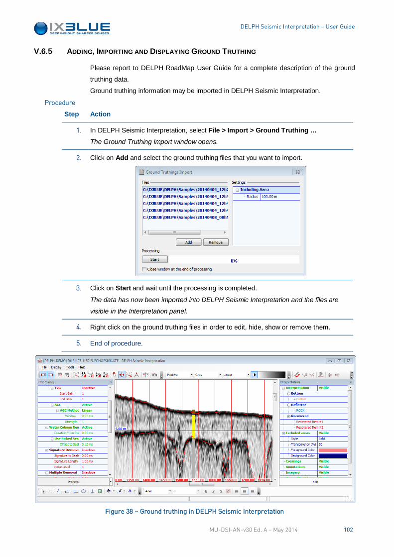
DELPH Seismic Interpretation – User Guide
V.6.5 ADDING, IMPORTING AND DISPLAYING GROUND TRUTHING
Please report to DELPH RoadMap User Guide for a complete description of the ground
truthing data.
Ground truthing information may be imported in DELPH Seismic Interpretation.
Step Action
1. In DELPH Seismic Interpretation, select File > Import > Ground Truthing … The Ground Truthing Import window opens.
2. Click on Add and select the ground truthing files that you want to import.
3. Click on Start and wait until the processing is completed.
The data has now been imported into DELPH Seismic Interpretation and the files are
visible in the Interpretation panel.
4. Right click on the ground truthing files in order to edit, hide, show or remove them.
5. End of procedure.
Figure 38 – Ground truthing in DELPH Seismic Interpretation
Procedure
MU-DSI-AN-v30 Ed. A – May 2014 102
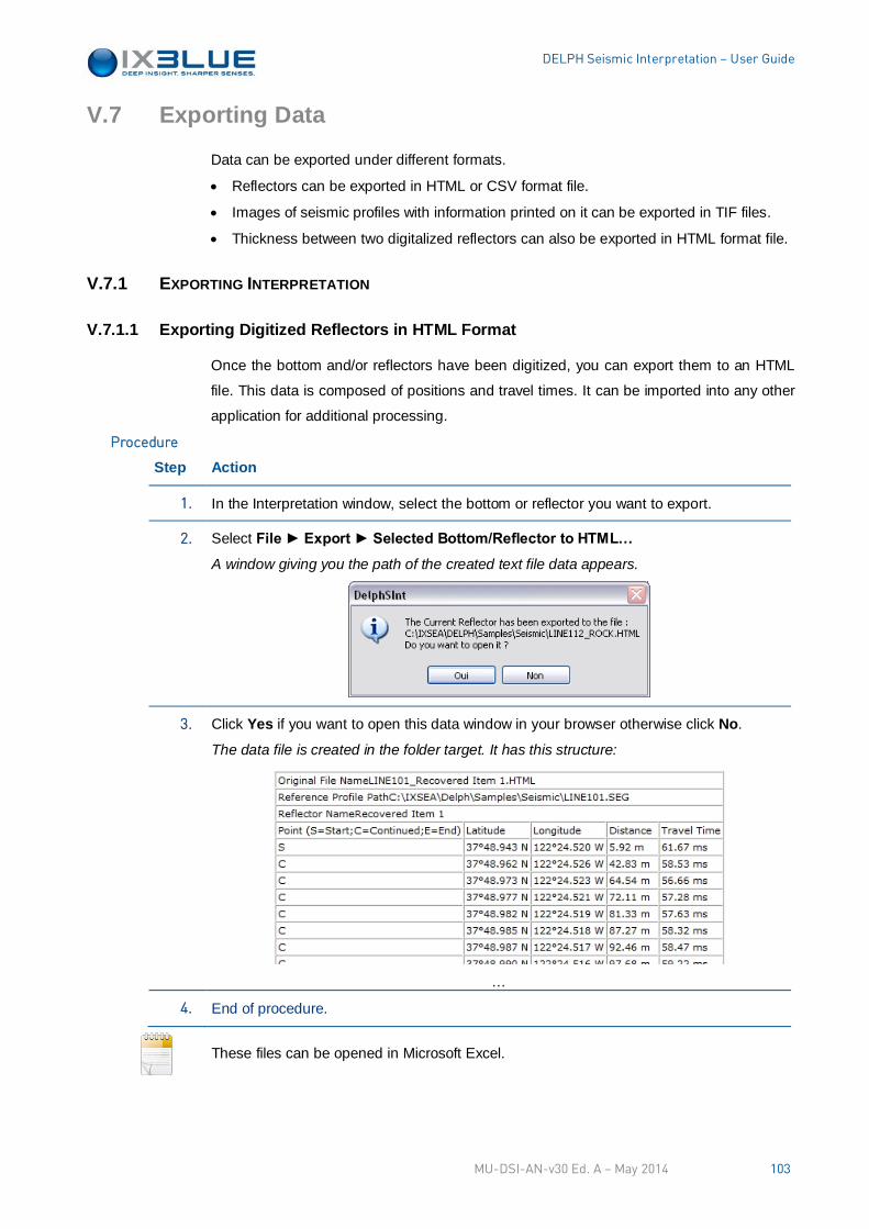
DELPH Seismic Interpretation – User Guide
V.7 Exporting Data
Data can be exported under different formats.
• Reflectors can be exported in HTML or CSV format file.
• Images of seismic profiles with information printed on it can be exported in TIF files.
• Thickness between two digitalized reflectors can also be exported in HTML format file.
V.7.1 EXPORTING INTERPRETATION
V.7.1.1 Exporting Digitized Reflectors in HTML Format
Once the bottom and/or reflectors have been digitized, you can export them to an HTML
file. This data is composed of positions and travel times. It can be imported into any other
application for additional processing.
Step Action
1. In the Interpretation window, select the bottom or reflector you want to export.
2. Select File ► Export ► Selected Bottom/Reflector to HTML…
A window giving you the path of the created text file data appears.
3. Click Yes if you want to open this data window in your browser otherwise click No.
The data file is created in the folder target. It has this structure:
…
4. End of procedure.
These files can be opened in Microsoft Excel.
Procedure
MU-DSI-AN-v30 Ed. A – May 2014 103
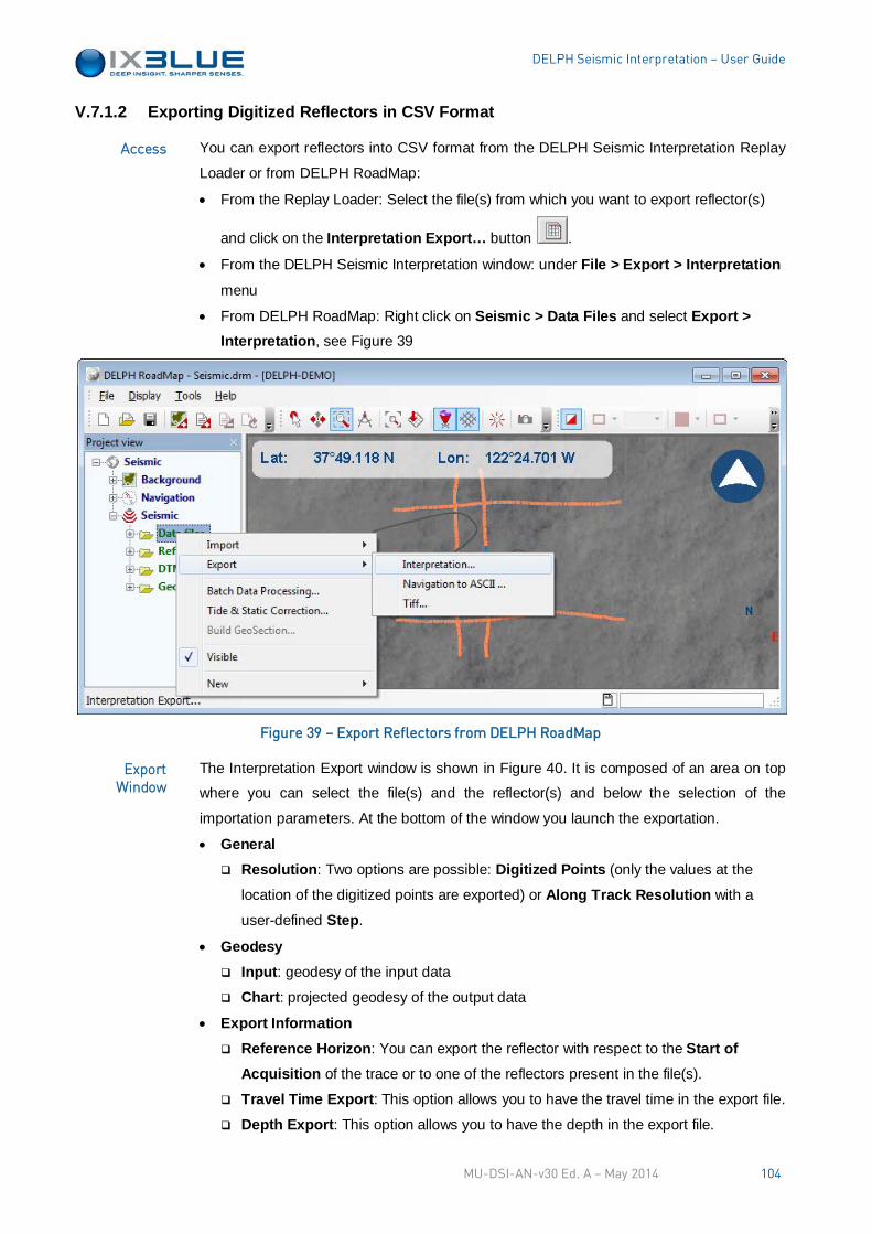
DELPH Seismic Interpretation – User Guide
V.7.1.2 Exporting Digitized Reflectors in CSV Format
You can export reflectors into CSV format from the DELPH Seismic Interpretation Replay
Loader or from DELPH RoadMap:
• From the Replay Loader: Select the file(s) from which you want to export reflector(s)
and click on the Interpretation Export… button .
• From the DELPH Seismic Interpretation window: under File > Export > Interpretation
menu
• From DELPH RoadMap: Right click on Seismic > Data Files and select Export > Interpretation, see Figure 39
Figure 39 – Export Reflectors from DELPH RoadMap
The Interpretation Export window is shown in Figure 40. It is composed of an area on top
where you can select the file(s) and the reflector(s) and below the selection of the
importation parameters. At the bottom of the window you launch the exportation.
• General Resolution: Two options are possible: Digitized Points (only the values at the
location of the digitized points are exported) or Along Track Resolution with a
user-defined Step.
• Geodesy Input: geodesy of the input data
Chart: projected geodesy of the output data
• Export Information Reference Horizon: You can export the reflector with respect to the Start of
Acquisition of the trace or to one of the reflectors present in the file(s).
Travel Time Export: This option allows you to have the travel time in the export file.
Depth Export: This option allows you to have the depth in the export file.
Access
Export Window
MU-DSI-AN-v30 Ed. A – May 2014 104
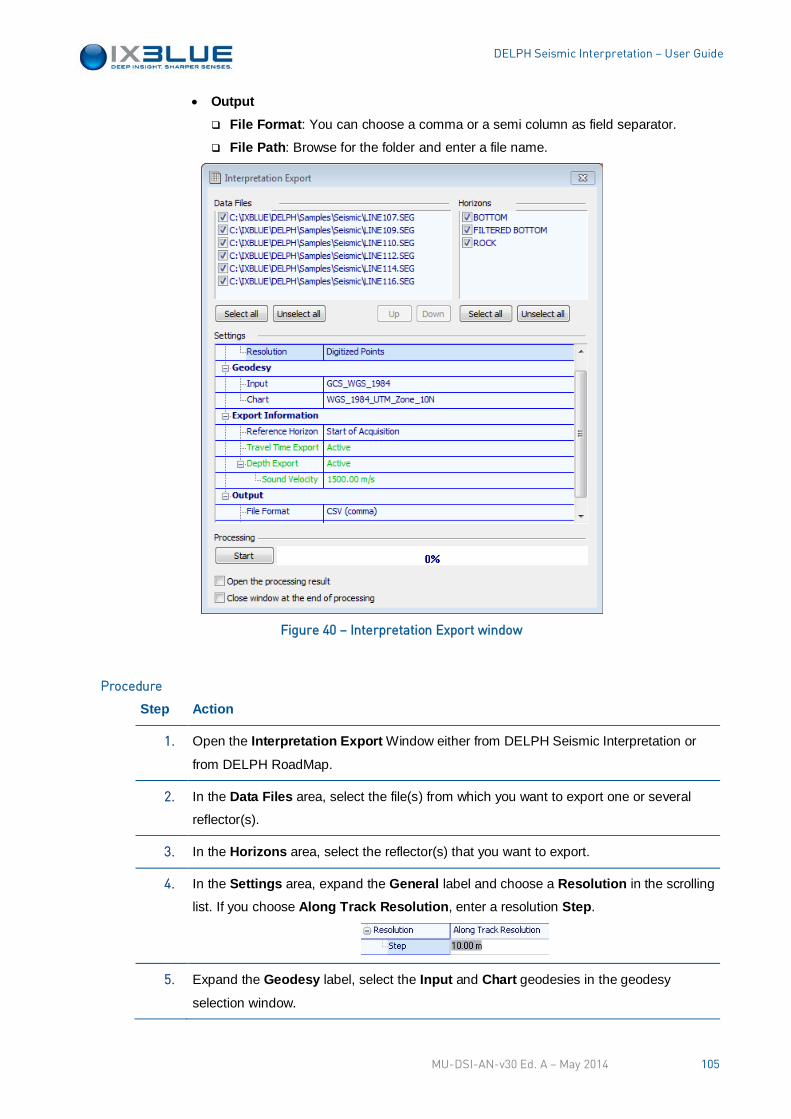
DELPH Seismic Interpretation – User Guide
• Output File Format: You can choose a comma or a semi column as field separator.
File Path: Browse for the folder and enter a file name.
Figure 40 – Interpretation Export window
Step Action
1. Open the Interpretation Export Window either from DELPH Seismic Interpretation or
from DELPH RoadMap.
2. In the Data Files area, select the file(s) from which you want to export one or several
reflector(s).
3. In the Horizons area, select the reflector(s) that you want to export.
4. In the Settings area, expand the General label and choose a Resolution in the scrolling
list. If you choose Along Track Resolution, enter a resolution Step.
5. Expand the Geodesy label, select the Input and Chart geodesies in the geodesy
selection window.
Procedure
MU-DSI-AN-v30 Ed. A – May 2014 105
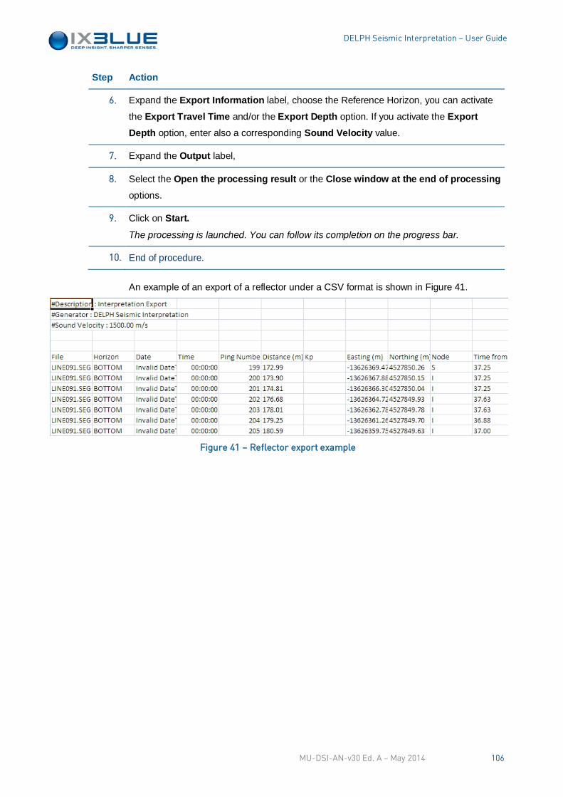
DELPH Seismic Interpretation – User Guide
Step Action
6. Expand the Export Information label, choose the Reference Horizon, you can activate
the Export Travel Time and/or the Export Depth option. If you activate the Export Depth option, enter also a corresponding Sound Velocity value.
7. Expand the Output label,
8. Select the Open the processing result or the Close window at the end of processing
options.
9. Click on Start.
The processing is launched. You can follow its completion on the progress bar.
10. End of procedure.
An example of an export of a reflector under a CSV format is shown in Figure 41.
Figure 41 – Reflector export example
MU-DSI-AN-v30 Ed. A – May 2014 106
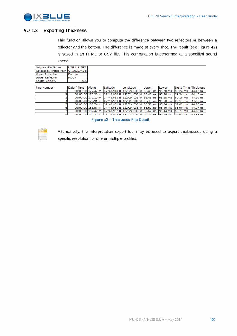
DELPH Seismic Interpretation – User Guide
V.7.1.3 Exporting Thickness
This function allows you to compute the difference between two reflectors or between a
reflector and the bottom. The difference is made at every shot. The result (see Figure 42)
is saved in an HTML or CSV file. This computation is performed at a specified sound
speed.
Figure 42 – Thickness File Detail
Alternatively, the Interpretation export tool may be used to export thicknesses using a
specific resolution for one or multiple profiles.
MU-DSI-AN-v30 Ed. A – May 2014 107
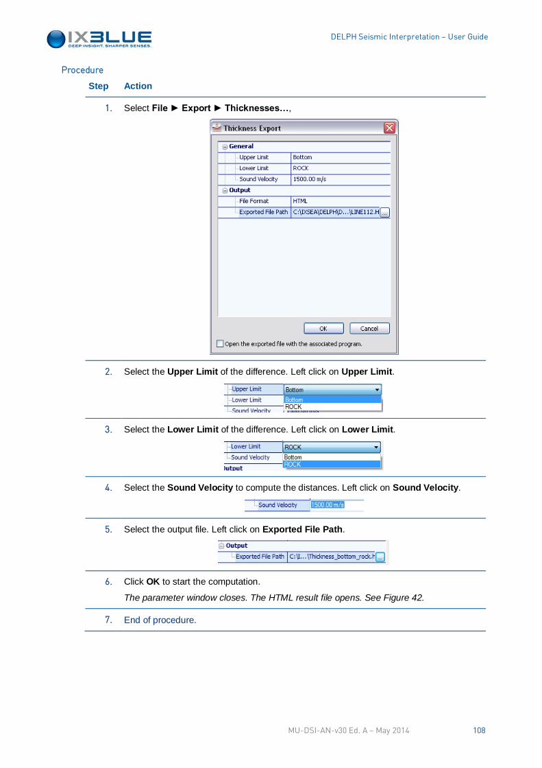
DELPH Seismic Interpretation – User Guide
Step Action
1. Select File ► Export ► Thicknesses…,
2. Select the Upper Limit of the difference. Left click on Upper Limit.
3. Select the Lower Limit of the difference. Left click on Lower Limit.
4. Select the Sound Velocity to compute the distances. Left click on Sound Velocity.
5. Select the output file. Left click on Exported File Path.
6. Click OK to start the computation.
The parameter window closes. The HTML result file opens. See Figure 42.
7. End of procedure.
Procedure
MU-DSI-AN-v30 Ed. A – May 2014 108
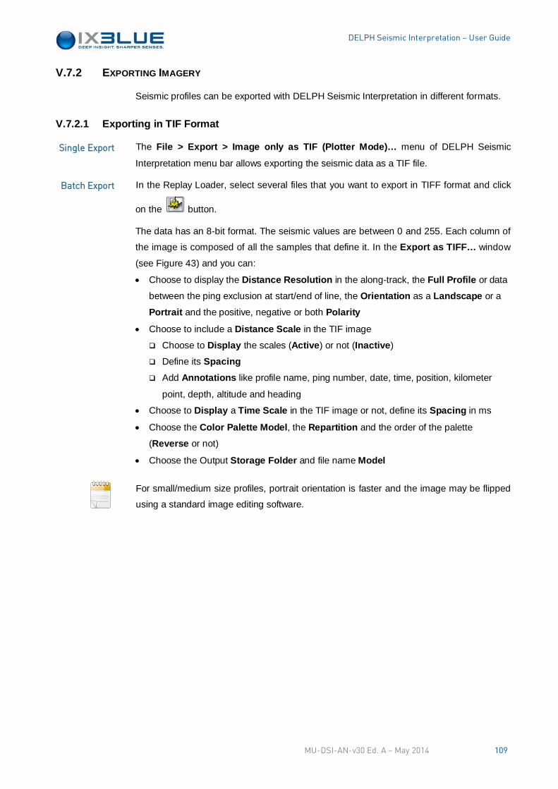
DELPH Seismic Interpretation – User Guide
V.7.2 EXPORTING IMAGERY
Seismic profiles can be exported with DELPH Seismic Interpretation in different formats.
V.7.2.1 Exporting in TIF Format
The File > Export > Image only as TIF (Plotter Mode)… menu of DELPH Seismic
Interpretation menu bar allows exporting the seismic data as a TIF file.
In the Replay Loader, select several files that you want to export in TIFF format and click
on the button.
The data has an 8-bit format. The seismic values are between 0 and 255. Each column of
the image is composed of all the samples that define it. In the Export as TIFF… window
(see Figure 43) and you can:
• Choose to display the Distance Resolution in the along-track, the Full Profile or data
between the ping exclusion at start/end of line, the Orientation as a Landscape or a
Portrait and the positive, negative or both Polarity
• Choose to include a Distance Scale in the TIF image
Choose to Display the scales (Active) or not (Inactive)
Define its Spacing
Add Annotations like profile name, ping number, date, time, position, kilometer
point, depth, altitude and heading
• Choose to Display a Time Scale in the TIF image or not, define its Spacing in ms
• Choose the Color Palette Model, the Repartition and the order of the palette
(Reverse or not)
• Choose the Output Storage Folder and file name Model
For small/medium size profiles, portrait orientation is faster and the image may be flipped
using a standard image editing software.
Single Export
Batch Export
MU-DSI-AN-v30 Ed. A – May 2014 109
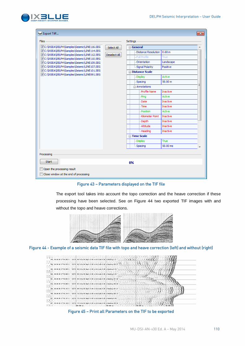
DELPH Seismic Interpretation – User Guide
Figure 43 – Parameters displayed on the TIF file
The export tool takes into account the topo correction and the heave correction if these
processing have been selected. See on Figure 44 two exported TIF images with and
without the topo and heave corrections.
Figure 44 - Example of a seismic data TIF file with topo and heave correction (left) and without (right)
Figure 45 – Print all Parameters on the TIF to be exported
MU-DSI-AN-v30 Ed. A – May 2014 110
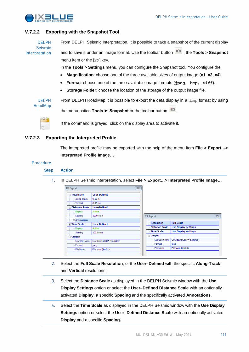
DELPH Seismic Interpretation – User Guide
V.7.2.2 Exporting with the Snapshot Tool
From DELPH Seismic Interpretation, it is possible to take a snapshot of the current display
and to save it under an image format. Use the toolbar button , the Tools > Snapshot
menu item or the [F9] key.
In the Tools > Settings menu, you can configure the Snapshot tool. You configure the
• Magnification: choose one of the three available sizes of output image (x1, x2, x4).
• Format: choose one of the three available image formats (jpeg, bmp, tiff).
• Storage Folder: choose the location of the storage of the output image file.
From DELPH RoadMap it is possible to export the data display in a .bmp format by using
the menu option Tools ► Snapshot or the toolbar button .
If the command is grayed, click on the display area to activate it.
V.7.2.3 Exporting the Interpreted Profile
The interpreted profile may be exported with the help of the menu item File > Export…> Interpreted Profile Image…
Step Action
1. In DELPH Seismic Interpretation, select File > Export…> Interpreted Profile Image…
2. Select the Full Scale Resolution, or the User–Defined with the specific Along-Track
and Vertical resolutions.
3. Select the Distance Scale as displayed in the DELPH Seismic window with the Use Display Settings option or select the User–Defined Distance Scale with an optionally
activated Display, a specific Spacing and the specifically activated Annotations.
4. Select the Time Scale as displayed in the DELPH Seismic window with the Use Display Settings option or select the User–Defined Distance Scale with an optionally activated
Display and a specific Spacing.
DELPH Seismic
Interpretation
DELPH RoadMap
Procedure
MU-DSI-AN-v30 Ed. A – May 2014 111

DELPH Seismic Interpretation – User Guide
Step Action
5. Enter the Output settings: Storage Folder, Format and File Name.
6. Click on OK to validate your choice.
The export takes place.
7. End of procedure.
MU-DSI-AN-v30 Ed. A – May 2014 112
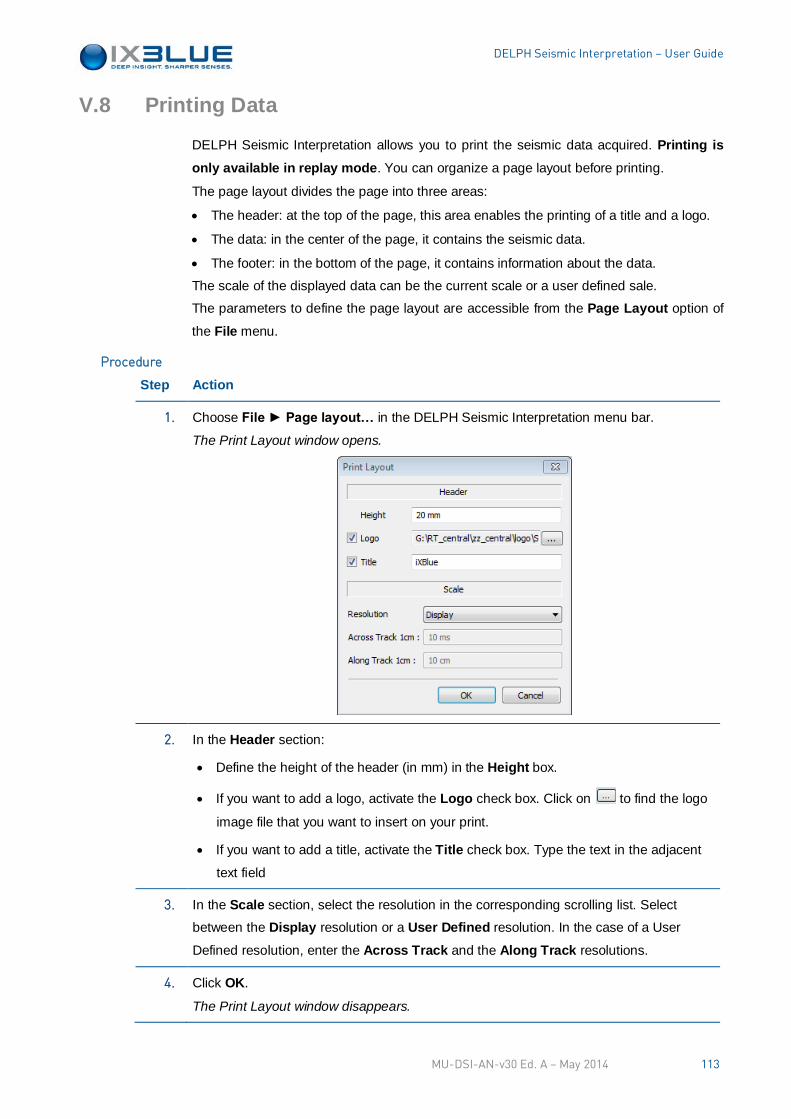
DELPH Seismic Interpretation – User Guide
V.8 Printing Data
DELPH Seismic Interpretation allows you to print the seismic data acquired. Printing is only available in replay mode. You can organize a page layout before printing.
The page layout divides the page into three areas:
• The header: at the top of the page, this area enables the printing of a title and a logo.
• The data: in the center of the page, it contains the seismic data.
• The footer: in the bottom of the page, it contains information about the data.
The scale of the displayed data can be the current scale or a user defined sale.
The parameters to define the page layout are accessible from the Page Layout option of
the File menu.
Step Action
1. Choose File ► Page layout… in the DELPH Seismic Interpretation menu bar.
The Print Layout window opens.
2. In the Header section:
• Define the height of the header (in mm) in the Height box.
• If you want to add a logo, activate the Logo check box. Click on to find the logo
image file that you want to insert on your print.
• If you want to add a title, activate the Title check box. Type the text in the adjacent
text field
3. In the Scale section, select the resolution in the corresponding scrolling list. Select
between the Display resolution or a User Defined resolution. In the case of a User
Defined resolution, enter the Across Track and the Along Track resolutions.
4. Click OK.
The Print Layout window disappears.
Procedure
MU-DSI-AN-v30 Ed. A – May 2014 113
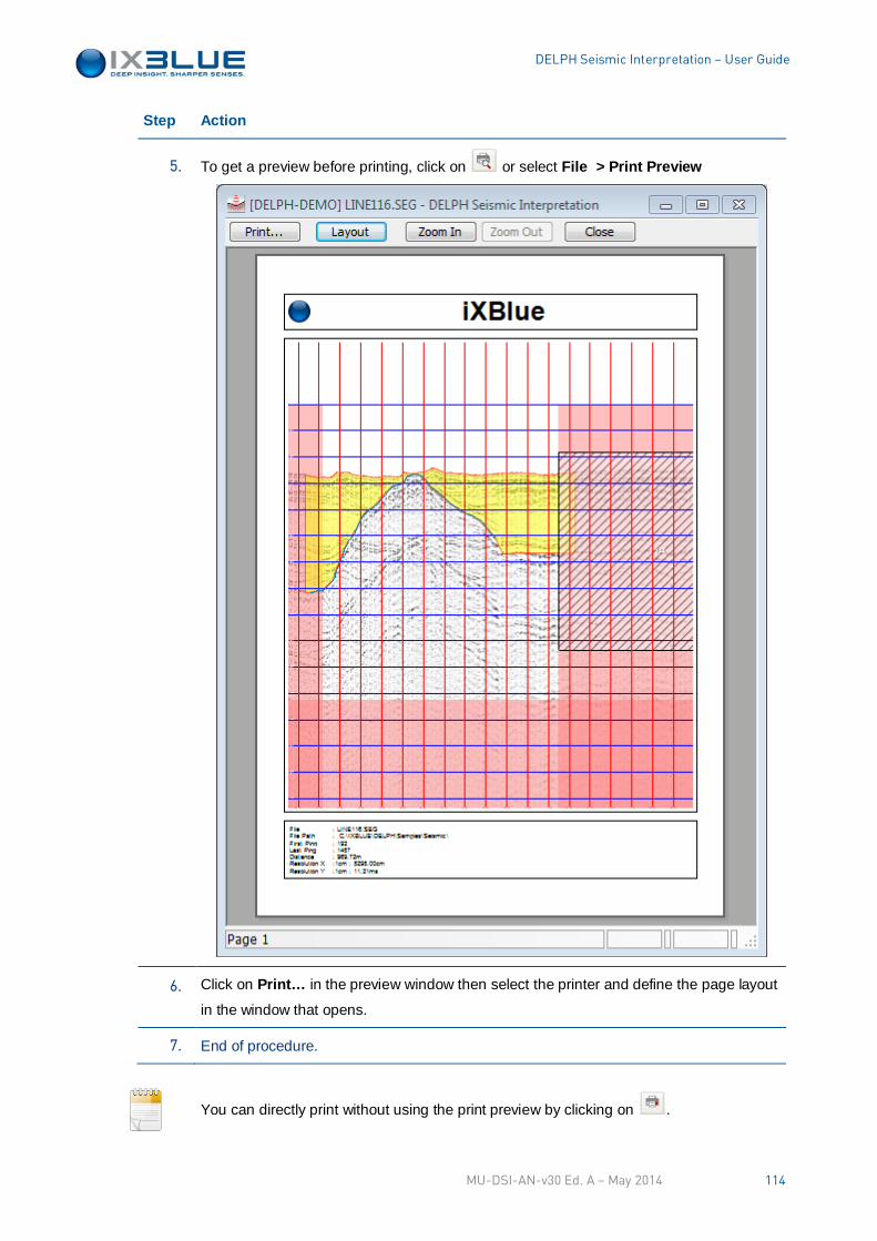
DELPH Seismic Interpretation – User Guide
Step Action
5. To get a preview before printing, click on or select File > Print Preview
6. Click on Print… in the preview window then select the printer and define the page layout
in the window that opens.
7. End of procedure.
You can directly print without using the print preview by clicking on .
MU-DSI-AN-v30 Ed. A – May 2014 114
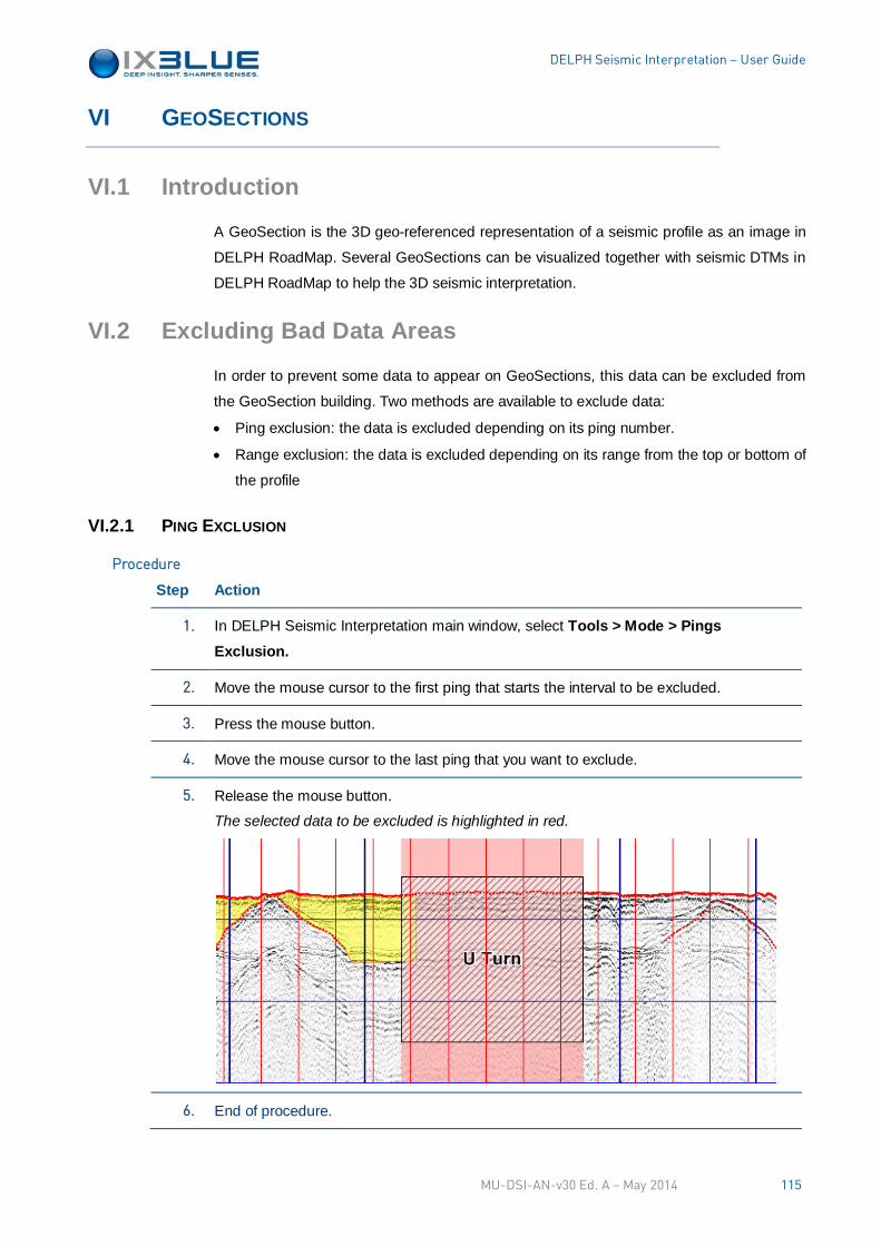
DELPH Seismic Interpretation – User Guide
VI GEOSECTIONS
VI.1 Introduction
A GeoSection is the 3D geo-referenced representation of a seismic profile as an image in
DELPH RoadMap. Several GeoSections can be visualized together with seismic DTMs in
DELPH RoadMap to help the 3D seismic interpretation.
VI.2 Excluding Bad Data Areas
In order to prevent some data to appear on GeoSections, this data can be excluded from
the GeoSection building. Two methods are available to exclude data:
• Ping exclusion: the data is excluded depending on its ping number.
• Range exclusion: the data is excluded depending on its range from the top or bottom of
the profile
VI.2.1 PING EXCLUSION
Step Action
1. In DELPH Seismic Interpretation main window, select Tools > Mode > Pings Exclusion.
2. Move the mouse cursor to the first ping that starts the interval to be excluded.
3. Press the mouse button.
4. Move the mouse cursor to the last ping that you want to exclude.
5. Release the mouse button.
The selected data to be excluded is highlighted in red.
6. End of procedure.
Procedure
MU-DSI-AN-v30 Ed. A – May 2014 115
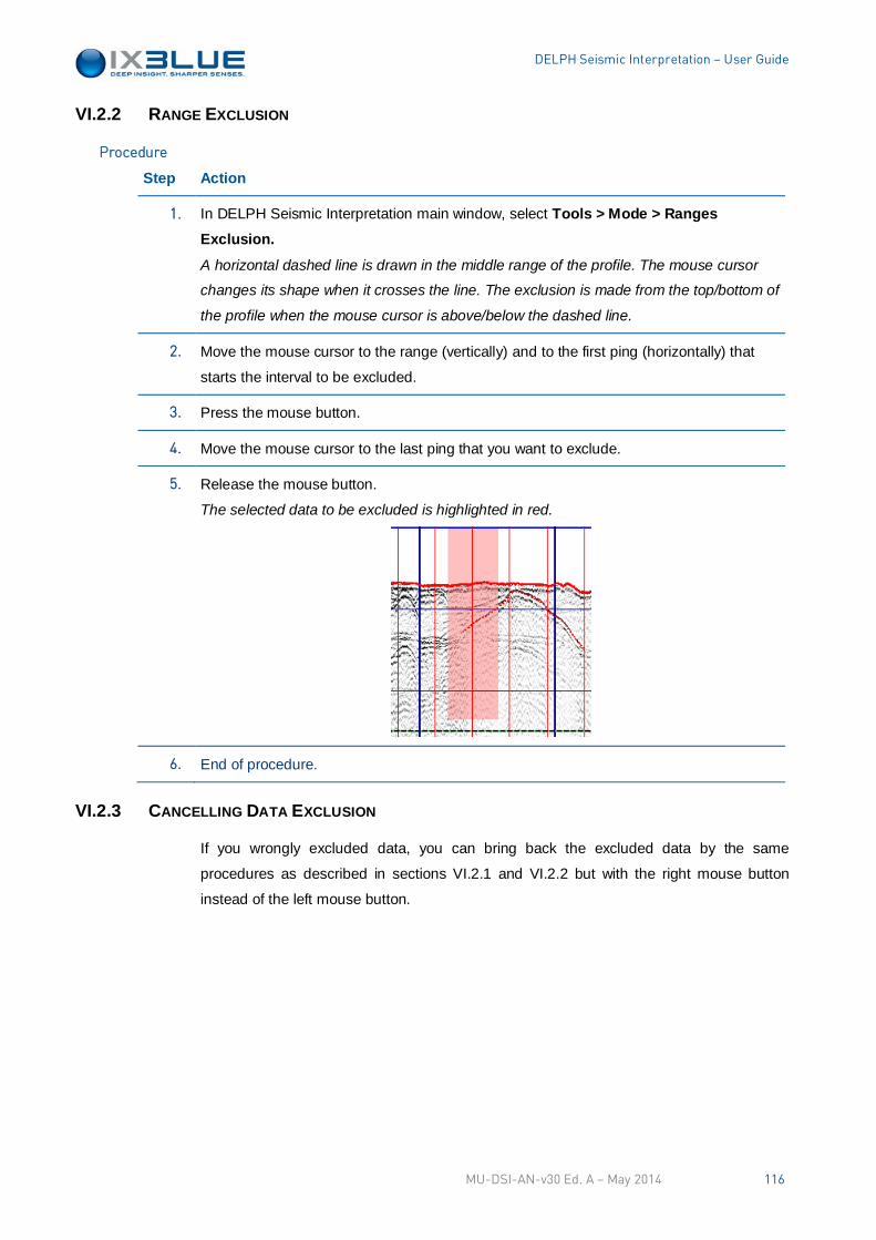
DELPH Seismic Interpretation – User Guide
VI.2.2 RANGE EXCLUSION
Step Action
1. In DELPH Seismic Interpretation main window, select Tools > Mode > Ranges Exclusion.
A horizontal dashed line is drawn in the middle range of the profile. The mouse cursor
changes its shape when it crosses the line. The exclusion is made from the top/bottom of
the profile when the mouse cursor is above/below the dashed line.
2. Move the mouse cursor to the range (vertically) and to the first ping (horizontally) that
starts the interval to be excluded.
3. Press the mouse button.
4. Move the mouse cursor to the last ping that you want to exclude.
5. Release the mouse button.
The selected data to be excluded is highlighted in red.
6. End of procedure.
VI.2.3 CANCELLING DATA EXCLUSION
If you wrongly excluded data, you can bring back the excluded data by the same
procedures as described in sections VI.2.1 and VI.2.2 but with the right mouse button
instead of the left mouse button.
Procedure
MU-DSI-AN-v30 Ed. A – May 2014 116
DELPH Seismic Interpretation – User Guide
VI.3 Building GeoSections
VI.3.1 GEOSECTION PRINCIPLE
The GeoSection image is built accordingly to the following parameters:
• Processing Parameters
Horizontal Resolution: in meters
Vertical Resolution: in propagation time
Excluded Areas: can be included or not in the geo-section.
Transparent Water-column: is an option to display or not the data acquired in the
water column.
Signal Polarity: is an option to input the Positive or Negative or both Pos&Neg
values of the trace in the geo-section.
Navigation Precision: The smooth ship navigation is decimated in segments
forming a broken line. The precision entered by the operator corresponds to the
maximum orthogonal distance between the decimated segments and the actual
navigation of the survey vessel.
• Geodesy of the Input data and of the Chart in which the GeoSections are to be
inserted.
• Color palette: including the Color Model, the Color Repartition and the eventual
inversion (Reverse).
• Output/File Name: In case of multiple GeoSections there are different ways to name
the files. A few models for multiple files are proposed. You can also define his own
model.
VI.3.2 BUILDING GEOSECTIONS IN REPLAY MODE
The GeoSection building is launched directly from the seismic file listed in DELPH Seismic
Replay Loader. Follow the procedure to build a GeoSection.
MU-DSI-AN-v30 Ed. A – May 2014 117
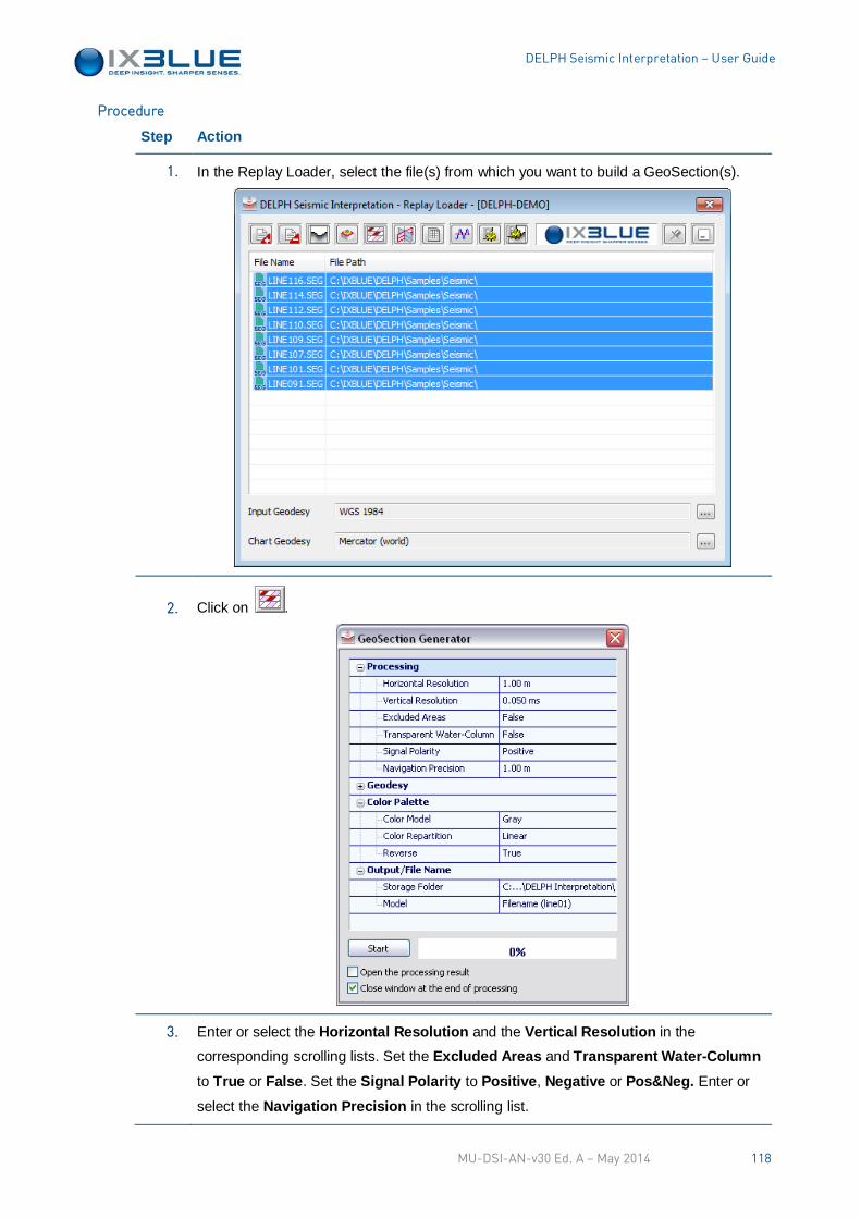
DELPH Seismic Interpretation – User Guide
Step Action
1. In the Replay Loader, select the file(s) from which you want to build a GeoSection(s).
2. Click on .
3. Enter or select the Horizontal Resolution and the Vertical Resolution in the
corresponding scrolling lists. Set the Excluded Areas and Transparent Water-Column
to True or False. Set the Signal Polarity to Positive, Negative or Pos&Neg. Enter or
select the Navigation Precision in the scrolling list.
Procedure
MU-DSI-AN-v30 Ed. A – May 2014 118
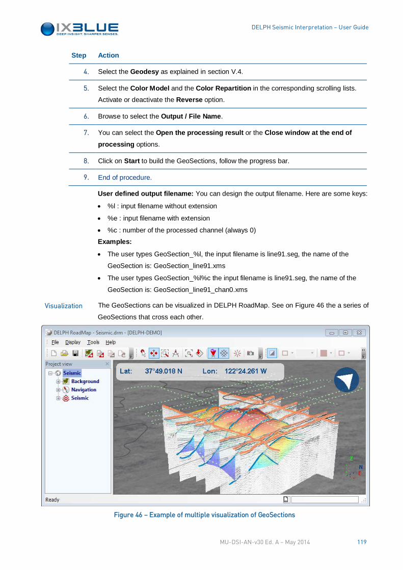
DELPH Seismic Interpretation – User Guide
Step Action
4. Select the Geodesy as explained in section V.4.
5. Select the Color Model and the Color Repartition in the corresponding scrolling lists.
Activate or deactivate the Reverse option.
6. Browse to select the Output / File Name.
7. You can select the Open the processing result or the Close window at the end of processing options.
8. Click on Start to build the GeoSections, follow the progress bar.
9. End of procedure.
User defined output filename: You can design the output filename. Here are some keys:
• %l : input filename without extension
• %e : input filename with extension
• %c : number of the processed channel (always 0)
Examples:
• The user types GeoSection_%l, the input filename is line91.seg, the name of the
GeoSection is: GeoSection_line91.xms
• The user types GeoSection_%l%c the input filename is line91.seg, the name of the
GeoSection is: GeoSection_line91_chan0.xms
The GeoSections can be visualized in DELPH RoadMap. See on Figure 46 the a series of
GeoSections that cross each other.
Figure 46 – Example of multiple visualization of GeoSections
Visualization
MU-DSI-AN-v30 Ed. A – May 2014 119
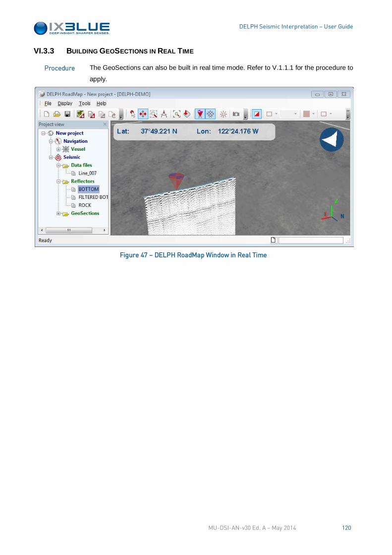
DELPH Seismic Interpretation – User Guide
VI.3.3 BUILDING GEOSECTIONS IN REAL TIME
The GeoSections can also be built in real time mode. Refer to V.1.1.1 for the procedure to
apply.
Figure 47 – DELPH RoadMap Window in Real Time
Procedure
MU-DSI-AN-v30 Ed. A – May 2014 120
DELPH Seismic Interpretation – User Guide
VII DIGITAL TERRAIN MODELING
VII.1 Introduction
DELPH Seismic offers the ability to build Digital Terrain Models (DTM) from digitized
reflectors belonging to the same geological interface and to different seismic profiles. The
DTM is first built as a Triangular Irregular Model (TIN). It is then gridded on a regular grid
with a user defined sampling. At the end the DTM is based on a regular grid.
The sea bottom digitized from seismic profiles can also be used to build a DTM. The 3D
View option in DELPH RoadMap allows multiple DTM visualization. The DTM building can
be indifferently launched from the Replay Loader or from DELPH RoadMap.
VII.2 Excluding Bad Data Areas
See section VI.2.
VII.3 Building DTMs
VII.3.1 PARAMETERS A few parameters are needed to build a reflector DTM:
• Processing parameters
Resolution: This parameter is the size of the grid cell. A high resolution leads to a
complex DTM (large number of triangles) and costs a long time to compute.
Use Exclusion Areas: This parameter let you choose if you want to include in the
DTM all the data that you excluded in the interpretation or not.
Automatic Gap Detection: This option detects the convex holes in the DTM so that
these holes are not filled during the TIN building. It is recommended in the case of
multi segment reflectors so that the space between the two segments is not
interpolated. The limits of this algorithm are the presence of non convex and islands
in the holes.
• Geodesy parameters
Input: geodesy of the input data.
Chart: geodesy of the resulting map.
• Output/File Name
Storage file: path and filename of the DTM. The DTM is stored in a .xmd file. See
Appendix A.1 for more details about this format.
• Options: You can choose to open immediately the DTM in DELPH RoadMap and to
close the DTM generator window at the end of the processing.
MU-DSI-AN-v30 Ed. A – May 2014 121
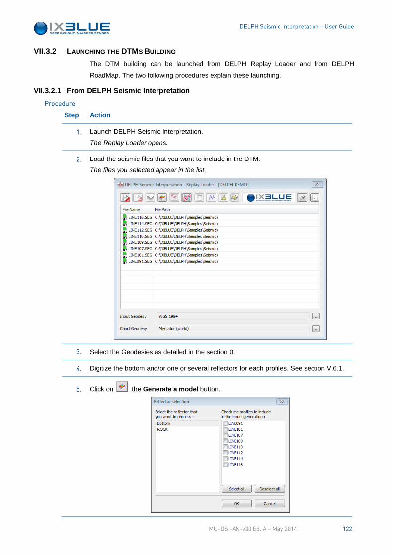
DELPH Seismic Interpretation – User Guide
VII.3.2 LAUNCHING THE DTMS BUILDING The DTM building can be launched from DELPH Replay Loader and from DELPH
RoadMap. The two following procedures explain these launching.
VII.3.2.1 From DELPH Seismic Interpretation
Step Action
1. Launch DELPH Seismic Interpretation.
The Replay Loader opens.
2. Load the seismic files that you want to include in the DTM.
The files you selected appear in the list.
3. Select the Geodesies as detailed in the section 0.
4. Digitize the bottom and/or one or several reflectors for each profiles. See section V.6.1.
5. Click on , the Generate a model button.
Procedure
MU-DSI-AN-v30 Ed. A – May 2014 122
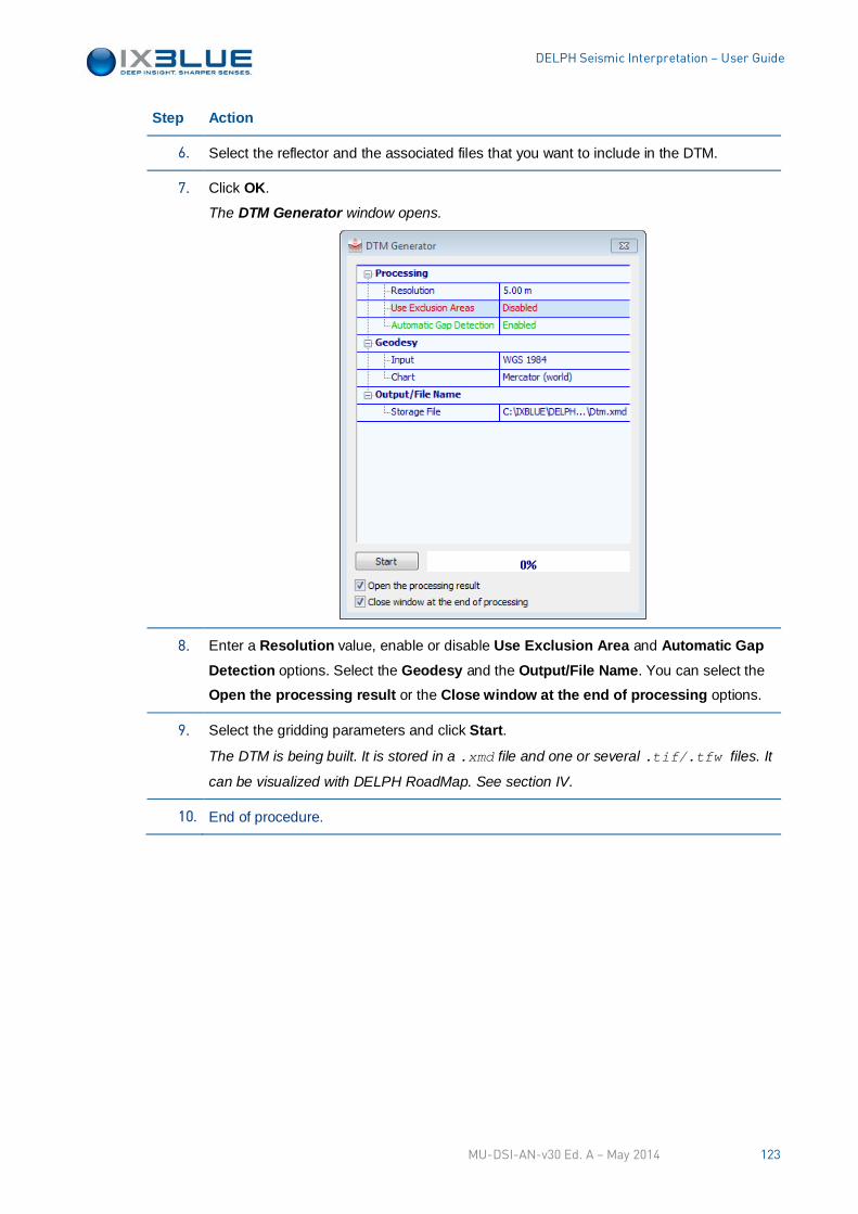
DELPH Seismic Interpretation – User Guide
Step Action
6. Select the reflector and the associated files that you want to include in the DTM.
7. Click OK.
The DTM Generator window opens.
8. Enter a Resolution value, enable or disable Use Exclusion Area and Automatic Gap Detection options. Select the Geodesy and the Output/File Name. You can select the
Open the processing result or the Close window at the end of processing options.
9. Select the gridding parameters and click Start.
The DTM is being built. It is stored in a .xmd file and one or several .tif/.tfw files. It
can be visualized with DELPH RoadMap. See section IV.
10. End of procedure.
MU-DSI-AN-v30 Ed. A – May 2014 123
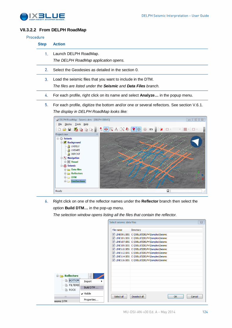
DELPH Seismic Interpretation – User Guide
VII.3.2.2 From DELPH RoadMap
Step Action
1. Launch DELPH RoadMap.
The DELPH RoadMap application opens.
2. Select the Geodesies as detailed in the section 0.
3. Load the seismic files that you want to include in the DTM.
The files are listed under the Seismic and Data Files branch.
4. For each profile, right click on its name and select Analyze… in the popup menu.
5. For each profile, digitize the bottom and/or one or several reflectors. See section V.6.1.
The display in DELPH RoadMap looks like:
6. Right click on one of the reflector names under the Reflector branch then select the
option Build DTM… in the pop-up menu.
The selection window opens listing all the files that contain the reflector.
Procedure
MU-DSI-AN-v30 Ed. A – May 2014 124
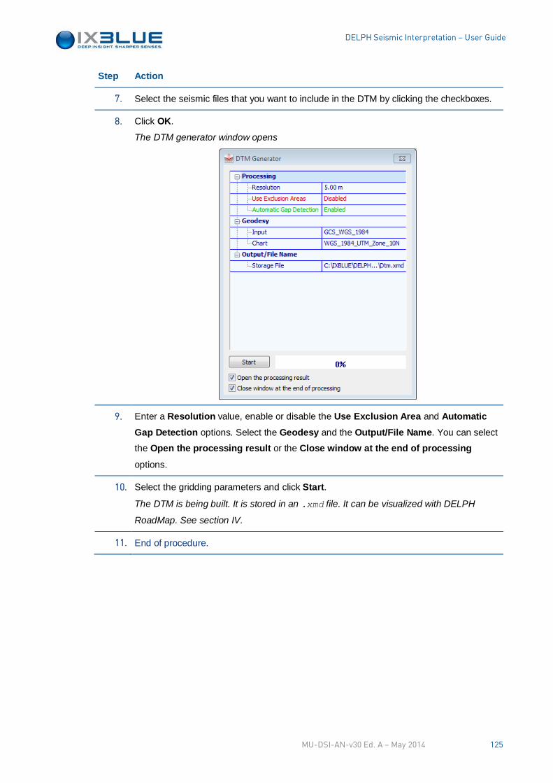
DELPH Seismic Interpretation – User Guide
Step Action
7. Select the seismic files that you want to include in the DTM by clicking the checkboxes.
8. Click OK.
The DTM generator window opens
9. Enter a Resolution value, enable or disable the Use Exclusion Area and Automatic Gap Detection options. Select the Geodesy and the Output/File Name. You can select
the Open the processing result or the Close window at the end of processing
options.
10. Select the gridding parameters and click Start.
The DTM is being built. It is stored in an .xmd file. It can be visualized with DELPH
RoadMap. See section IV.
11. End of procedure.
MU-DSI-AN-v30 Ed. A – May 2014 125
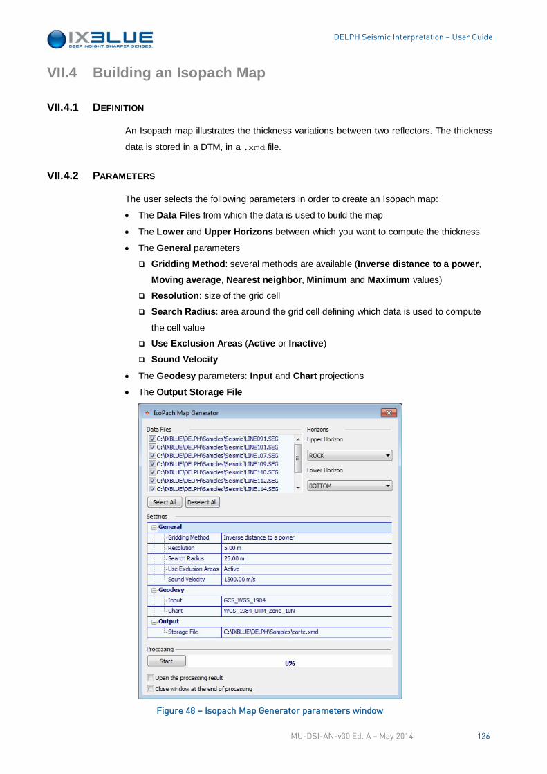
DELPH Seismic Interpretation – User Guide
VII.4 Building an Isopach Map
VII.4.1 DEFINITION
An Isopach map illustrates the thickness variations between two reflectors. The thickness
data is stored in a DTM, in a .xmd file.
VII.4.2 PARAMETERS
The user selects the following parameters in order to create an Isopach map:
• The Data Files from which the data is used to build the map
• The Lower and Upper Horizons between which you want to compute the thickness
• The General parameters
Gridding Method: several methods are available (Inverse distance to a power, Moving average, Nearest neighbor, Minimum and Maximum values)
Resolution: size of the grid cell
Search Radius: area around the grid cell defining which data is used to compute
the cell value Use Exclusion Areas (Active or Inactive)
Sound Velocity
• The Geodesy parameters: Input and Chart projections
• The Output Storage File
Figure 48 – Isopach Map Generator parameters window
MU-DSI-AN-v30 Ed. A – May 2014 126
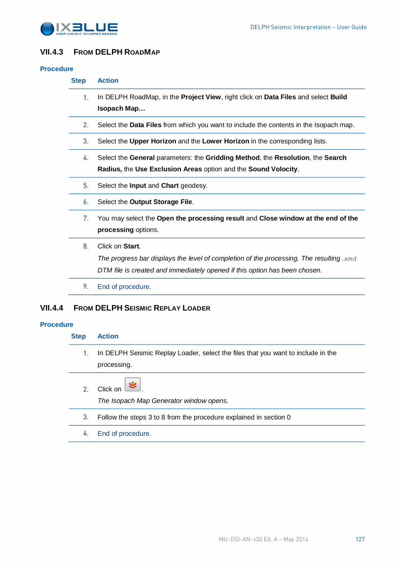
DELPH Seismic Interpretation – User Guide
VII.4.3 FROM DELPH ROADMAP
Procedure Step Action
1. In DELPH RoadMap, in the Project View, right click on Data Files and select Build Isopach Map…
2. Select the Data Files from which you want to include the contents in the Isopach map.
3. Select the Upper Horizon and the Lower Horizon in the corresponding lists.
4. Select the General parameters: the Gridding Method, the Resolution, the Search Radius, the Use Exclusion Areas option and the Sound Volocity.
5. Select the Input and Chart geodesy.
6. Select the Output Storage File.
7. You may select the Open the processing result and Close window at the end of the processing options.
8. Click on Start.
The progress bar displays the level of completion of the processing. The resulting .xmd
DTM file is created and immediately opened if this option has been chosen.
9. End of procedure.
VII.4.4 FROM DELPH SEISMIC REPLAY LOADER
Procedure Step Action
1. In DELPH Seismic Replay Loader, select the files that you want to include in the
processing.
2. Click on .
The Isopach Map Generator window opens.
3. Follow the steps 3 to 8 from the procedure explained in section 0
4. End of procedure.
MU-DSI-AN-v30 Ed. A – May 2014 127
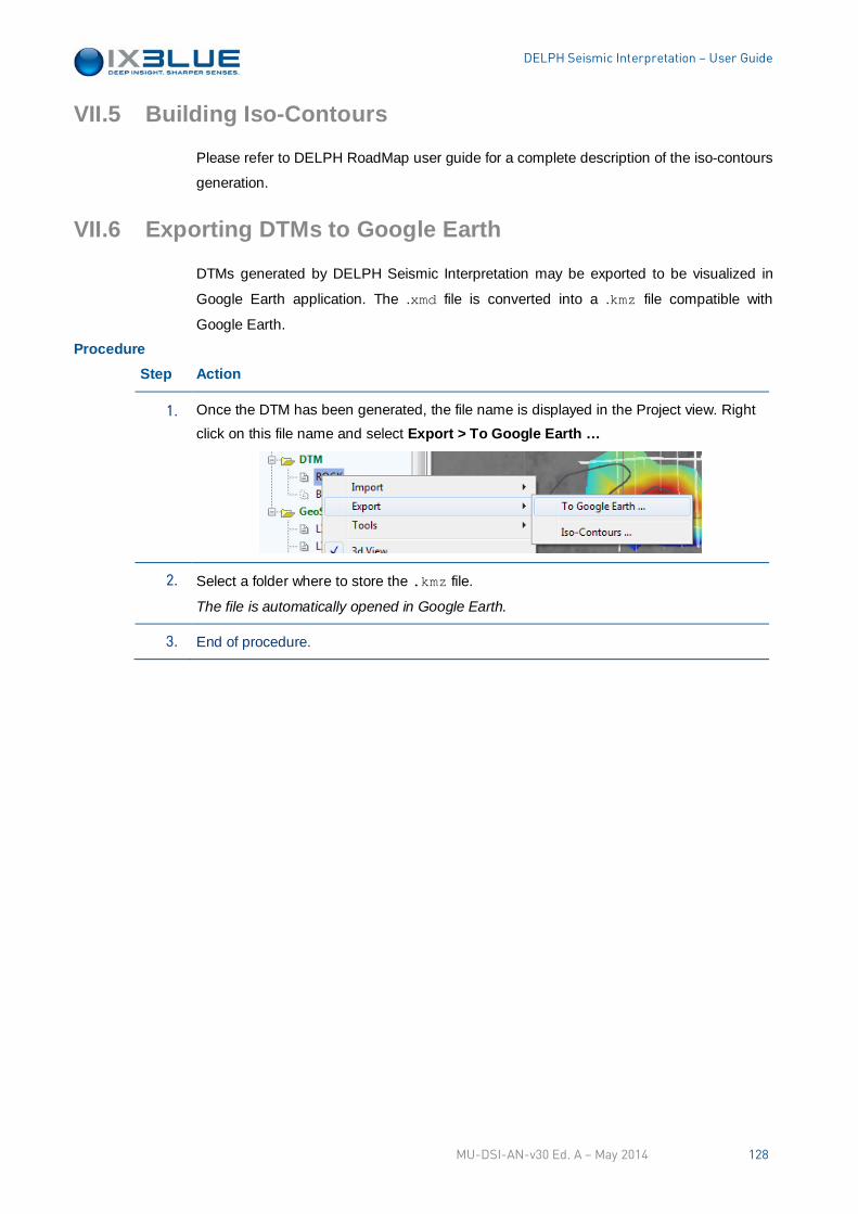
DELPH Seismic Interpretation – User Guide
VII.5 Building Iso-Contours
Please refer to DELPH RoadMap user guide for a complete description of the iso-contours
generation.
VII.6 Exporting DTMs to Google Earth
DTMs generated by DELPH Seismic Interpretation may be exported to be visualized in
Google Earth application. The .xmd file is converted into a .kmz file compatible with
Google Earth.
Procedure Step Action
1. Once the DTM has been generated, the file name is displayed in the Project view. Right click on this file name and select Export > To Google Earth …
2. Select a folder where to store the .kmz file.
The file is automatically opened in Google Earth.
3. End of procedure.
MU-DSI-AN-v30 Ed. A – May 2014 128
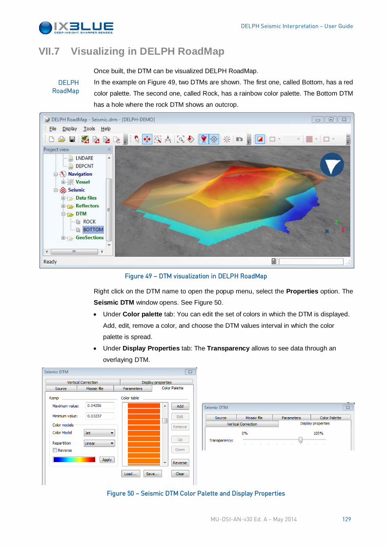
DELPH Seismic Interpretation – User Guide
VII.7 Visualizing in DELPH RoadMap
Once built, the DTM can be visualized DELPH RoadMap.
In the example on Figure 49, two DTMs are shown. The first one, called Bottom, has a red
color palette. The second one, called Rock, has a rainbow color palette. The Bottom DTM
has a hole where the rock DTM shows an outcrop.
Figure 49 – DTM visualization in DELPH RoadMap
Right click on the DTM name to open the popup menu, select the Properties option. The
Seismic DTM window opens. See Figure 50.
• Under Color palette tab: You can edit the set of colors in which the DTM is displayed.
Add, edit, remove a color, and choose the DTM values interval in which the color
palette is spread.
• Under Display Properties tab: The Transparency allows to see data through an
overlaying DTM.
Figure 50 – Seismic DTM Color Palette and Display Properties
DELPH RoadMap
MU-DSI-AN-v30 Ed. A – May 2014 129

DELPH Seismic Interpretation – User Guide
iXBlue CONTACT - SUPPORT 24/7 CUSTOMER SUPPORT HELPLINE
FOR NON-EMERGENCY SUPPORT:
FOR GENUINE EMERGENCIES ONLY:
North America / NORAM +1 888-600-7573 Extension 2
Europe Middle-East Africa Latin-America / EMEA-LATAM +33 1 30 08 98 98 Asia Pacific / APAC +65 6747 7027
MU-DSI-AN-v30 Ed. A – May 2014 130
DELPH Seismic Interpretation – User Guide
iXBlue CONTACT - SALES
North America / NORAM +1 888-600-7573 iXBlue Inc Boston US 11 Erie Drive, Natick, MA 01760, United States Office: Houston, USA
Europe Middle-East Africa Latin-America / EMEA-LATAM +33 1 30 08 88 88 iXBlue SAS Marly France 52 avenue de l’Europe Marly le Roi, 78160, France Offices: Dubai, Germany, Netherlands, Norway, UK, Italy
Asia Pacific / APAC +65 6747 4912 iXBlue Pte Limited Singapore 15A Changi Business Park Central 1#04-02 Eightrium Singapore 486035 Offices: Australia, China, India
MU-DSI-AN-v30 Ed. A – May 2014 131
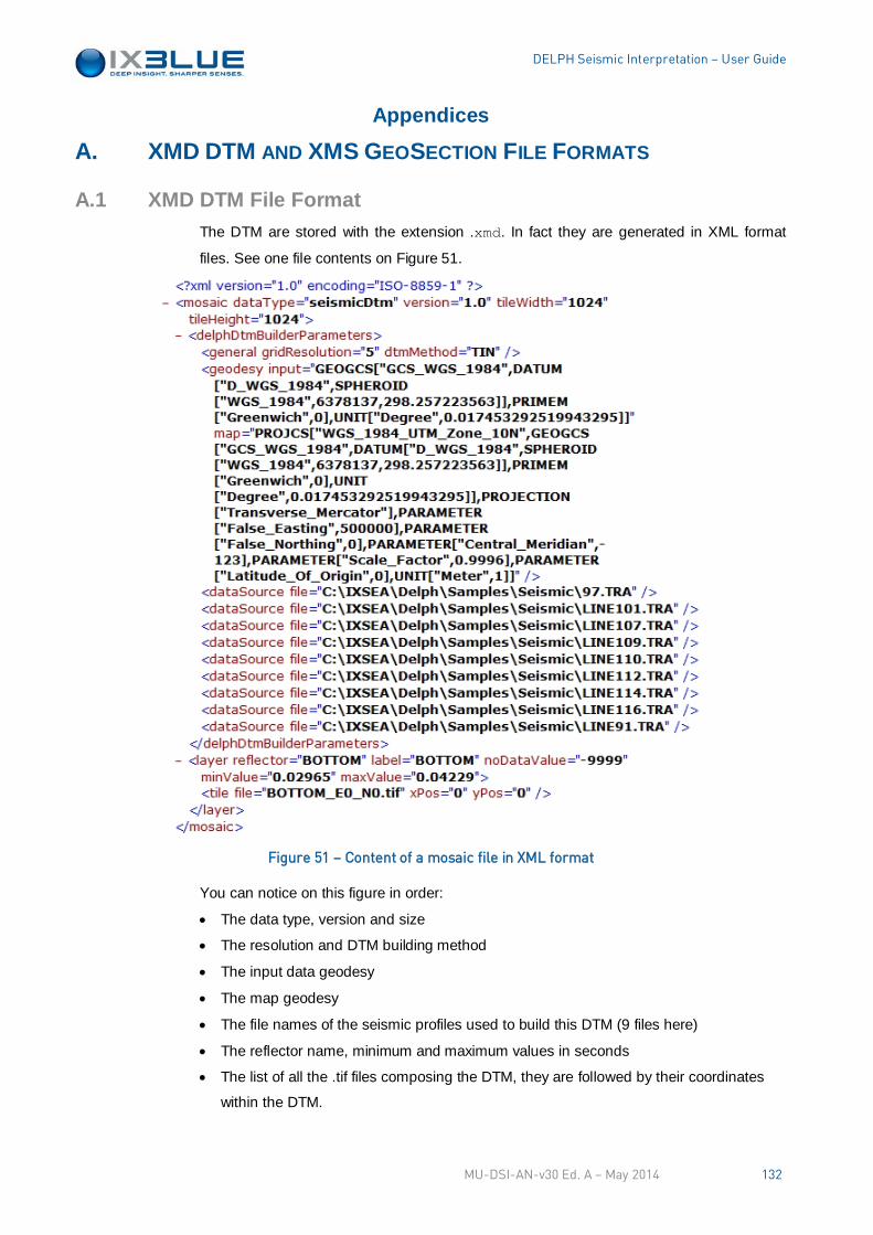
DELPH Seismic Interpretation – User Guide
Appendices
A. XMD DTM AND XMS GEOSECTION FILE FORMATS
A.1 XMD DTM File Format The DTM are stored with the extension .xmd. In fact they are generated in XML format
files. See one file contents on Figure 51.
Figure 51 – Content of a mosaic file in XML format
You can notice on this figure in order:
• The data type, version and size
• The resolution and DTM building method
• The input data geodesy
• The map geodesy
• The file names of the seismic profiles used to build this DTM (9 files here)
• The reflector name, minimum and maximum values in seconds
• The list of all the .tif files composing the DTM, they are followed by their coordinates
within the DTM.
MU-DSI-AN-v30 Ed. A – May 2014 132
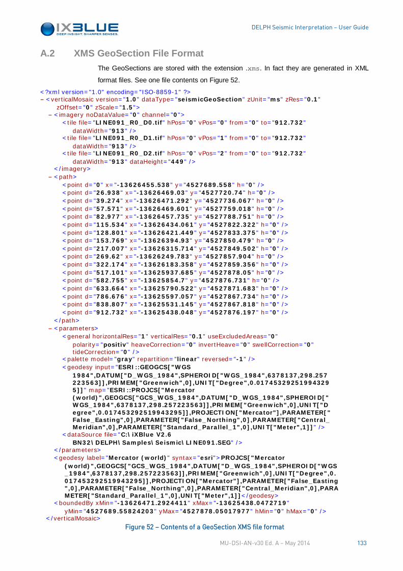
DELPH Seismic Interpretation – User Guide
A.2 XMS GeoSection File Format The GeoSections are stored with the extension .xms. In fact they are generated in XML
format files. See one file contents on Figure 52.
<?xml version="1.0" encoding="ISO-8859-1" ?> - <verticalMosaic version="1.0" dataType="seismicGeoSection" zUnit="ms" zRes="0.1"
zOffset="0" zScale="1.5"> - <imagery noDataValue="0" channel="0">
<tile file="LINE091_R0_D0.tif" hPos="0" vPos="0" from="0" to="912.732" dataWidth="913" />
<tile file="LINE091_R0_D1.tif" hPos="0" vPos="1" from="0" to="912.732" dataWidth="913" />
<tile file="LINE091_R0_D2.tif" hPos="0" vPos="2" from="0" to="912.732" dataWidth="913" dataHeight="449" />
</imagery> - <path>
<point d="0" x="-13626455.538" y="4527689.558" h="0" /> <point d="26.938" x="-13626469.03" y="4527720.74" h="0" /> <point d="39.274" x="-13626471.292" y="4527736.067" h="0" /> <point d="57.571" x="-13626469.601" y="4527759.018" h="0" /> <point d="82.977" x="-13626457.735" y="4527788.751" h="0" /> <point d="115.534" x="-13626434.061" y="4527822.322" h="0" /> <point d="128.801" x="-13626421.449" y="4527833.375" h="0" /> <point d="153.769" x="-13626394.93" y="4527850.479" h="0" /> <point d="217.007" x="-13626315.714" y="4527849.502" h="0" /> <point d="269.62" x="-13626249.783" y="4527857.904" h="0" /> <point d="322.174" x="-13626183.358" y="4527859.356" h="0" /> <point d="517.101" x="-13625937.685" y="4527878.05" h="0" /> <point d="582.755" x="-13625854.7" y="4527876.731" h="0" /> <point d="633.664" x="-13625790.522" y="4527871.683" h="0" /> <point d="786.676" x="-13625597.057" y="4527867.734" h="0" /> <point d="838.807" x="-13625531.145" y="4527867.818" h="0" /> <point d="912.732" x="-13625438.048" y="4527876.197" h="0" />
</path> - <parameters>
<general horizontalRes="1" verticalRes="0.1" useExcludedAreas="0" polarity="positiv" heaveCorrection="0" invertHeave="0" swellCorrection="0" tideCorrection="0" />
<palette model="gray" repartition="linear" reversed="-1" /> <geodesy input="ESRI::GEOGCS["WGS
1984",DATUM["D_WGS_1984",SPHEROID["WGS_1984",6378137,298.257223563]],PRIMEM["Greenwich",0],UNIT["Degree",0.017453292519943295]]" map="ESRI::PROJCS["Mercator (world)",GEOGCS["GCS_WGS_1984",DATUM["D_WGS_1984",SPHEROID["WGS_1984",6378137,298.257223563]],PRIMEM["Greenwich",0],UNIT["Degree",0.017453292519943295]],PROJECTION["Mercator"],PARAMETER["False_Easting",0],PARAMETER["False_Northing",0],PARAMETER["Central_Meridian",0],PARAMETER["Standard_Parallel_1",0],UNIT["Meter",1]]" />
<dataSource file="C:\iXBlue V2.6 BN32\DELPH\Samples\Seismic\LINE091.SEG" />
</parameters> <geodesy label="Mercator (world)" syntax="esri">PROJCS["Mercator
(world)",GEOGCS["GCS_WGS_1984",DATUM["D_WGS_1984",SPHEROID["WGS_1984",6378137,298.257223563]],PRIMEM["Greenwich",0],UNIT["Degree",0.017453292519943295]],PROJECTION["Mercator"],PARAMETER["False_Easting",0],PARAMETER["False_Northing",0],PARAMETER["Central_Meridian",0],PARAMETER["Standard_Parallel_1",0],UNIT["Meter",1]]</geodesy>
<boundedBy xMin="-13626471.2924411" xMax="-13625438.0472719" yMin="4527689.55824203" yMax="4527878.05017977" hMin="0" hMax="0" />
</verticalMosaic> Figure 52 – Contents of a GeoSection XMS file format
MU-DSI-AN-v30 Ed. A – May 2014 133
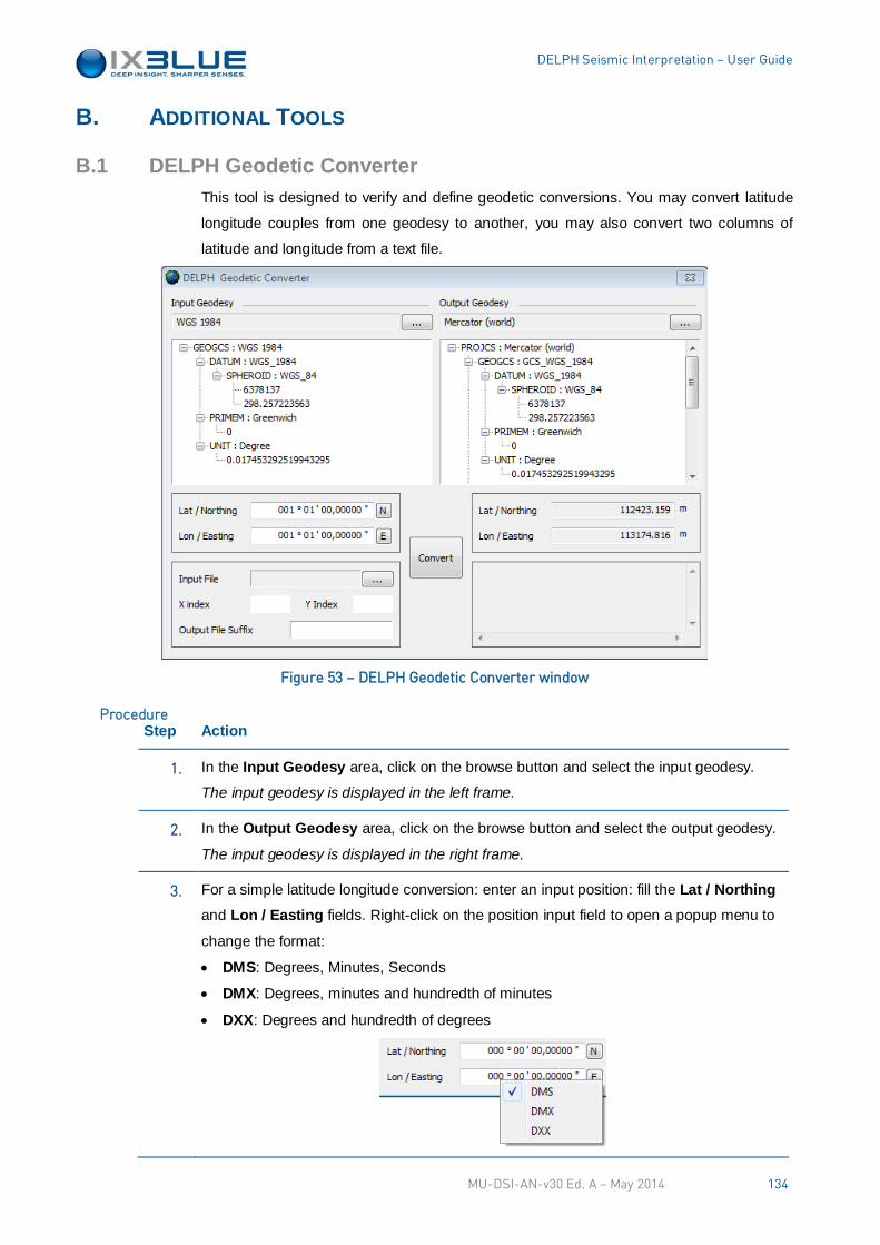
DELPH Seismic Interpretation – User Guide
B. ADDITIONAL TOOLS
B.1 DELPH Geodetic Converter This tool is designed to verify and define geodetic conversions. You may convert latitude
longitude couples from one geodesy to another, you may also convert two columns of
latitude and longitude from a text file.
Figure 53 – DELPH Geodetic Converter window
Step Action
1. In the Input Geodesy area, click on the browse button and select the input geodesy.
The input geodesy is displayed in the left frame.
2. In the Output Geodesy area, click on the browse button and select the output geodesy.
The input geodesy is displayed in the right frame.
3. For a simple latitude longitude conversion: enter an input position: fill the Lat / Northing
and Lon / Easting fields. Right-click on the position input field to open a popup menu to
change the format:
• DMS: Degrees, Minutes, Seconds
• DMX: Degrees, minutes and hundredth of minutes
• DXX: Degrees and hundredth of degrees
Procedure
MU-DSI-AN-v30 Ed. A – May 2014 134
DELPH Seismic Interpretation – User Guide
Step Action
4. For a conversion of two rows of latitude longitude from a text file: enter a text file in the Input File field. Enter the index of the latitude and longitude columns in the file into the X Index and Y Index fields. You may enter an Output File Suffix for the output file.
5. Click on Convert to perform a coordinate conversion to the output geodetic system.
The output position fields show the converted values.
6. End of procedure.
Modifications that are made on geodetic systems from this utility are available from any
other geodesy selection interface throughout DELPH software. Loading a file is possible.
MU-DSI-AN-v30 Ed. A – May 2014 135
DELPH Seismic Interpretation – User Guide
B.2 DELPH Nav Inverter This tool is designed to invert the sign of the Longitude/Easting and/or the
Latitude/Northing in a XTF file. It is a command tool.
Figure 54 – DELPH Nav Inverter Icon
Command: DELPHNavInverter [-out output] [-force true | false] [-invertX
true | false] [-invertX true | false]
Options:
• out: Path for the file to create. It can be a full file path or a file name. If not specified,
the input file with a ‘-inv’ suffix
• force: if set to true, an existing output file will be overwritten. Otherwise the processing
will be skipped. This option default is true • invertX: Change the sign for the Easting/Latitude
• invertY: Change the sign for the Northing/Longitude
Step Action
1. Open the command prompt of your operating system.
2. Type the command with the appropriate options and the path of the file to process.
3. Press [Enter]and wait until the end of the processing.
4. End of procedure.
The operator can also invert the navigation of a file by dragging the file on top of the
DELPH Nav Inverter application icon. The default options present in the .ini file are then
applied. Editing of the .ini file is possible.
Procedure
MU-DSI-AN-v30 Ed. A – May 2014 136
DELPH Seismic Interpretation – User Guide
B.3 DELPH Nav Extractor This tool allows the extraction of the navigation data present in a XTF file.
Figure 55 – DELPH Nav Extractor Icon
Command: DELPHNavExtractor [-out output][-force true|false][-format
NAV|CSV|SCSV][-header true|false][-from ship|sensor] +speed
+heading +pitch +roll +yaw +heave +depth +altitude +layback +cable
+all
• out: path for the file to create. It can be a full file path or a file name. If not specified,
the input file with a ‘-inv’ suffix.
• force: if set to true, an existing output file will be overwritten. Otherwise the processing
will be skipped, the default value is true.
• format: if set to NAV the file is a tab separated ASCII file with a .nav extension, if set
to CSV the file is a comma separated ASCII file with a .csv extension, if set to SCSV
the file is a semi-column separated ASCII file with a .scsv extension, the default value
is NAV.
• header: if set to true, a column header is added, the default value is false.
• from: defines the positioning source: if set to ship the ship position heading speed
depth are exported, if set to sensor the sensor position heading speed depth are
exported, the default value is sensor and applies only to XTF data files.
• +speed output of the ship/sensor speed data (knots)
• +heading output of the speed/sensor heading data (degrees)
• +pitch output of the sensor pitch data (degrees)
• +roll output of the sensor roll data (degrees)
• +yaw output of the sensor yaw data (degrees)
• +heave output of the sensor heave data (meters)
• +depth output of the sensor/depth depth data (meters)
• +altitude output of the sensor altitude data (meters)
• +layback output of the layback (meters)
• +cable output of the cable length value (meters)
• +kp output of the KP value
• +all output of all the above additional field data
MU-DSI-AN-v30 Ed. A – May 2014 137
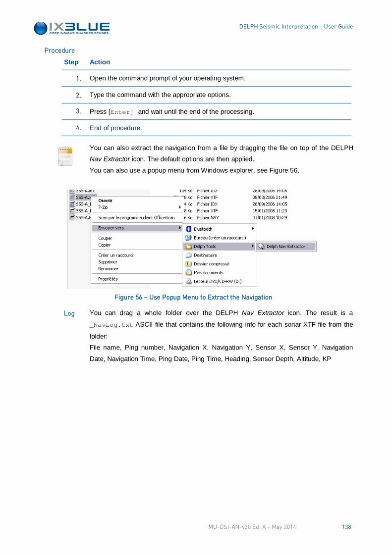
DELPH Seismic Interpretation – User Guide
Step Action
1. Open the command prompt of your operating system.
2. Type the command with the appropriate options.
3. Press [Enter] and wait until the end of the processing.
4. End of procedure.
You can also extract the navigation from a file by dragging the file on top of the DELPH
Nav Extractor icon. The default options are then applied.
You can also use a popup menu from Windows explorer, see Figure 56.
Figure 56 – Use Popup Menu to Extract the Navigation
You can drag a whole folder over the DELPH Nav Extractor icon. The result is a
_NavLog.txt ASCII file that contains the following info for each sonar XTF file from the
folder:
File name, Ping number, Navigation X, Navigation Y, Sensor X, Sensor Y, Navigation
Date, Navigation Time, Ping Date, Ping Time, Heading, Sensor Depth, Altitude, KP
Procedure
Log
MU-DSI-AN-v30 Ed. A – May 2014 138
DELPH Seismic Interpretation – User Guide
B.4 DELPH Nav Inserter - Time
The DELPH Nav Inserter - Time tool is used to merge a navigation dataset with a
geophysical dataset (sonar, seismic and magnetism). The tool provides every time
stamped data with geographic coordinates. In order to achieve this, the navigation text
data file is parsed and then interpolated to be synchronized with the geophysical dataset.
See DELPH Navigation Inserter – Time window on Figure 57.
The navigation can be imported in two different modes:
• Vessel Position: Offsets & Cable Layout are preserved and used to compute the
sensor navigation
• Sensor Position: Offsets & Cable Layout are reset and the positions come from the
sensor
A number of fields are mandatory to synchronize the Navigation File data with the pings:
• Lines to skip
• Field Separator
• Position Fields (Projected or Geographic)
• Date Field (Y/M/D)
• Time Field H:M:S.SSS
Some more optional data can be imported in the navigation insertion process:
• KP: Kilometer Point distances
• Water Depth (m): Corresponds to the complete water colum and can be gathered from
single or multi-beam sensor data
• Sensor Depth (m): Corresponds to the immersion depth of the sensor and is
commonly provided by a pressure sensor.
• Sensor Altitude (m): The altitude of the sensor above the seabed.
• Sensor Heading (°): The heading that is measured on the sensor.
• Sound Velocity (m/s): New values for the sound velocity in the water can be manually
specified or imported from the navigation file.
The synchronization between the navigation and the pings is based on the date and time
information. The ping time is commonly using the PC clock time that is synchronized to
the navigation clock time (ex: GPS time). A number of Processing options allow the fine
tuning of this synchronization to overcome most issues:
• The Import Navigation as can be set to the two possible modes Vessel Position and
Sensor Position.
• The Synchronization Mode can be set to
Timetags (XTF Only): XTF files contain an additional high resolution time tag,
based on the internal acquisition PC clock time. This data is available for both the
navigation and the pings, providing them with a common time reference basis. As
some 3rd party acquisition software do not use these fields, the time tag values
consistency must be verified using DELPH Nav Extractor utility.
MU-DSI-AN-v30 Ed. A – May 2014 139
DELPH Seismic Interpretation – User Guide
Date & Time: the Time Offset to navigation time can be defined to re-adjust the
ping time to the navigation time:
- Hours: Allows an easy correction between GMT zones
- Seconds: Allows the compensation for latency between the navigation data and
the ping time.
DELPH Nav Inserter cancels the processing when the navigation data does not
completely overlap the data files time span. This protection can be turned off by
unchecking the Strict Time Span Check option. Then, any ping which time cannot be
found in the navigation data keeps its original position. Care must be taken to ensure that
the resulting navigation remains consistent. Particularly, this must not be used when
changing the navigation data type between projected and geographic coordinates.
The output from DELPH Nav Inserter is a new set of XTF or SEGY data files that contains
the corrected navigation.
When a data file has been already processed, its processed navigation is updated with the
imported data (raw file remains unchanged). Otherwise, a new set of XTF or SEGY data
files with the corrected navigation is produced.
MU-DSI-AN-v30 Ed. A – May 2014 140
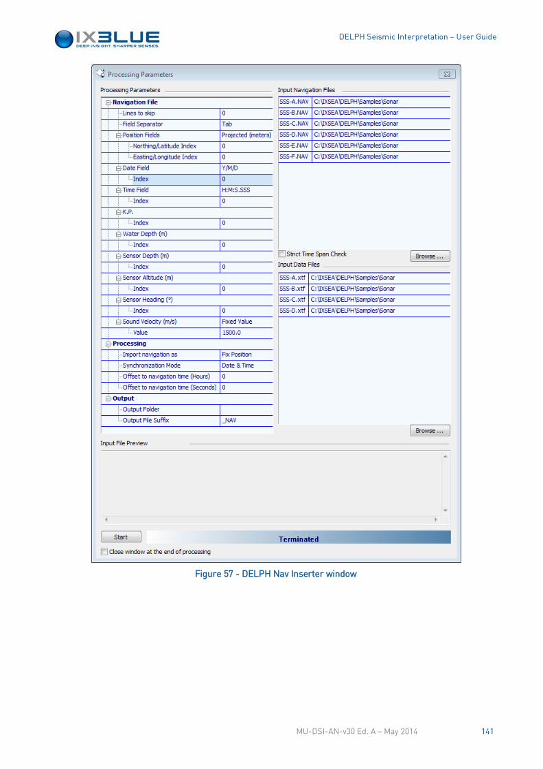
DELPH Seismic Interpretation – User Guide
Figure 57 - DELPH Nav Inserter window
MU-DSI-AN-v30 Ed. A – May 2014 141
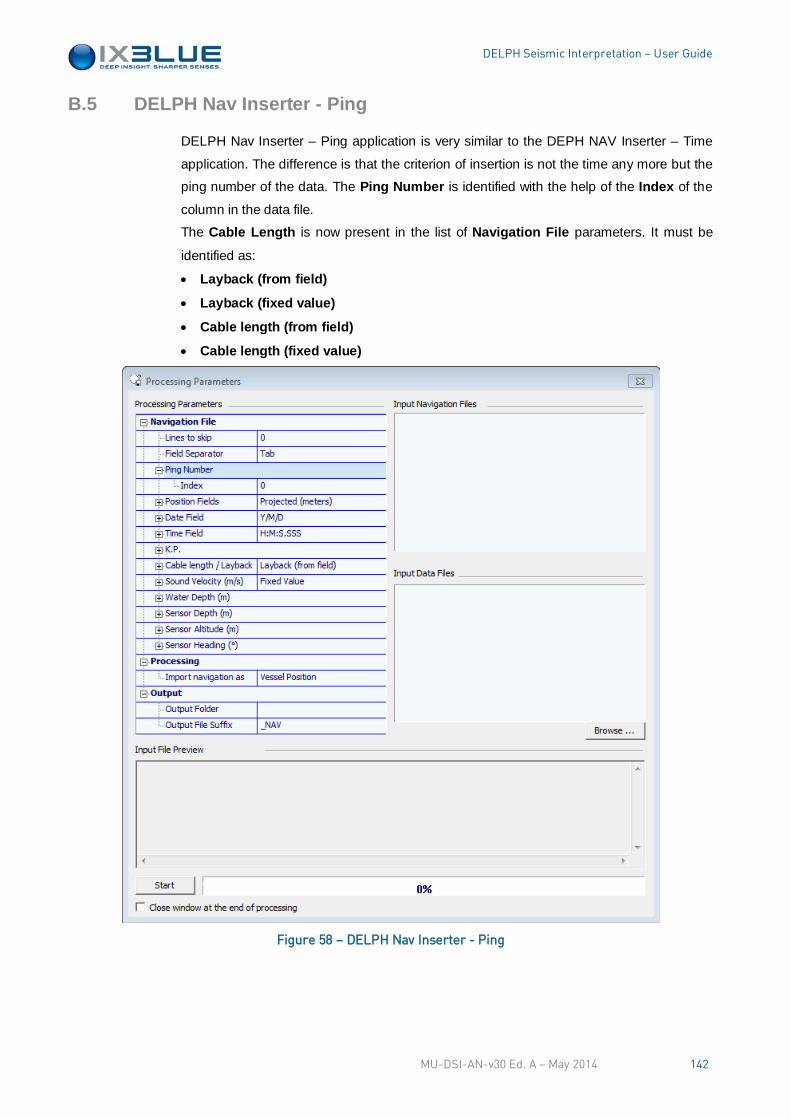
DELPH Seismic Interpretation – User Guide
B.5 DELPH Nav Inserter - Ping
DELPH Nav Inserter – Ping application is very similar to the DEPH NAV Inserter – Time
application. The difference is that the criterion of insertion is not the time any more but the
ping number of the data. The Ping Number is identified with the help of the Index of the
column in the data file.
The Cable Length is now present in the list of Navigation File parameters. It must be
identified as:
• Layback (from field)
• Layback (fixed value)
• Cable length (from field)
• Cable length (fixed value)
Figure 58 – DELPH Nav Inserter - Ping
MU-DSI-AN-v30 Ed. A – May 2014 142
DELPH Seismic Interpretation – User Guide
B.6 DELPH Nav Inverter
This tool is designed to invert the sign of the Longitude/Easting and/or the
Latitude/Northing in a XTF file. It is a command tool.
Figure 59 – DELPH Nav Inverter Icon
Command:
DELPHNavInverter [-out output] [-force true | false] [-invertX
true | false] [-invertX true | false]
Options:
• out: Path for the file to create. It can be a full file path or a file name. If not specified,
the input file with a ‘-inv’ suffix
• force: if set to true, an existing output file will be overwritten. Otherwise the processing
will be skipped. This option default is true
• invertX: Change the sign for the Easting/Latitude
• invertY: Change the sign for the Northing/Longitude
Step Action
1. Open the command prompt of your operating system.
2. Type the command with the appropriate options and the path of the file to process.
3. Press [Enter] and wait until the end of the processing.
4. End of procedure.
You can also invert the navigation of a file by dragging the file on top of the DELPH Nav
Inverter application icon. The default options present in the .ini file are then applied.
Editing the .ini file is possible.
Procedure
MU-DSI-AN-v30 Ed. A – May 2014 143
DELPH Seismic Interpretation – User Guide
B.7 MosaicToXYZ This tool is designed to convert 3D data files into ASCII XYZ files. It is a command tool.
Figure 60 – MosaicToXYZ Application Icon
Command:
MosaicToXyz [-layer i] [-overwrite OFF] file.xmo .. file.xmo
Options:
• layer: converts layer number i
• overwrite: overwrites ON or skip OFF output file if exists (default ON)
Step Action
1. Open the command prompt of your operating system.
2. Type the command with the appropriate options.
3. Press [Enter] and wait until the end of the processing.
4. End of procedure.
You can also extract ASCII triplets from a 3D file by dragging the file on top of the
MosaicToXtf application icon. The default options are then applied.
B.8 MosaicToKML This tool converts DELPH mosaic files to a global geotiff file. MosaicToKML is a command
tool. Drag a GeoSections over the application icon or enter a command line with the
following attributes in the command prompt. MosaicToKml[-layer i][-overwrite OFF][-open ON] file1.xmo ..
filen.xmo
Convert file1.xmo .. filen.xmo to file1.tif .. filen.tif
• layer i: convert layer number i (default, extract all layers)
• overwrite ON: overwrite (ON) or skip (OFF) output file if exists (default is ON)
resize 100: resize output images of a given percentage
• paletteModel [gray/copper/pink/jet/cool/hot/rainbow/golden]: model for 32bits maps
• paletteRule [lin/log/cubroot/sqrroot/sqr/cub]: Color repartition for 32bits maps.
• paletteInvert ON: Invert color model for 32bits maps
• open ON: open (ON) or not (OFF) the output file with Google Earth." (default is ON).
• help: display this help message
Procedure
Usage
MU-DSI-AN-v30 Ed. A – May 2014 144
DELPH Seismic Interpretation – User Guide
B.9 MosaicToTiff This tool converts DELPH mosaic files to a global geotiff file. MosaicToTiff is a command
tool. Drag a GeoSections over the application icon or enter a command line with the
following attributes in the command prompt. MosaicToTiff [-layer i] [-overwrite OFF] file1.xmo ... filen.xmo
Convert file1.xmo .. filen.xmo to file1.tif .. filen.tif
• layer i: convert layer number i (default i = 1).
• overwrite ON : overwrite (ON) or skip (OFF) output file if exists (default is ON)
• tiled: produce a tiled Tiff file (file size is smaller but this format is unusual and not well
supported by other software)
• help: display this help message
Usage
MU-DSI-AN-v30 Ed. A – May 2014 145
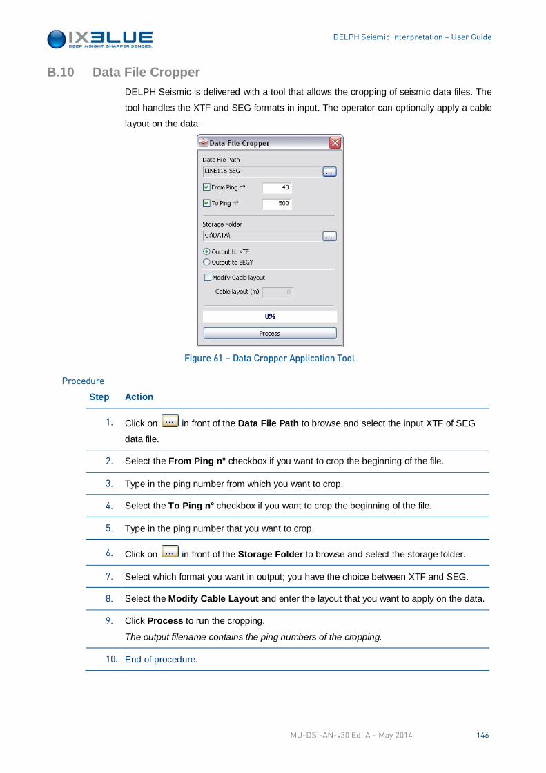
DELPH Seismic Interpretation – User Guide
B.10 Data File Cropper DELPH Seismic is delivered with a tool that allows the cropping of seismic data files. The
tool handles the XTF and SEG formats in input. The operator can optionally apply a cable
layout on the data.
Figure 61 – Data Cropper Application Tool
Step Action
1. Click on in front of the Data File Path to browse and select the input XTF of SEG
data file.
2. Select the From Ping n° checkbox if you want to crop the beginning of the file.
3. Type in the ping number from which you want to crop.
4. Select the To Ping n° checkbox if you want to crop the beginning of the file.
5. Type in the ping number that you want to crop.
6. Click on in front of the Storage Folder to browse and select the storage folder.
7. Select which format you want in output; you have the choice between XTF and SEG.
8. Select the Modify Cable Layout and enter the layout that you want to apply on the data.
9. Click Process to run the cropping.
The output filename contains the ping numbers of the cropping.
10. End of procedure.
Procedure
MU-DSI-AN-v30 Ed. A – May 2014 146
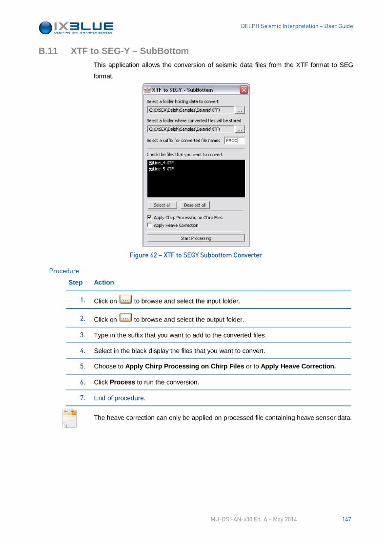
DELPH Seismic Interpretation – User Guide
B.11 XTF to SEG-Y – SubBottom This application allows the conversion of seismic data files from the XTF format to SEG
format.
Figure 62 – XTF to SEGY Subbottom Converter
Step Action
1. Click on to browse and select the input folder.
2. Click on to browse and select the output folder.
3. Type in the suffix that you want to add to the converted files.
4. Select in the black display the files that you want to convert.
5. Choose to Apply Chirp Processing on Chirp Files or to Apply Heave Correction.
6. Click Process to run the conversion.
7. End of procedure.
The heave correction can only be applied on processed file containing heave sensor data.
Procedure
MU-DSI-AN-v30 Ed. A – May 2014 147
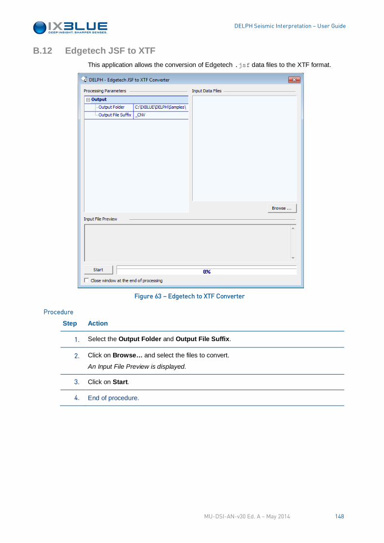
DELPH Seismic Interpretation – User Guide
B.12 Edgetech JSF to XTF This application allows the conversion of Edgetech .jsf data files to the XTF format.
Figure 63 – Edgetech to XTF Converter
Step Action
1. Select the Output Folder and Output File Suffix.
2. Click on Browse… and select the files to convert.
An Input File Preview is displayed.
3. Click on Start.
4. End of procedure.
Procedure
MU-DSI-AN-v30 Ed. A – May 2014 148
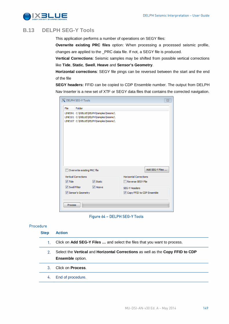
DELPH Seismic Interpretation – User Guide
B.13 DELPH SEG-Y Tools This application performs a number of operations on SEGY files:
Overwrite existing PRC files option: When processing a processed seismic profile,
changes are applied to the _PRC data file. If not, a SEGY file is produced.
Vertical Corrections: Seismic samples may be shifted from possible vertical corrections
like Tide, Static, Swell, Heave and Sensor’s Geometry.
Horizontal corrections: SEGY file pings can be reversed between the start and the end
of the file
SEGY headers: FFID can be copied to CDP Ensemble number. The output from DELPH
Nav Inserter is a new set of XTF or SEGY data files that contains the corrected navigation.
Figure 64 – DELPH SEG-Y Tools
Step Action
1. Click on Add SEG-Y Files … and select the files that you want to process.
2. Select the Vertical and Horizontal Corrections as well as the Copy FFID to CDP Ensemble option.
3. Click on Process.
4. End of procedure.
Procedure
MU-DSI-AN-v30 Ed. A – May 2014 149
DELPH Seismic Interpretation – User Guide
C. UNITS
Distances:
• Inch : 0.0254 meters
• Foot : 0.3048 meters
• Mile : 1609.344 meters
• Fathom : 1.8288 meters
• Yard : 0.9144 meters
• US Survey Inch : 0.02540005080010160342 meters
• US Survey Foot : 0.30480060901219241 meters
• US Survey Mile : 1609.34721869443759248 meters
• US Survey Fathom : 1.828803657607315446 meters
• Nautical Mile : 1852 meters
Speed:
• Knot: 1 Nautical Mile / 3600 second, meter /second with 1 nautical Mile = 1852 meters
Angle:
• Radian: 180 / Pi, with Pi: 3.14159265359
MU-DSI-AN-v30 Ed. A – May 2014 150
Recommended