Download pdf - ECMWF Œ ARM Report Series - ECMWF | Advancing … · ECMWF - ARM Report Series No. 2 ... A recent structural model upgrade has been the introduction of the Eddy ... operational in

ECMWF – ARM Report Series

2. A dual mass flux framework for boundary layerconvection. Part I: Transport

Roel A. J. Neggers, Martin Kohler, Anton C. M. Beljaars

European Centre for Medium-Range Weather ForecastsEuropaisches Zentrum fur mittelfristige WettervorhersageCentre europeen pour les previsions meteorologiques a moyen terme

Series: ECMWF - ARM Report Series

A full list of ECMWF Publications can be found on our web site under:http://www.ecmwf.int/publications/

Contact: [email protected]

c

Copyright 2007

European Centre for Medium Range Weather ForecastsShinfield Park, Reading, RG2 9AX, England

Literary and scientific copyrights belong to ECMWF and are reserved in all countries. This publication is notto be reprinted or translated in whole or in part without the written permission of the Director. Appropriatenon-commercial use will normally be granted under the condition that reference is made to ECMWF.

The information within this publication is given in good faith and considered to be true, but ECMWF acceptsno liability for error, omission and for loss or damage arising from its use.

http://www.ecmwf.int/publications/

ECMWF - ARM Report Series No. 2

A dual mass flux framework for boundary layerconvection. Part I: Transport

Roel A. J. Neggers, Martin Kohler, Anton C. M.Beljaars

March 6, 2007

ARM – Atmospheric Radiation Measurement

A dual mass flux framework for boundary layer convection. Part I: Transport

Abstract

The eddy diffusivity - mass flux (EDMF) approach for turbulent transport in well-mixed layers is extendedinto the modeling of shallow cumulus convection. Model complexity is enhanced to enable representationof conditionally unstable cloud layers that are flexibly coupled to the mixed layer. This significantly expandsthe range of applicability of EDMF, in principle including all major regimes of boundary layer convectionand transitions between those. The treatment of subgrid transport and clouds is integrated by parameterizingboth in terms of the same turbulent joint-distribution. This potentially skewed distribution is reconstructedusing an ensemble of resolved updrafts, rising from the surface layer. Part I of this study concerns theformulation of this multiple updraft framework. A key new ingredient is the application of flexible areapartitioning in the updraft ensemble, which is determined by the coupling between cumulus clouds andthe sub-cloud mixed layer. This is achieved by defining and resolving two specific groups of updrafts;dry mixed-layer updrafts that never reach their lifting condensation level, and moist updrafts that condenseand become positively buoyant cumulus clouds. This technique facilitates the representation of gradualtransitions to and from shallow cumulus convection, and implicitly represents the impact of cloud basetransition layer stability on cumulus transport. Other upgrades include i) flexible updraft entrainment rates,ii) stability feedbacks on the vertical structure of cloudy mass flux, and iii) the introduction of an entrainmentefficiency closure for transport into the cumulus inversion. Impacts of these new components on boundarylayer structure and equilibration are assessed.

1 Introduction

Shallow cumulus convection was first represented in the Integrated Forecasting System (IFS) of the EuropeanCentre for Medium-range Weather Forecasts (ECMWF) by Tiedtke et al. (1988), reporting large but mostlyfavourable impacts on global model climate. Since its introduction, the basic structure of the shallow cumulusscheme has not changed significantly. However, biases in the IFS climate have recently been diagnosed that arerelated to the representation of shallow cumulus convection. A recent intercomparison study of cloud represen-tation in general circulation models (GCM) for the north-east Pacific (Siebesma et al., 2004) illustrates that thecurrent IFS typically predicts too much cloudiness in the subtropical marine Tradewind regions, but too little inthe stratocumulus subsidence areas. Evaluation against observations at the Southern Great Plains (SGP) site ofthe Atmospheric Radiation Measurement (ARM) program (Stokes and Schwartz, 1994; Ackerman and Stokes,2003) has revealed that the occurrence of summertime shallow cumulus is underestimated (Cheinet, 2004), andthat the onset of precipitating convection occurs too early (Mace et al., 1998; Betts and Jakob, 2002). Furtherdetailed evaluation of model physics against large-eddy simulation (LES) has traced some of these shortcom-ings to individual model components. For example, Neggers et al. (2004) illustrated that the moist static energyconvergence closure used in the ECMWF model predicts too vigorous cumulus mass fluxes, directly causingtoo fast deepening cloud and sub-cloud layers and a too fast hydrological cycle.

These issues have motivated a critical reassessment of the representation of the planetary boundary layer (PBL)in IFS. A recent structural model upgrade has been the introduction of the Eddy Diffusivity Mass Flux frame-work (EDMF, Siebesma and Teixeira, 2000; Siebesma et al., 2007) in IFS, as documented by Kohler (2005)and Tompkins et al. (2004). This method combines diffusive and advective models in the parameterization ofturbulent transport, thus making use of the different nature of both techniques. The EDMF scheme as currentlyoperational in IFS is applied to well-mixed layers only, such as the dry convective boundary layer (CBL) andthe stratocumulus topped PBL. This paper presents an extension of EDMF that enables representation of con-ditionally unstable shallow cumulus cloud layers, thus covering all major convective boundary layer regimes.Second target of this project is to improve representation of transitions between such regimes in IFS.

Three important principles define the structure of the shallow cumulus extension. The first is the fact that thetransporting cumulus updrafts are part of a joint-distribution of total specific humidity, potential temperature

ECMWF-ARM Report Series No. 2 1


and vertical velocity that is increasingly skewed with height (e.g. Wyngaard and Moeng, 1992). Any parame-terization of turbulent transport requires reconstruction of this skewed distribution in some way. Theoretically,this requires knowledge of at least three of its lowest statistical moments, which can be explicitly modelled(e.g. Lappen and Randall, 2001; Golaz, 2002). An alternative method resolves skewness by means of multi-ple rising updrafts, each representing a separate segment (or fraction) of the joint PDF (e.g. Kain and Fritsch,1990; Neggers et al., 2002). This technique is also applied here, however additional degrees of freedom areconsciously introduced in various new ways. Key novelty is that each updraft represents an area fraction thatis flexible, as a function of model state. This flexibility subsequently finds its way into updraft initialization atthe surface. As will be shown, this method facilitates representation of transient cloudy boundary layers, andregime transitions in general.

The second defining principle is the explicit representation of the coupling between shallow cumulus cloudsand the sub-cloud mixed layer (e.g. Betts, 1976; Nicholls and LeMone, 1980). Recent studies have revealed theexistence of feedbacks between cumulus mass flux and the stability of the cloud base transition layer (Mapes,2000; Bretherton et al., 2004; Neggers et al., 2004, 2006). We let the nature of this “valve” mechanism de-termine the area partitioning of the updraft ensemble. To this purpose we define and resolve two matchingupdraft groups; one group representing all dry mixed-layer updrafts that stop below cloud base, the other rep-resenting all updrafts that condense and become positively buoyant cumulus clouds. Their area fractions areparameterized, as a function of moist static stability above mixed layer top. These choices have some usefulconsequences. Dry and moist transporting updrafts can now coexist at any time. In combination with flex-ible updraft area partitioning this theoretically enables a gradual onset and decay of cumulus mass flux. Bystopping below cloud base the dry updraft acts to maintain the internal counter-gradient structure of the mixedlayer, as well as the temperature and humidity jumps across the transition layer. Finally, the valve mechanismthus introduced in the mass flux closure always acts to equilibrate the shallow cumulus topped PBL.

The third defining principle of the new extension is an internally consistent treatment of turbulent transportand clouds within the PBL. These are often modeled in separate schemes, which is somewhat at odds withthe fact that clouds and transport in the cumuliform PBL typically refer to the same turbulent eddies, withrelatively short turn-over timescales. This motivates parameterizing both PBL cloudiness and transport interms of the same reconstructed joint-distribution, an approach demonstrated by Lappen and Randall (2001)and Golaz (2002) to enable a unified, integrated representation of subgrid transport and clouds for differentregimes. To this purpose, a bimodal statistical cloud scheme (Lewellen and Yoh, 1993) is attached to theEDMF scheme, in which the total PDF is assumed to consist of two separate, independent Gaussian PDFs;one representing the active (updraft) clouds and one the passive (diffusive) clouds. As this decomposition isequivalent to that defining the EDMF framework, a bimodal PDF scheme thus forms a natural extension ofEDMF into the modelling of clouds.

Part I of this paper is concerned with the formulation of the transport scheme. New model components will beevaluated individually against large eddy simulation (LES) results for prototype shallow cumulus cases, includ-ing steady state and transient scenarios. This supports the parameterizations, and allows realistic calibration ofassociated constants of proportionality. Particular attention will be given to diurnal cycles of shallow cumulusas observed at the ARM SGP site, motivated by the poor represenation of this scenario in IFS. Part II of thispaper presents the extension of the EDMF framework into the statistical representation of sub-grid boundarylayer clouds. Finally, part III presents comprehensive evaluation of the new model. Performance will be evalu-ated against LES and observational datasets, for i) prototype cases, ii) transitional cases, and iii) globally, wheninteractive with the larger scales in the IFS.

The EDMF approach is shortly introduced in sections 2 and 3. The multiple updraft component is formulatedin section 4, and the diffusive component in section 5. The results are further discussed in section 6, and someconcluding remarks are made in 7. Appendix A gives details of the LES code and all cases.

2 ECMWF-ARM Report Series No. 2


2 Conserved state variables

The PBL model is formulated in terms of thermodynamic state variables φ that are conserved for moist adiabaticmotion,

φ qt θl (1)

Here qt is the total specific humidity, defined as

qt qv ql qi (2)

where qv is specific humidity, and ql and qi are specific liquid and ice water content respectively. The otherstate variable θl is the liquid water potential temperature,

θl θ Lvql Lsqi

cpΠ(3)

where θ is potential temperature, cp is the specific heat capacity at constant pressure, Π is the Exner function, Lv

is the specific latent heat of the phase change of evaporation, and Ls that of sublimation. The grid-box averagebudget equation for φ can in short notation be written as

∂φ∂ t ∂ρ w φ

ρ ∂ z

PBL ∂φ

∂ t Ph ∂φ

∂ t LS (4)

where the horizontal overbar indicates a horizontal average over the gridbox, and the prime represents anyperturbation from that average. ρ is air density, subcript Ph indicates the tendency due to all physics not relatedto PBL turbulence, and subscript LS indicates the tendency due to the larger (resolved) scales in the GCM.This paper is only concerned with the parameterization of the PBL turbulent flux w φ and PBL cloud fractionand condensate. For a complete description of all other terms in the budget we refer to the IFS Cycle 31R1documentation (available on the internet at http://www.ecmwf.int/research/ifsdocs/).

3 The eddy diffusivity mass flux (EDMF) framework

The multiple updraft model presented in this study is an extension to the eddy diffusivity mass flux (EDMF)framework, as formulated by Siebesma and Teixeira (2000) and Siebesma et al. (2007). The implementationin the ECMWF model is described by Kohler (2005) and Tompkins et al. (2004). Only a short summary isgiven in this section, for further details we refer to these papers. The remainder of this paper presents the newapproaches and concepts that together form the new extension.

Ertel (1942) was among the first to address the different behaviour of turbulent transport by organized updraftscompared to that by smaller, more random perturbations. While small perturbations tend to do transport in amore diffusive manner (down-gradient), organized updrafts are able to overcome local stability and hence dotransport against local gradients. This has been the motivation for representing counter-gradient transport termsalongside pure diffusive, K-diffusion terms (Holtslag and Moeng, 1991).

Motivated by these arguments a decomposition is made of the total turbulent flux w φ into an advective part byorganized updrafts and a diffusive part by weaker, more random perturbations,

w φ up w φ up K w φ K (5)

where up is the area fraction covered by the organized updrafts, and K 1 up is that covered bythe remaining, “diffusive” air. Based on the typically observed small values of the area fraction covered by



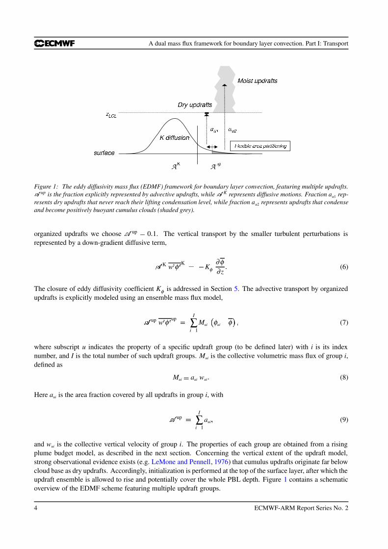
Figure 1: The eddy diffusivity mass flux (EDMF) framework for boundary layer convection, featuring multiple updrafts. up is the fraction explicitly represented by advective updrafts, while K represents diffusive motions. Fraction au1 rep-

resents dry updrafts that never reach their lifting condensation level, while fraction au2 represents updrafts that condenseand become positively buoyant cumulus clouds (shaded grey).

organized updrafts we choose up 0 1. The vertical transport by the smaller turbulent perturbations isrepresented by a down-gradient diffusive term,

K w φ K Kφ∂φ∂ z (6)

The closure of eddy diffusivity coefficient Kφ is addressed in Section 5. The advective transport by organizedupdrafts is explicitly modeled using an ensemble mass flux model,

up w φ up I

∑i 1

Mui φui φ (7)

where subscript u indicates the property of a specific updraft group (to be defined later) with i is its indexnumber, and I is the total number of such updraft groups. Mui is the collective volumetric mass flux of group i,defined as

Mui aui wui (8)

Here aui is the area fraction covered by all updrafts in group i, with

up I

∑i 1

aui (9)

and wui is the collective vertical velocity of group i. The properties of each group are obtained from a risingplume budget model, as described in the next section. Concerning the vertical extent of the updraft model,strong observational evidence exists (e.g. LeMone and Pennell, 1976) that cumulus updrafts originate far belowcloud base as dry updrafts. Accordingly, initialization is performed at the top of the surface layer, after which theupdraft ensemble is allowed to rise and potentially cover the whole PBL depth. Figure 1 contains a schematicoverview of the EDMF scheme featuring multiple updraft groups.



a)

b)

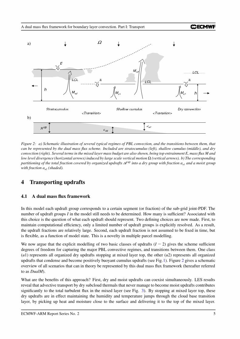
Figure 2: a) Schematic illustration of several typical regimes of PBL convection, and the transitions between them, thatcan be represented by the dual mass flux scheme. Included are stratocumulus (left), shallow cumulus (middle), and dryconvection (right). Several terms in the mixed layer mass budget are also shown, being top entrainment E, mass flux M andlow level divergence (horizontal arrows) induced by large scale vertical motion Ω (vertical arrows). b) The correspondingpartitioning of the total fraction covered by organized updrafts

up into a dry group with fraction au1 and a moist groupwith fraction au2 (shaded).

4 Transporting updrafts

4.1 A dual mass flux framework

In this model each updraft group corresponds to a certain segment (or fraction) of the sub-grid joint-PDF. Thenumber of updraft groups I in the model still needs to be determined. How many is sufficient? Associated withthis choice is the question of what each updraft should represent. Two defining choices are now made. First, tomaintain computational efficiency, only a limited number of updraft groups is explicitly resolved. As a result,the updraft fractions are relatively large. Second, each updraft fraction is not assumed to be fixed in time, butis flexible, as a function of model state. This is a novelty in multiple parcel modelling.

We now argue that the explicit modelling of two basic classes of updrafts (I 2) gives the scheme sufficientdegrees of freedom for capturing the major PBL convective regimes, and transitions between them. One class(u1) represents all organized dry updrafts stopping at mixed layer top, the other (u2) represents all organizedupdrafts that condense and become positively buoyant cumulus updrafts (see Fig.1). Figure 2 gives a schematicoverview of all scenarios that can in theory be represented by this dual mass flux framework (hereafter referredto as DualM).

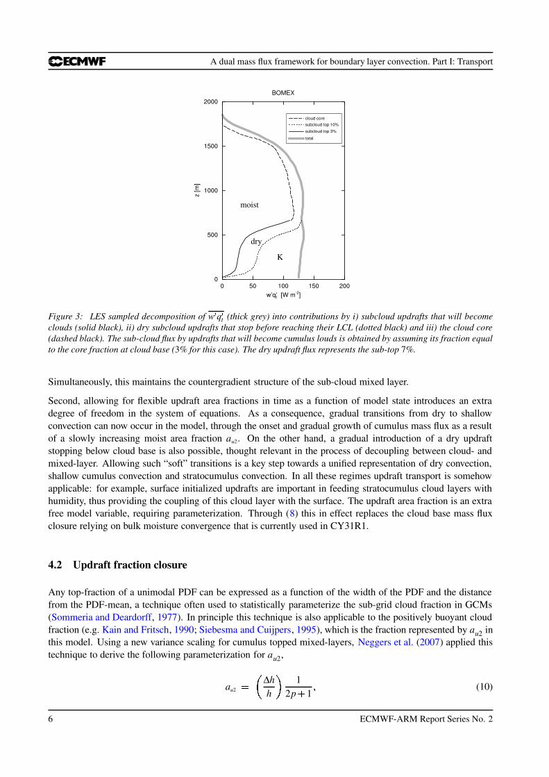
What are the benefits of this approach? First, dry and moist updrafts can coexist simultaneously. LES resultsreveal that advective transport by dry subcloud thermals that never manage to become moist updrafts contributessignificantly to the total turbulent flux in the mixed layer (see Fig. 3). By stopping at mixed layer top, thesedry updrafts are in effect maintaining the humidity and temperature jumps through the cloud base transitionlayer, by picking up heat and moisture close to the surface and delivering it to the top of the mixed layer.



moist

dry

K

Figure 3: LES sampled decomposition of w q t (thick grey) into contributions by i) subcloud updrafts that will becomeclouds (solid black), ii) dry subcloud updrafts that stop before reaching their LCL (dotted black) and iii) the cloud core(dashed black). The sub-cloud flux by updrafts that will become cumulus louds is obtained by assuming its fraction equalto the core fraction at cloud base (3% for this case). The dry updraft flux represents the sub-top 7%.

Simultaneously, this maintains the countergradient structure of the sub-cloud mixed layer.

Second, allowing for flexible updraft area fractions in time as a function of model state introduces an extradegree of freedom in the system of equations. As a consequence, gradual transitions from dry to shallowconvection can now occur in the model, through the onset and gradual growth of cumulus mass flux as a resultof a slowly increasing moist area fraction au2. On the other hand, a gradual introduction of a dry updraftstopping below cloud base is also possible, thought relevant in the process of decoupling between cloud- andmixed-layer. Allowing such “soft” transitions is a key step towards a unified representation of dry convection,shallow cumulus convection and stratocumulus convection. In all these regimes updraft transport is somehowapplicable: for example, surface initialized updrafts are important in feeding stratocumulus cloud layers withhumidity, thus providing the coupling of this cloud layer with the surface. The updraft area fraction is an extrafree model variable, requiring parameterization. Through (8) this in effect replaces the cloud base mass fluxclosure relying on bulk moisture convergence that is currently used in CY31R1.

4.2 Updraft fraction closure

Any top-fraction of a unimodal PDF can be expressed as a function of the width of the PDF and the distancefrom the PDF-mean, a technique often used to statistically parameterize the sub-grid cloud fraction in GCMs(Sommeria and Deardorff, 1977). In principle this technique is also applicable to the positively buoyant cloudfraction (e.g. Kain and Fritsch, 1990; Siebesma and Cuijpers, 1995), which is the fraction represented by au2 inthis model. Using a new variance scaling for cumulus topped mixed-layers, Neggers et al. (2007) applied thistechnique to derive the following parameterization for au2,

au2 ∆hh 1

2p 1 (10)



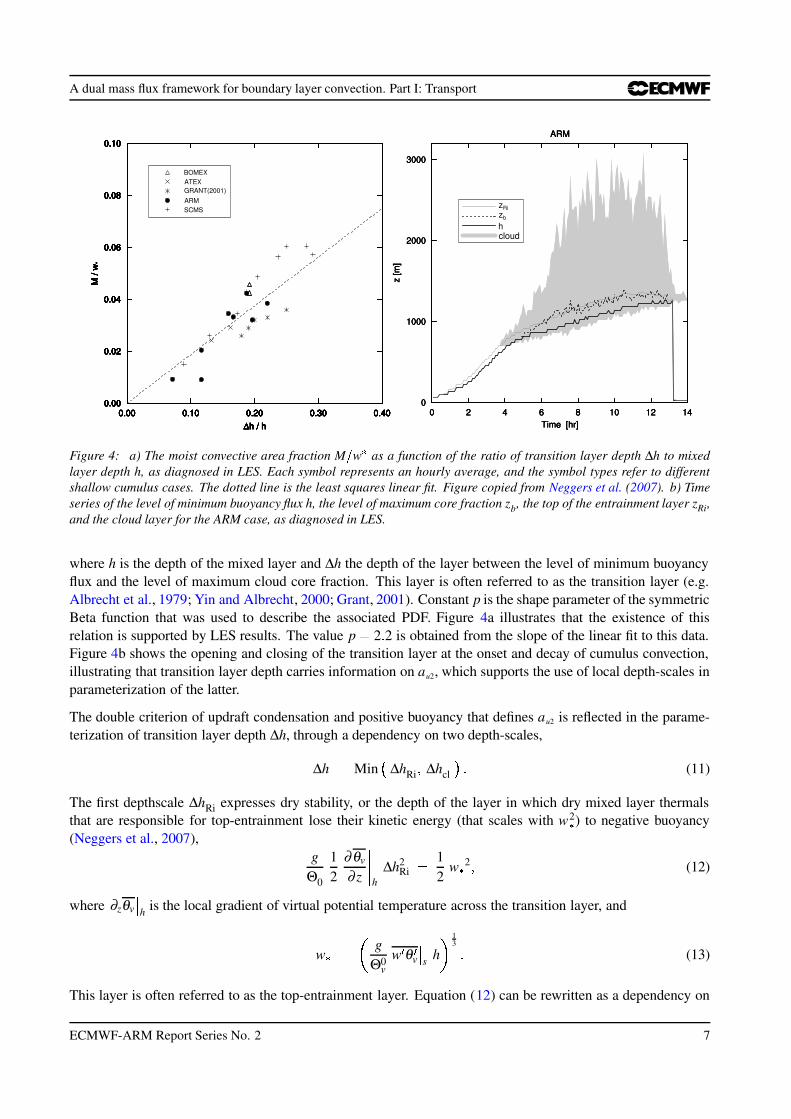
Figure 4: a) The moist convective area fraction M w as a function of the ratio of transition layer depth ∆h to mixedlayer depth h, as diagnosed in LES. Each symbol represents an hourly average, and the symbol types refer to differentshallow cumulus cases. The dotted line is the least squares linear fit. Figure copied from Neggers et al. (2007). b) Timeseries of the level of minimum buoyancy flux h, the level of maximum core fraction zb, the top of the entrainment layer zRi,and the cloud layer for the ARM case, as diagnosed in LES.

where h is the depth of the mixed layer and ∆h the depth of the layer between the level of minimum buoyancyflux and the level of maximum cloud core fraction. This layer is often referred to as the transition layer (e.g.Albrecht et al., 1979; Yin and Albrecht, 2000; Grant, 2001). Constant p is the shape parameter of the symmetricBeta function that was used to describe the associated PDF. Figure 4a illustrates that the existence of thisrelation is supported by LES results. The value p 2 2 is obtained from the slope of the linear fit to this data.Figure 4b shows the opening and closing of the transition layer at the onset and decay of cumulus convection,illustrating that transition layer depth carries information on au2, which supports the use of local depth-scales inparameterization of the latter.

The double criterion of updraft condensation and positive buoyancy that defines au2 is reflected in the parame-terization of transition layer depth ∆h, through a dependency on two depth-scales,

∆h Min ∆hRi ∆hcl (11)

The first depthscale ∆hRi expresses dry stability, or the depth of the layer in which dry mixed layer thermalsthat are responsible for top-entrainment lose their kinetic energy (that scales with w2 ) to negative buoyancy(Neggers et al., 2007),

gΘ0

12

∂θv

∂ z

h

∆h2Ri 1

2w 2 (12)

where ∂zθvh is the local gradient of virtual potential temperature across the transition layer, and

w g

Θ0v

w θ v s h 13 (13)

This layer is often referred to as the top-entrainment layer. Equation (12) can be rewritten as a dependency on



the interfacial Richardson number Rih,

∆hRih 1

Rih Rih g

Θv∆θ h

v h

w 2 (14)

This makes parameterization (10) commensurate with the equilibrium scaling of Stevens (2006) and the LESresults of Grant (2006), both suggesting a mass flux dependence on the inverse Richardson number. The seconddepthscale ∆hcl introduces dependency on the occurrence of condensation in rising thermals at mixed layer top(Neggers et al., 2004, 2006). This cumulus instability depthscale is parameterized proportional to the cloudydepth of a strong, non-transporting test updraft (i 0 au0 0 02),

∆hcl γ ztopu0 zlcl

u0 (15)

Figure 4b illustrates that ∆h correlates well with convective cloud depth, suggesting γ 0 15. This correlationexpresses the impact of transition layer stability on the vertical velocity budget of a rising cloudy updraft,affecting the eventual height it reaches. Parameterization (15) is therefore most applicable to forced convection,in which the impact of transition layer stability on convective cloud depth is not yet obscured by latent heatrelease.

Stability and condensation above mixed layer top thus together determine the moist area fraction in the model.Taking the minimum of both depth-scales ensures that both criteria can constrain au2. This is illustrated in Fig.4b, showing the time-development of both depth-scales during an LES simulation of a diurnal cycle of shallowcumulus at ARM SGP. The top of the entrainment layer zRi is obtained by vertically integrating moist staticstability (∆θv) above h until equation (12) is met. The depth of the entrainment layer ∆hRi matches transitionlayer depth ∆h reasonably well in the period of significant convective cloud depth. However, as ∆hRi reflects theovershooting depth of dry thermals, it is always non-zero, also in the dry CBL. This motivates the superpositionof an additional criterion reflecting updraft condensation. The main role of this depth-scale ∆hcl is to ensurethat the moist updraft area fraction goes to zero for the dry convective limit

limztop

u0 zlclu0 0

au2 0 (16)

The definition of mass flux (8) means that the same limit applies to Mu2. Depth scale ∆hcl therefore reproducespotentially gradual transitions between the dry CBL and the shallow cumulus topped PBL. Numerical benefitof (15) over (12) in this respect is that cumulus depth is typically better resolved than jump ∆θ h

v .

As w is typically about 1 m/s, Mu2 will be sensitive to au2. Area fractions of only a few percent already createsufficiently large cumulus (mass)fluxes to balance the large scale forcings in the cloud layer. The dependenceof au2 on stability and updraft condensation thus introduces new feedbacks in the transport scheme betweencumulus transport and the subcloud mixed layer. This mechanism acts to equilibrate the boundary layer, as willbe illustrated in section 6.

4.3 Flexible updraft initialization

The next step is to apply the flexible area fractions of the updrafts, as parameterized in the previous section, intheir surface initialization. To this purpose these fractions are assumed constant with height throughout the sub-cloud mixed layer. As a consequence, at the surface the moist fraction au2 represents the fraction of the updraftsthat will make it through the mixed layer and manage to condense and become buoyant cumulus clouds. Afirst-guess of the area fraction of buoyant cumulus updrafts at cloud base thus determines the partitioning of theupdraft ensemble and its surface initialization.



a) b)

c) d)

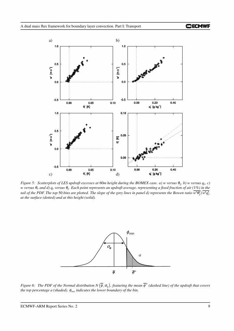
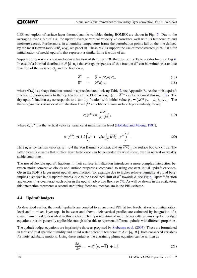
Figure 5: Scatterplots of LES updraft excesses at 60m height during the BOMEX case. a) w versus θl , b) w versus qt , c)w versus θv and d) qt versus θl . Each point represents an updraft average, representing a fixed fraction of air (1%) in thetail of the PDF. The top 50 bins are plotted. The slope of the grey lines in panel d) represents the Bowen ratio w θ l w q t ,at the surface (dotted) and at this height (solid).

a

a

σ!"

min

Figure 6: The PDF of the Normal distribution N # φ $ σφ % , featuring the mean φ a (dashed line) of the updraft that coversthe top percentage a (shaded). φmin indicates the lower boundary of the bin.



LES scatterplots of surface layer thermodynamic variables during BOMEX are shown in Fig. 5. Due to theaveraging over a bin of 1%, the updraft average vertical velocity wi correlates well with its temperature andmoisture excess. Furthermore, in a humidity-temperature frame the perturbation points fall on the line definedby the local Bowen ratio w θ l & w q t , see panel d). These results support the use of reconstructed joint-PDFs forinitialization of model updrafts that represent a similar finite fraction of air.

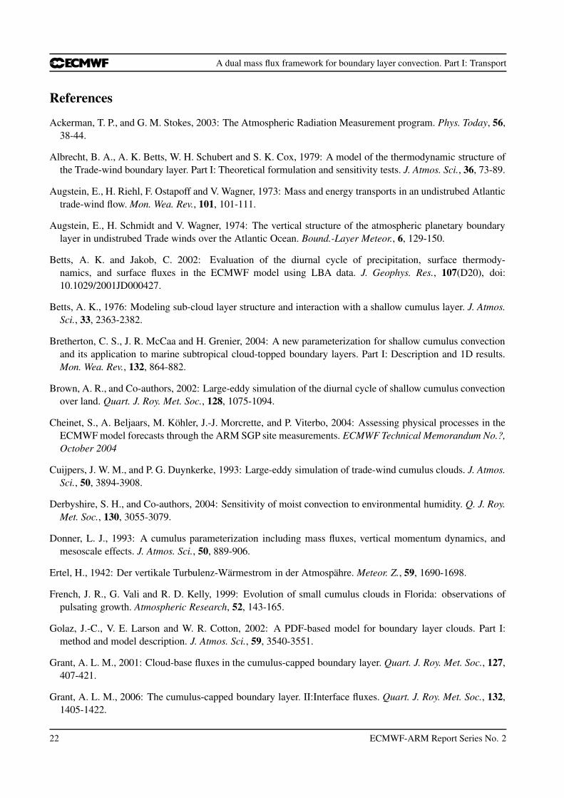
Suppose a represents a certain top area fraction of the joint PDF that lies on the Bowen ratio line, see Fig.6.In case of a Normal distribution N φ σφ the average properties of this fraction φ a can be written as a uniquefunction of the variance σφ and the fraction a,

φ a φ ('*) a + σφ (17)

wa '*) a + σw (18)

where ',) a + is a shape function stored in a precalculated look-up Table 2, see Appendix B. As the moist updraftfraction au2 corresponds to the top fraction of the PDF, average φu2 φ au2 can be obtained through (17). Thedry updraft fraction au1 corresponds to a sub-top fraction with initial value φu1 ) upφup au2φu2 + & au1. Thethermodynamic variances at initialization level zini are obtained from surface layer similarity theory,

σφ ) zini + w φ sσw ) zini + (19)

where σw ) zini + is the vertical velocity variance at initialization level (Holtslag and Moeng, 1991),

σw ) zini + 1 2 u3 1 5κg

Θ0v

w θ v s zini 13 (20)

Here u is the friction velocity, κ 0 4 the Von Karman constant, and gΘ0

vw θ v s the surface buoyancy flux. The

latter formula ensures that surface layer turbulence can be generated by wind shear, even in neutral or weaklystable conditions.

The use of flexible updraft fractions in their surface initialization introduces a more complex interaction be-tween moist convective clouds and surface properties, compared to using constant initial updraft excesses.Given the PDF, a larger moist updraft area fraction (for example due to higher relative humidity at cloud base)implies a smaller initial updraft excess, due to the associated shift of φ a towards φ , see Fig.6. Updraft fractionand excess thus counteract each other in the updraft advective flux, see (7). As will be shown in the evaluation,this interaction represents a second stabilizing feedback mechanism in the PBL scheme.

4.4 Updraft budgets

As described earlier, the model updrafts are coupled to an assumed PDF at two levels, at surface initializationlevel and at mixed layer top. In between and above, their vertical profiles are estimated by integration of arising plume model, described in this section. The representation of multiple updrafts requires updraft budgetequations that are generally applicable enough to be able to represent different updrafts with different properties.

The updraft budget equations are in principle those as proposed by Siebesma et al. (2007). These are formulatedin terms of total specific humidity and liquid water potential temperature φ - qt θl , both conserved variablesfor moist adiabatic motions. Using these variables the entraining plume equation can be written as

∂φui

∂ z εφui φui φ µφ

ui (21)



a)

b)

c)

d)

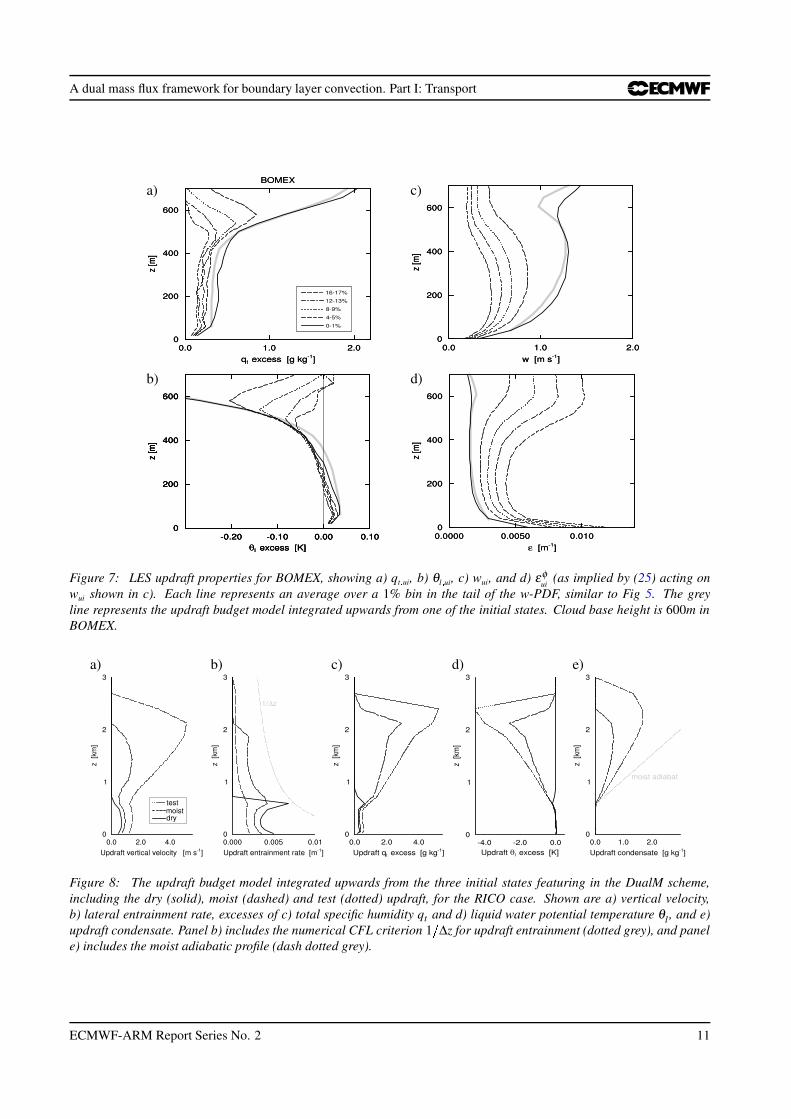
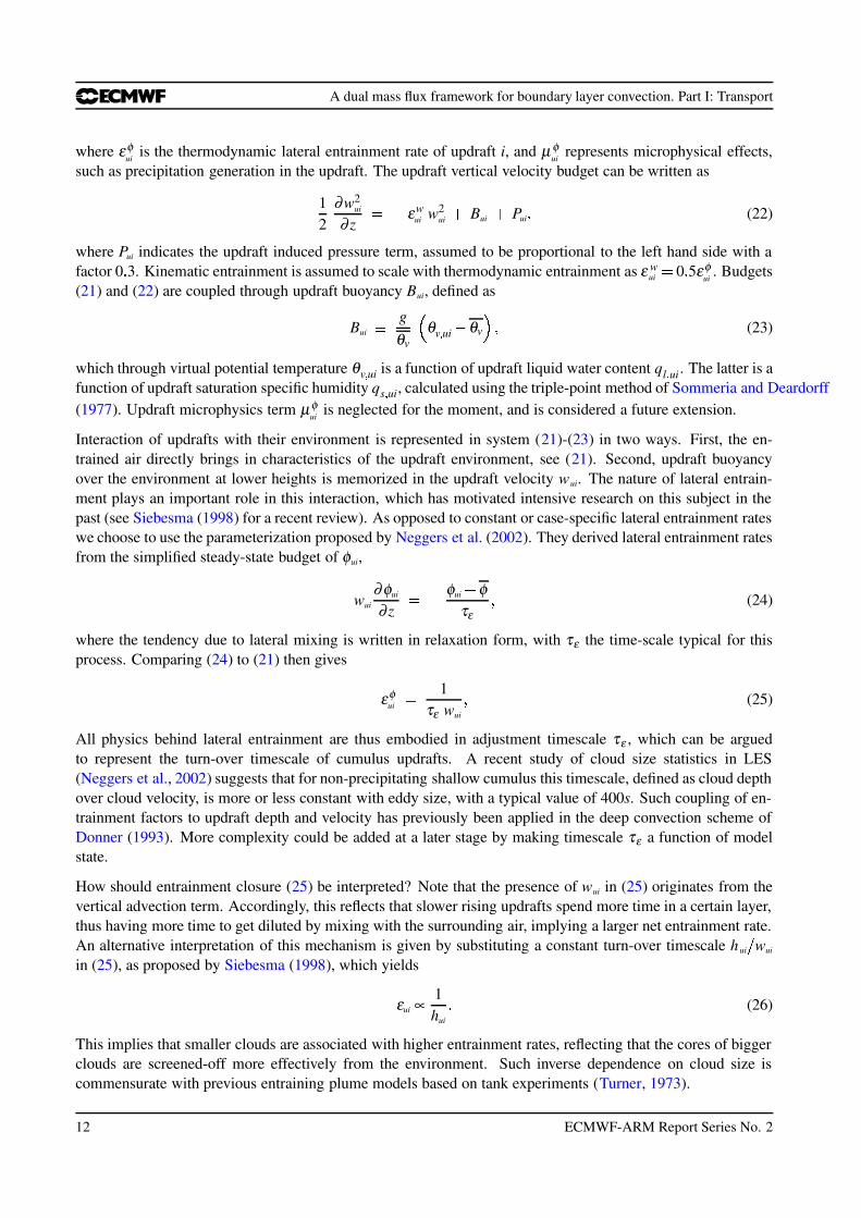
Figure 7: LES updraft properties for BOMEX, showing a) qt . ui, b) θl . ui, c) wui, and d) εφui

(as implied by (25) acting onwui shown in c). Each line represents an average over a 1% bin in the tail of the w-PDF, similar to Fig 5. The greyline represents the updraft budget model integrated upwards from one of the initial states. Cloud base height is 600m inBOMEX.

a) b) c) d) e)

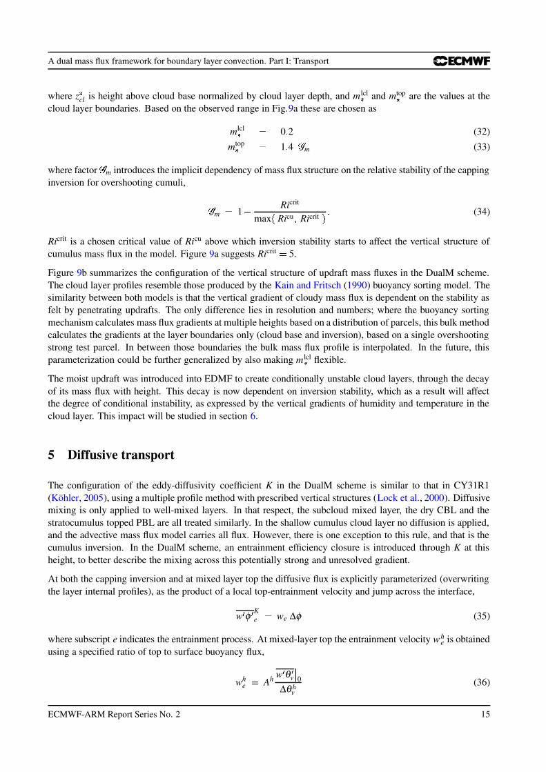
Figure 8: The updraft budget model integrated upwards from the three initial states featuring in the DualM scheme,including the dry (solid), moist (dashed) and test (dotted) updraft, for the RICO case. Shown are a) vertical velocity,b) lateral entrainment rate, excesses of c) total specific humidity qt and d) liquid water potential temperature θl , and e)updraft condensate. Panel b) includes the numerical CFL criterion 1 ∆z for updraft entrainment (dotted grey), and panele) includes the moist adiabatic profile (dash dotted grey).



where εφui is the thermodynamic lateral entrainment rate of updraft i, and µ φ

ui represents microphysical effects,such as precipitation generation in the updraft. The updraft vertical velocity budget can be written as

12

∂w2ui

∂ z εwui w2

ui Bui Pui (22)

where Pui indicates the updraft induced pressure term, assumed to be proportional to the left hand side with afactor 0 3. Kinematic entrainment is assumed to scale with thermodynamic entrainment as ε w

ui 0 5εφui . Budgets

(21) and (22) are coupled through updraft buoyancy Bui, defined as

Bui gθv / θv0 ui θv 1 (23)

which through virtual potential temperature θv0 ui is a function of updraft liquid water content ql 0 ui . The latter is afunction of updraft saturation specific humidity qs 0 ui, calculated using the triple-point method of Sommeria and Deardorff(1977). Updraft microphysics term µ φ

ui is neglected for the moment, and is considered a future extension.

Interaction of updrafts with their environment is represented in system (21)-(23) in two ways. First, the en-trained air directly brings in characteristics of the updraft environment, see (21). Second, updraft buoyancyover the environment at lower heights is memorized in the updraft velocity wui. The nature of lateral entrain-ment plays an important role in this interaction, which has motivated intensive research on this subject in thepast (see Siebesma (1998) for a recent review). As opposed to constant or case-specific lateral entrainment rateswe choose to use the parameterization proposed by Neggers et al. (2002). They derived lateral entrainment ratesfrom the simplified steady-state budget of φui,

wui

∂φui

∂ z φui φτε

(24)

where the tendency due to lateral mixing is written in relaxation form, with τε the time-scale typical for thisprocess. Comparing (24) to (21) then gives

εφui 1

τε wui (25)

All physics behind lateral entrainment are thus embodied in adjustment timescale τε , which can be arguedto represent the turn-over timescale of cumulus updrafts. A recent study of cloud size statistics in LES(Neggers et al., 2002) suggests that for non-precipitating shallow cumulus this timescale, defined as cloud depthover cloud velocity, is more or less constant with eddy size, with a typical value of 400s. Such coupling of en-trainment factors to updraft depth and velocity has previously been applied in the deep convection scheme ofDonner (1993). More complexity could be added at a later stage by making timescale τε a function of modelstate.

How should entrainment closure (25) be interpreted? Note that the presence of wui in (25) originates from thevertical advection term. Accordingly, this reflects that slower rising updrafts spend more time in a certain layer,thus having more time to get diluted by mixing with the surrounding air, implying a larger net entrainment rate.An alternative interpretation of this mechanism is given by substituting a constant turn-over timescale h ui & wui

in (25), as proposed by Siebesma (1998), which yields

εui ∝1hui (26)

This implies that smaller clouds are associated with higher entrainment rates, reflecting that the cores of biggerclouds are screened-off more effectively from the environment. Such inverse dependence on cloud size iscommensurate with previous entraining plume models based on tank experiments (Turner, 1973).



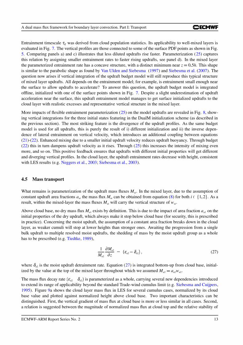
Entrainment timescale τε was derived from cloud population statistics. Its applicability to well-mixed layers isevaluated in Fig. 7. The vertical profiles are those connected to some of the surface PDF points as shown in Fig.5. Comparing panels a) and c) illustrates that less diluted updrafts rise faster. Parameterization (25) capturesthis relation by assigning smaller entrainment rates to faster rising updrafts, see panel d). In the mixed layerthe parameterized entrainment rate has a concave structure, with a distinct minimum near z 0 5h. This shapeis similar to the parabolic shape as found by Van Ulden and Siebesma (1997) and Siebesma et al. (2007). Thequestion now arises if vertical integration of the updraft budget model will still reproduce this typical structureof mixed layer updrafts. All depends on the entrainment model; for example, is entrainment small enough nearthe surface to allow updrafts to accelerate? To answer this question, the updraft budget model is integratedoffline, initialized with one of the surface points shown in Fig. 7. Despite a slight underestimation of updraftacceleration near the surface, this updraft entrainment model manages to get surface initialized updrafts to thecloud layer with realistic excesses and representative vertical structure in the mixed layer.

More impacts of flexible entrainment parameterization (25) on the model updrafts are revealed in Fig. 8, show-ing vertical integrations for the three initial states featuring in the DualM initialization scheme (as described inthe previous section). The most striking feature is the divergence of the updraft profiles. As the same budgetmodel is used for all updrafts, this is purely the result of i) different initialization and ii) the inverse depen-dence of lateral entrainment on vertical velocity, which introduces an additional coupling between equations(21)-(22). Enhanced mixing due to a smaller initial updraft velocity reduces updraft buoyancy. Through budget(22) this in turn dampens updraft velocity as it rises. Through (25) this increases the intensity of mixing evenmore, and so on. This positive feedback ensures that updrafts with different initial properties will get differentand diverging vertical profiles. In the cloud layer, the updraft entrainment rates decrease with height, consistentwith LES results (e.g. Neggers et al., 2003; Siebesma et al., 2003).

4.5 Mass transport

What remains is parameterization of the updraft mass fluxes Mui. In the mixed layer, due to the assumption ofconstant updraft area fractions aui the mass flux Mui can be obtained from equation (8) for both i 2 1 2 . As aresult, within the mixed-layer the mass fluxes Mui will carry the vertical structure of wui.

Above cloud base, no dry mass flux Mu1 exists by definition. This is due to the impact of area fraction au1 on theinitial properties of the dry updraft, which always make it stop below cloud base (for security, this is prescribedin practice). Concerning the moist updraft, the assumption of a constant area fraction breaks down in the cloudlayer, as weaker cumuli will stop at lower heights than stronger ones. Awaiting the progression from a singlebulk updraft to multiple resolved moist updrafts, the shedding of mass by the moist updraft group as a wholehas to be prescribed (e.g. Tiedtke, 1989),

1Mu2

∂Mu2

∂ z ) εu2 δu2 + (27)

where δu2 is the moist updraft detrainment rate. Equation (27) is integrated bottom-up from cloud base, initial-ized by the value at the top of the mixed layer throughout which we assumed Mu2 au2wu2.

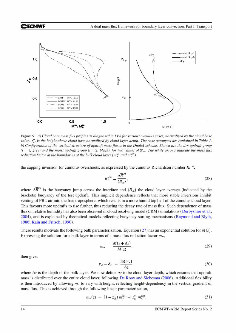
The mass flux decay rate ) εu2 δu2 + is parameterized as a whole, carrying several new dependencies introducedto extend its range of applicability beyond the standard Trade-wind cumulus limit (e.g. Siebesma and Cuijpers,1995). Figure 9a shows the cloud layer mass flux in LES for several cumulus cases, normalized by its cloudbase value and plotted against normalized height above cloud base. Two important characteristics can bedistinguished. First, the vertical gradient of mass flux at cloud base is more or less similar in all cases. Second,a relation is suggested between the magnitude of normalized mass flux at cloud top and the relative stability of



Figure 9: a) Cloud core mass flux profiles as diagnosed in LES for various cumulus cases, normalized by the cloud basevalue. z cl is the height above cloud base normalized by cloud layer depth. The case acronyms are explained in Table 1.b) Configuration of the vertical structure of updraft mass fluxes in the DualM scheme. Shown are the dry updraft group(i 3 1, grey) and the moist updraft group (i 3 2, black), for two values of 4 m. The white arrows indicate the mass fluxreduction factor at the boundaries of the bulk cloud layer (mlcl and mtop ).

the capping inversion for cumulus overshoots, as expressed by the cumulus Richardson number Ricu,

Ricu ∆Bcu5Bu0 6 (28)

where ∆Bcu is the buoyancy jump across the interface and5Bu0 6 the cloud layer average (indicated by the

brackets) buoyancy of the test updraft. This implicit dependence reflects that more stable inversions inhibitventing of PBL air into the free troposphere, which results in a more humid top half of the cumulus cloud layer.This favours more updrafts to rise further, thus reducing the decay rate of mass flux. Such dependence of massflux on relative humidity has also been observed in cloud resolving model (CRM) simulations (Derbyshire et al.,2004), and is explained by theoretical models reflecting buoyancy sorting mechanisms (Raymond and Blyth,1986; Kain and Fritsch, 1990).

These results motivate the following bulk parameterization. Equation (27) has an exponential solution for M ) z + .Expressing the solution for a bulk layer in terms of a mass flux reduction factor m ,

m M ) z ∆z +M ) z + (29)

then gives

εu2 δu2 ln ) m +∆z (30)

where ∆z is the depth of the bulk layer. We now define ∆z to be cloud layer depth, which ensures that updraftmass is distributed over the entire cloud layer, following De Rooy and Siebesma (2006). Additional flexibilityis then introduced by allowing m to vary with height, reflecting height-dependency in the vertical gradient ofmass flux. This is achieved through the following linear parameterization,

m ) z + ) 1 zcl + mlcl z

cl mtop (31)



where zcl is height above cloud base normalized by cloud layer depth, and mlcl and mtop are the values at the

cloud layer boundaries. Based on the observed range in Fig.9a these are chosen as

mlcl 0 2 (32)

mtop 1 4 7 m (33)

where factor 7 m introduces the implicit dependency of mass flux structure on the relative stability of the cappinginversion for overshooting cumuli,

7 m 1 Ricrit

max ) Ricu Ricrit + (34)

Ricrit is a chosen critical value of Ricu above which inversion stability starts to affect the vertical structure ofcumulus mass flux in the model. Figure 9a suggests Ricrit 5.

Figure 9b summarizes the configuration of the vertical structure of updraft mass fluxes in the DualM scheme.The cloud layer profiles resemble those produced by the Kain and Fritsch (1990) buoyancy sorting model. Thesimilarity between both models is that the vertical gradient of cloudy mass flux is dependent on the stability asfelt by penetrating updrafts. The only difference lies in resolution and numbers; where the buoyancy sortingmechanism calculates mass flux gradients at multiple heights based on a distribution of parcels, this bulk methodcalculates the gradients at the layer boundaries only (cloud base and inversion), based on a single overshootingstrong test parcel. In between those boundaries the bulk mass flux profile is interpolated. In the future, thisparameterization could be further generalized by also making mlcl flexible.

The moist updraft was introduced into EDMF to create conditionally unstable cloud layers, through the decayof its mass flux with height. This decay is now dependent on inversion stability, which as a result will affectthe degree of conditional instability, as expressed by the vertical gradients of humidity and temperature in thecloud layer. This impact will be studied in section 6.

5 Diffusive transport

The configuration of the eddy-diffusivity coefficient K in the DualM scheme is similar to that in CY31R1(Kohler, 2005), using a multiple profile method with prescribed vertical structures (Lock et al., 2000). Diffusivemixing is only applied to well-mixed layers. In that respect, the subcloud mixed layer, the dry CBL and thestratocumulus topped PBL are all treated similarly. In the shallow cumulus cloud layer no diffusion is applied,and the advective mass flux model carries all flux. However, there is one exception to this rule, and that is thecumulus inversion. In the DualM scheme, an entrainment efficiency closure is introduced through K at thisheight, to better describe the mixing across this potentially strong and unresolved gradient.

At both the capping inversion and at mixed layer top the diffusive flux is explicitly parameterized (overwritingthe layer internal profiles), as the product of a local top-entrainment velocity and jump across the interface,

w φ Ke we ∆φ (35)

where subscript e indicates the entrainment process. At mixed-layer top the entrainment velocity whe is obtained

using a specified ratio of top to surface buoyancy flux,

whe Ah w θ v 0

∆θ hv

(36)



where Ah is a constant of proportionality, usually assumed 0 2 based on LES simulations (e.g. Stevens, 2006).At mixed layer top, an internal boundary within the cumulus PBL, mass flux exists alongside diffusion. Incontrast, at the cumulus inversion only diffusive transport is allowed; the mass flux in that model-layer isreplaced by a diffusive flux following (35), with the associated cumulus top-entrainment rate wcu

e parameterizedin a similar format as (36),

wcue Acu 8 w θ v 9

∆θ cuv (37)

Here 8 w θ v 9 is the cloud layer average buoyancy flux and Acu is a constant of proportionality, shown byWyant et al. (1997) to be 0 4 using CRM simulations of a stratocumulus to shallow cumulus transition. Trans-port by overshooting cumuli into the capping inversion layer is thus completely represented by the diffusivecomponent of EDMF.

The similarity between (36) and (37) is that both top-entrainment rates are a function of a bulk layer averagebuoyancy flux and an interface buoyancy jump. Rewriting in terms of bulk Richardson numbers (14) and (28)gives

whe Ah

Rihw and wcu

e Acu

Ricu 8 Mu2 9 (38)

respectively, where 8 Mu2 9 is the cloud layer average mass flux. These inverse Richardson numbers act as en-trainment efficiencies, limiting the entrainment rate when local inversion stability ∆θv gets effective in reducingthe kinetic energy of overshooting updrafts. Such techniques show better skill than advective-type models in re-producing transport in strong, unresolved inversions. We thus make full use of the possibility offered by EDMFto combine diffusive and advective transport, emphasizing the representation of one of the two whenever thisis numerically or conceptionally desirable.

6 Discussion

For a comprehensive evaluation of the DualM scheme we refer to Part III of this study. However, some keyimpacts of new model components will now briefly be assessed using the single column model (SCM) setup.Simulations of some prototype shallow cumulus cases are performed during which the cloud scheme is switchedoff, giving insight into the behaviour of the transport model alone. The small cloud fraction and condensatevalues typical of shallow cumulus convection have relatively little impact on the radiative budget, which justifiesthis method. In these simulations the updraft buoyancy term is the only place where condensation has an impact.

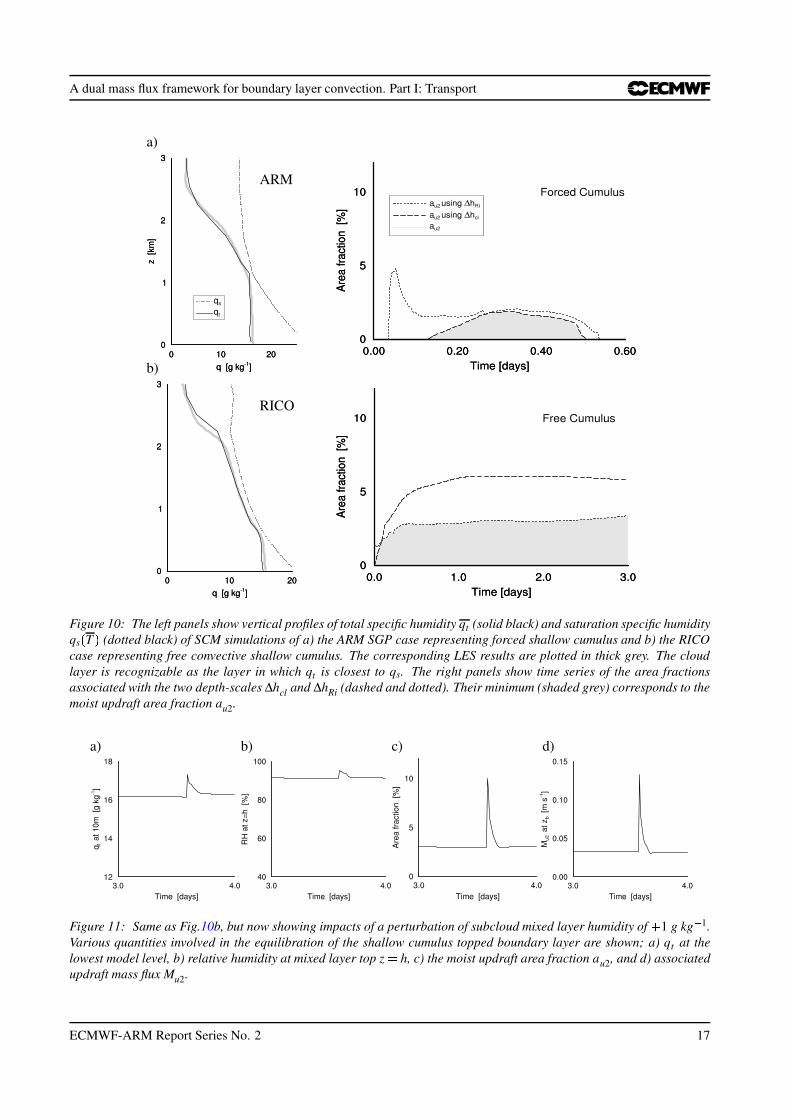
First the parameterization of the moist updraft area fraction au2 is evaluated for two very different shallowcumulus scenarios; a forced shallow cumulus case (ARM SGP) and a free convective shallow cumulus case(RICO). The vertical structure of both cases is reproduced satisfactorily by the transport scheme, see Fig. 10.The degree of convective freedom is reflected in cloud layer depth, which in the RICO case is much deeperas in the ARM case. Figure 10 shows timeseries of depth-scales ∆hcl and ∆hRi for both scenarios. One coulduse the criterion ∆hRi : ∆hcl as the definition of free cumulus convection. In the forced case, ∆hcl nevermanages to become larger than ∆hRi, and thus limits au2. This shows that the system always remains close tothe dry convective limit (16). The benefit of ∆hcl is that moist updraft depth is well resolved, ensuring gradualtransitions from dry to moist convection, as illustrated by the slow increase and decrease of au2 at cloud layeronset and decay in Fig. 10a. In the free convective case, ∆hRi limits au2. In this scenario the cloudy depth of theupdraft no longer uniquely reflects transition layer impacts on updraft buoyancy, as these get overshadowed bythe impact of latent heat release in deeper cloud layers. Taking the minimum of both depth-scales thus ensuresthat the most appropriate scale is automatically chosen.



a)

b)

ARM

RICO

Figure 10: The left panels show vertical profiles of total specific humidity qt (solid black) and saturation specific humidityqs ; T < (dotted black) of SCM simulations of a) the ARM SGP case representing forced shallow cumulus and b) the RICOcase representing free convective shallow cumulus. The corresponding LES results are plotted in thick grey. The cloudlayer is recognizable as the layer in which qt is closest to qs. The right panels show time series of the area fractionsassociated with the two depth-scales ∆hcl and ∆hRi (dashed and dotted). Their minimum (shaded grey) corresponds to themoist updraft area fraction au2.

a) b) c) d)

Figure 11: Same as Fig.10b, but now showing impacts of a perturbation of subcloud mixed layer humidity of = 1 g kg > 1.Various quantities involved in the equilibration of the shallow cumulus topped boundary layer are shown; a) qt at thelowest model level, b) relative humidity at mixed layer top z 3 h, c) the moist updraft area fraction au2, and d) associatedupdraft mass flux Mu2.



a) b)

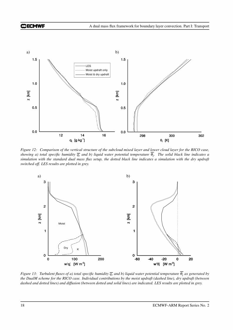
Figure 12: Comparison of the vertical structure of the subcloud mixed layer and lower cloud layer for the RICO case,showing a) total specific humidity qt and b) liquid water potential temperature θl . The solid black line indicates asimulation with the standard dual mass flux setup, the dotted black line indicates a simulation with the dry updraftswitched off. LES results are plotted in grey.

a) b)

Figure 13: Turbulent fluxes of a) total specific humidity qt and b) liquid water potential temperature θl as generated bythe DualM scheme for the RICO case. Individual contributions by the moist updraft (dashed line), dry updraft (betweendashed and dotted lines) and diffusion (between dotted and solid lines) are indicated. LES results are plotted in grey.



a) b)

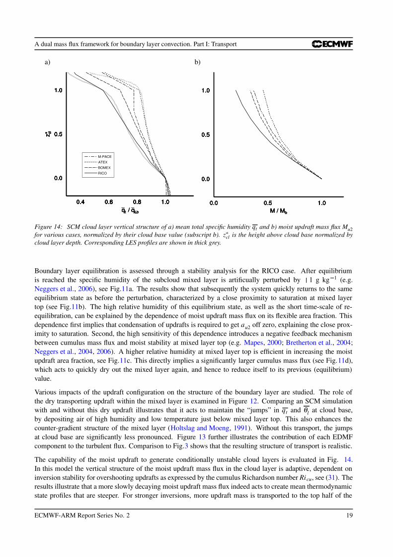
Figure 14: SCM cloud layer vertical structure of a) mean total specific humidity qt and b) moist updraft mass flux Mu2for various cases, normalized by their cloud base value (subscript b). z cl is the height above cloud base normalized bycloud layer depth. Corresponding LES profiles are shown in thick grey.

Boundary layer equilibration is assessed through a stability analysis for the RICO case. After equilibriumis reached the specific humidity of the subcloud mixed layer is artificually perturbed by 1 g kg 1 (e.g.Neggers et al., 2006), see Fig.11a. The results show that subsequently the system quickly returns to the sameequilibrium state as before the perturbation, characterized by a close proximity to saturation at mixed layertop (see Fig.11b). The high relative humidity of this equilibrium state, as well as the short time-scale of re-equilibration, can be explained by the dependence of moist updraft mass flux on its flexible area fraction. Thisdependence first implies that condensation of updrafts is required to get au2 off zero, explaining the close prox-imity to saturation. Second, the high sensitivity of this dependence introduces a negative feedback mechanismbetween cumulus mass flux and moist stability at mixed layer top (e.g. Mapes, 2000; Bretherton et al., 2004;Neggers et al., 2004, 2006). A higher relative humidity at mixed layer top is efficient in increasing the moistupdraft area fraction, see Fig.11c. This directly implies a significantly larger cumulus mass flux (see Fig.11d),which acts to quickly dry out the mixed layer again, and hence to reduce itself to its previous (equilibrium)value.

Various impacts of the updraft configuration on the structure of the boundary layer are studied. The role ofthe dry transporting updraft within the mixed layer is examined in Figure 12. Comparing an SCM simulationwith and without this dry updraft illustrates that it acts to maintain the “jumps” in qt and θl at cloud base,by depositing air of high humidity and low temperature just below mixed layer top. This also enhances thecounter-gradient structure of the mixed layer (Holtslag and Moeng, 1991). Without this transport, the jumpsat cloud base are significantly less pronounced. Figure 13 further illustrates the contribution of each EDMFcomponent to the turbulent flux. Comparison to Fig.3 shows that the resulting structure of transport is realistic.

The capability of the moist updraft to generate conditionally unstable cloud layers is evaluated in Fig. 14.In this model the vertical structure of the moist updraft mass flux in the cloud layer is adaptive, dependent oninversion stability for overshooting updrafts as expressed by the cumulus Richardson number Ricu, see (31). Theresults illustrate that a more slowly decaying moist updraft mass flux indeed acts to create mean thermodynamicstate profiles that are steeper. For stronger inversions, more updraft mass is transported to the top half of the



cloud layer, resulting in a smaller qt gradient. This feature is in accordance with LES results. Such strongerconvergence of specific humidity flux below the inversion favours formation of capping stratus layers, enablingrepresentation of scenarios featuring cumuli rising into stratocumulus. This will be further explored in Part IIof this paper.

7 Concluding remarks

In this study the complexity of the EDMF framework is enhanced to allow representation of more complexPBL scenario’s. A set of modifications is proposed, argued to introduce sufficient extra degrees of freedomto represent shallow cumulus convection, and transitions to and from this PBL regime. The most importantmodification is the introduction of multiple updrafts. The moist updraft is configured to enable representation ofconditionally unstable cloud layers that are flexibly rooted in the subcloud mixed layer. Rooting is representedthrough flexible updraft i) area fraction and ii) surface initialization, both a function of model state. Theproperties of the air transported out of the mixed layer by the cumulus updraft are affected by the mixedlayer through lateral entrainment, which through an inverse dependence on vertical velocity introduces strongsensitivity to the updraft environment. The degree of conditional instability of the cloud layer is controlled bythe stability of the capping inversion for overshooting updrafts, through an adaptive vertical structure of moistupdraft mass flux. Finally, it is demonstrated that the multiple updraft framework facilitates representation ofmoist convective inhibition mechanisms.

The diurnal cycle of shallow cumulus over land has played a key role in the formulation of this model. Within24 hours the boundary layer goes through various very different phases; first a stable situation at dawn, fol-lowed by a dry convective period, followed by forced shallow cumulus developing into free convective shallowcumulus, and finally back to a slowly re-stabilizing residual PBL after dusk. The transience of such complexscenarios requires sufficient model complexity to allow its representation. This illustrates the important rolethat observational data such as provided by the ARM program can play in model development, from supportingLES/CRM simulations, via evaluation of parameterizations at physics level and their subsequent improvement,to evaluation of model climate of GCMs.

The extension of the EDMF framework into the statistical modelling of boundary layer clouds and condensateis presented in Part II of this paper. Among others, the benefits of an internally consistent, bimodal treatment oftransport and clouds are discussed, illustrated by model evaluation for complex PBL cloud scenarios. Finally,Part III presents a comprehensive evaluation of the full DualM scheme, for prototype cases (both steady stateand transient) as well as in interactive mode with the larger scales in IFS.

Acknowledgments While affiliated at ECMWF the first author was sponsored by the Atmospheric RadiationMeasurement (ARM) Program of the United States Department of Energy (DOE). We would like to thank theboundary-layer research group at the Royal Netherlands Meteorological Institute (KNMI) for supplying theLES data on the RICO case, and for many useful discussions. We furthermore thank various members of staffat ECMWF for their support and insights during the development of this model.



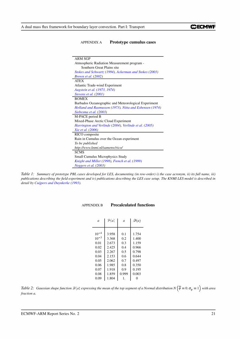
APPENDIX A Prototype cumulus cases

ARM SGPAtmospheric Radiation Measurement program -

Southern Great Plains siteStokes and Schwartz (1994), Ackerman and Stokes (2003)Brown et al. (2002)ATEXAtlantic Trade-wind ExperimentAugstein et al. (1973, 1974)Stevens et al. (2001)BOMEXBarbados Oceanographic and Meteorological ExperimentHolland and Rasmusson (1973), Nitta and Esbensen (1974)Siebesma et al. (2003)M-PACE period BMixed-Phase Arctic Cloud ExperimentHarrington and Verlinde (2004), Verlinde et al. (2005)Xie et al. (2006)RICO compositeRain in Cumulus over the Ocean experimentTo be publishedhttp://www.knmi.nl/samenw/rico/SCMSSmall Cumulus Microphysics StudyKnight and Miller (1998), French et al. (1999)Neggers et al. (2003)

Table 1: Summary of prototype PBL cases developed for LES, documenting (in row-order) i) the case acronym, ii) its full name, iii)publications describing the field-experiment and iv) publications describing the LES case setup. The KNMI LES model is described indetail by Cuijpers and Duynkerke (1993).

APPENDIX B Precalculated functions

a ?A@ a B a ?A@ a B10 C 4 3.958 0.1 1.75410 C 3 3.368 0.2 1.4000.01 2.673 0.3 1.1590.02 2.425 0.4 0.9660.03 2.267 0.5 0.7980.04 2.153 0.6 0.6440.05 2.062 0.7 0.4970.06 1.985 0.8 0.3500.07 1.918 0.9 0.1950.08 1.859 0.999 0.0030.09 1.804 1. 0

Table 2: Gaussian shape function ?A@ a B expressing the mean of the top segment of a Normal distribution N D φ E 0 F σφ E 1 G with areafraction a.



References

Ackerman, T. P., and G. M. Stokes, 2003: The Atmospheric Radiation Measurement program. Phys. Today, 56,38-44.

Albrecht, B. A., A. K. Betts, W. H. Schubert and S. K. Cox, 1979: A model of the thermodynamic structure ofthe Trade-wind boundary layer. Part I: Theoretical formulation and sensitivity tests. J. Atmos. Sci., 36, 73-89.

Augstein, E., H. Riehl, F. Ostapoff and V. Wagner, 1973: Mass and energy transports in an undistrubed Atlantictrade-wind flow. Mon. Wea. Rev., 101, 101-111.

Augstein, E., H. Schmidt and V. Wagner, 1974: The vertical structure of the atmospheric planetary boundarylayer in undistrubed Trade winds over the Atlantic Ocean. Bound.-Layer Meteor., 6, 129-150.

Betts, A. K. and Jakob, C. 2002: Evaluation of the diurnal cycle of precipitation, surface thermody-namics, and surface fluxes in the ECMWF model using LBA data. J. Geophys. Res., 107(D20), doi:10.1029/2001JD000427.

Betts, A. K., 1976: Modeling sub-cloud layer structure and interaction with a shallow cumulus layer. J. Atmos.Sci., 33, 2363-2382.

Bretherton, C. S., J. R. McCaa and H. Grenier, 2004: A new parameterization for shallow cumulus convectionand its application to marine subtropical cloud-topped boundary layers. Part I: Description and 1D results.Mon. Wea. Rev., 132, 864-882.

Brown, A. R., and Co-authors, 2002: Large-eddy simulation of the diurnal cycle of shallow cumulus convectionover land. Quart. J. Roy. Met. Soc., 128, 1075-1094.

Cheinet, S., A. Beljaars, M. Kohler, J.-J. Morcrette, and P. Viterbo, 2004: Assessing physical processes in theECMWF model forecasts through the ARM SGP site measurements. ECMWF Technical Memorandum No.?,October 2004

Cuijpers, J. W. M., and P. G. Duynkerke, 1993: Large-eddy simulation of trade-wind cumulus clouds. J. Atmos.Sci., 50, 3894-3908.

Derbyshire, S. H., and Co-authors, 2004: Sensitivity of moist convection to environmental humidity. Q. J. Roy.Met. Soc., 130, 3055-3079.

Donner, L. J., 1993: A cumulus parameterization including mass fluxes, vertical momentum dynamics, andmesoscale effects. J. Atmos. Sci., 50, 889-906.

Ertel, H., 1942: Der vertikale Turbulenz-Warmestrom in der Atmospahre. Meteor. Z., 59, 1690-1698.

French, J. R., G. Vali and R. D. Kelly, 1999: Evolution of small cumulus clouds in Florida: observations ofpulsating growth. Atmospheric Research, 52, 143-165.

Golaz, J.-C., V. E. Larson and W. R. Cotton, 2002: A PDF-based model for boundary layer clouds. Part I:method and model description. J. Atmos. Sci., 59, 3540-3551.

Grant, A. L. M., 2001: Cloud-base fluxes in the cumulus-capped boundary layer. Quart. J. Roy. Met. Soc., 127,407-421.

Grant, A. L. M., 2006: The cumulus-capped boundary layer. II:Interface fluxes. Quart. J. Roy. Met. Soc., 132,1405-1422.



Harrington, J., and J. Verlinde, 2004: Mixed-phase Arctic Clouds Experiment (M-PACE): The ARM scientificoverview document. Report, U.S. Dep. of Energy, Washington, D. C., 20 pp.

Holland, J. Z., and E. M. Rasmusson, 1973: Measurement of atmospheric mass, energy and momentum budgetsover a 500-kilometer square of tropical ocean. Mon. Wea. Rev., 101, 44-55.

Holtslag, A. A. M., and C.-H. Moeng, 1991: Eddy diffusivity and countergradient transport in the convectiveatmospheric boundary layer. J. Atmos. Sci., 48, 1690-1698.

Kain, J. S. and J. M. Fritsch, 1990: A one-dimensional entraining/detraining plume model and its applicationin convective parameterizations. J. Atmos. Sci., 47, 2784-2802.

Klein, S. A., and D. L. Hartmann, 1993: The seasonal cycle of low stratiform clouds. J. Clim., 6, 1587-1606.

Kohler, M., 2005: Improved prediction of boundary layer clouds. ECMWF Newsletter, No. 104, 18-22.

Knight, C. A. and L. J. Miller, 1998: Early radar echoes from small, warm cumulus: Bragg and hydrometeorscattering. J. Atmos. Sci., 55, 2974-2992.

Lappen, C.-L., and D. A. Randall, 2001: Toward a unified parameterization of the boundary layer and moistconvection. Part I: A new type of mass-flux model. J. Atmos. Sci., 58, 2021-2036.

Larson, V. E., R. Wood, P. R. Field, J.-C. Golaz, T. H. Vonder Haar, and W. R. Cotton, 2001: Small-scale andmesoscale variability of scalars in cloudy boundary layers: One-dimensional probability density functions.J. Atmos. Sci., 58, 1978-1994.

LeMone, M. A., and Pennell, W. T., 1976: The relationship of Trade wind cumulus distribution to subcloudlayer fluxes and structure. Mon. Wea. Rev., 104, 524-539.

Lewellen, W. S., and S. Yoh, 1993: Binormal model of ensemble partial cloudiness. J. Atmos. Sci., 50, 1228-1237.

Lock, A. P., A. R. Brown, M. R. Bush, G. M. Martin, and R. N. B. Smith, 2000: A new boundary layer mixingscheme. Part I: Scheme description and single-column model tests. Mon. Wea. Rev., 128, 3187-3199.

Mace, G. G., C. Jakob, and K. P. Moran, 1998: Validation of hydrometeor occurrence predicted by the ECMWFmodel using millimeter wave radar data. Geophys. Res. Letters, 25, 1645-1648.

Mapes, B. E., 2000: Convective inhibition, subgrid-scale triggering energy, and stratiform instability in a toytropical wave model. J. Atmos. Sci., 57, 1515-1535

Neggers, R. A. J., A. P. Siebesma and H. J. J. Jonker, 2002: A multi parcel model for shallow cumulus convec-tion. J. Atmos. Sci., 59, 1655-1668.

Neggers, R. A. J., P. G. Duynkerke, S. M. A. Rodts, 2003: Shallow cumulus convection: a validation of large-eddy simulation against aircraft and Landsat observations. Q. J. Roy. Met. Soc., 129, p2671-2696.

Neggers, R. A. J., A. P. Siebesma, G. Lenderink and A. A. M. Holtslag. 2004: An evaluation of mass fluxclosures for diurnal cycles of shallow cumulus. Mon. Wea. Rev., 132, p2525-2538.

Neggers, R. A. J., B. Stevens, and J. D. Neelin, 2006a: A simple equilibrium model for shallow cumulus toppedmixed layers. Theoret. Comput. Fluid Dynamics, 20, 305-322. DOI 10.1007/s00162-006-0030-1.

Neggers, R. A. J., B. Stevens, and J. D. Neelin, 2007: Variance scaling in shallow cumulus topped mixed layers.Accepted for publication in the Q. J. Roy. Met. Soc, February 2007.



Nicholls, S., and M. A. LeMone, 1980: The fair weather boundary layer in GATE: the relationship of subcloudfluxes and structure to the distribution and enhancement of cumulus clouds. J. Atmos. Sci., 37, 2051-2067.

Nitta, T. and S. Esbensen, 1974: Heat and moisture budget analyses using BOMEX data. Mon. Wea. Rev., 102,17-28.

Raymond, D. J., and A. M. Blyth, 1986: A stochastic mixing model for non-precipitating cumulus clouds. J.Atmos. Sci., 43, 2708-2718.

Rooy, W. C. de, and A. P. Siebesma, 2006: A simple parameterization for detrainment in shallow cumulus. 17thSymposium on Boundary Layers and Turbulence, 22/5/2006-26/5/2006, San Diego, AMS (int.).

Schumann, U., and C.-H. Moeng, 1991: Plume budgets in clear and cloudy convective boundary layers. J.Atmos. Sci., 48, 1758-1770.

Siebesma, A. P., and J. W. M. Cuijpers, 1995: Evaluation of parametric assumptions for shallow cumulusconvection. J. Atmos. Sci., 52, 650-666.

Siebesma, A. P., 1998: Shallow cumulus convection. Buoyant Convection in Geophysical Flows, E. J. Plate, E.E. Fedorovich, D. X. Viegas and J. C. Wyngaard, Eds., Kluwer Academic Publishers, 441-486.

Siebesma, A. P., and Co-authors, 2003: A large eddy simulation intercomparison study of shallow cumulusconvection. J. Atmos.Sci., 60, 1201-1219.

Siebesma, A. P., and J. Teixeira, 2000: An advection-diffusion scheme for the convective boundary layer:description and 1D-results. Proceedings of the 14th Symposium on Boundary Layer and Turbulence of theAmerican Meteorological Society, 133-140.

Siebesma, A. P., and Co-authors, 2004: Cloud representation in general-circulation models over the northernPacific Ocean: A EUROCS intercomparison study. Q. J. Roy. Met. Soc., 130, p3245-3267.

Siebesma, A. P., P. M. M. Soares, and J. Teixeira: A combined eddy diffusivity mass flux approach for param-eterizing turbulent transport in the convective boundary layer. Submitted to the J. Atmos. Sci., 2007

Sommeria, G., and J. W. Deardorff, 1977: Subgrid-scale condensation in models of non-precipitating clouds.J. Atmos. Sci., 34, 344-355.

Stevens, B., and Co-authors, 2001: Simulations of Trade-wind cumuli under a strong inversion. J. Atmos. Sci.,58, 1870-1891.

Stevens, B., 2006: Boundary layer concepts for simplified models of tropical dynamics. Theoret. Comput. FluidDynamics, 20, 279-304.

Stokes, G. M., and S. E. Schwartz, 1994: The Atmospheric Radiation Measurement (ARM) program: program-matic background and design of the cloud and radiation test bed. Bull. Amer. Meteor. Soc., 75, 1201-1222.

Tiedtke, M., W. A. Heckley and J. Slingo, 1988: Tropical forecasting at ECMWF: The influence of physicalparameterizations on the mean structure of forecasts and analyses. Quart. J. Roy. Met. Soc., 114, 639-665.

Tiedtke, M., 1989: A comprehensive mass flux scheme for cumulus parameterization in large-scale models.Mon. Wea. Rev., 117, 1779-1800.

Tiedtke, M., 1993: Representation of clouds in large-scale models. Mon. Wea. Rev., 121, 3040-3061.



Tompkins, A., and Co-authors, 2004: Moist physical processes in the IFS: Progress and plans. ECMWF tech-nical memorandum, 452pp.

Turner, 1973: Buoyancy effects in fluids. Cambridge University Press, 367pp.

van Ulden, A. P., and A. P. Siebesma, 1997: A model for strong updrafts in the convective boundary layer. Pro-ceedings of the 12th Symposium on Boundary Layers and Turbulence, Aspen, USA, American MeteorologicalSociety, p257-259.

Verlinde, J., et al., 2005: Overview of the Mixed-Phase Arctic Cloud Experiment (M-PACE). Proceedings ofthe 85th Annual Conference of the Am. Meteorol. Soc., San Diego, Ca..

Wyant, M. C., C. S. Bretherton, H. A. Rand, and D. E. Stevens, 1997: Numerical simulations and a conceptualmodel of the stratocumulus to trade cumulus transition. J. Atmos. Sci., 54, 168-192.

Wyngaard, J. C., and C.-H. Moeng, 1992: Parameterizing turbulent diffusion through the joint probabilitydensity. Bound.-Layer Meteor., 60, 1-13.

Xie, S., S. A. Klein, M. Zhang, J. J. Yio, R. T. Cederwall, and R. McCoy, 2006: Developing large-scaleforcing data for single-column and cloud-resolving models from the Mixed-Phase Arctic Cloud Experiment.J. Geophys. Res., 111, D19104, doi:10.1029/2005JD006950.

Yin, B., and B. A. Albrecht, 2000: Spatial variability of atmospheric boundary layer structure over the easternequatorial Pacific. J. Clim., 13, 1574-1592.
