Download pdf - Experiences Gained during the Development of a Passive

Hindawi Publishing CorporationInternational Journal of Navigation and ObservationVolume 2008, Article ID 807958, 12 pagesdoi:10.1155/2008/807958

Research ArticleExperiences Gained during the Development of a PassiveBSAR with GNSS Transmitters of Opportunity

M. Cherniakov, Rajesh Saini, Michael Antoniou, Rui Zuo, and Eleftherios Plakidis

Microwave Integrated Systems Laboratory (MISL), Department of Electronic, Electrical and Computer Engineering,University of Birmingham, Edgbaston, Birmingham B15 2TT, UK

Correspondence should be addressed to M. Cherniakov, [email protected]

Received 18 February 2008; Accepted 14 May 2008

Recommended by M. Greco

This paper presents an overview of the research conducted at University of Birmingham. It highlights and briefly discusses varioussystems parameters (e.g., resolution, power budget), problems (e.g., interference, heterodyne channel Doppler compensation),and signal processing algorithms (imaging, synchronization) required for successfully obtaining an image. The GLONASS satelliteis used for experiential confirmation of the main results. All these results are presented and briefly discussed.

Copyright © 2008 M. Cherniakov et al. This is an open access article distributed under the Creative Commons Attribution License,which permits unrestricted use, distribution, and reproduction in any medium, provided the original work is properly cited.

1. INTRODUCTION

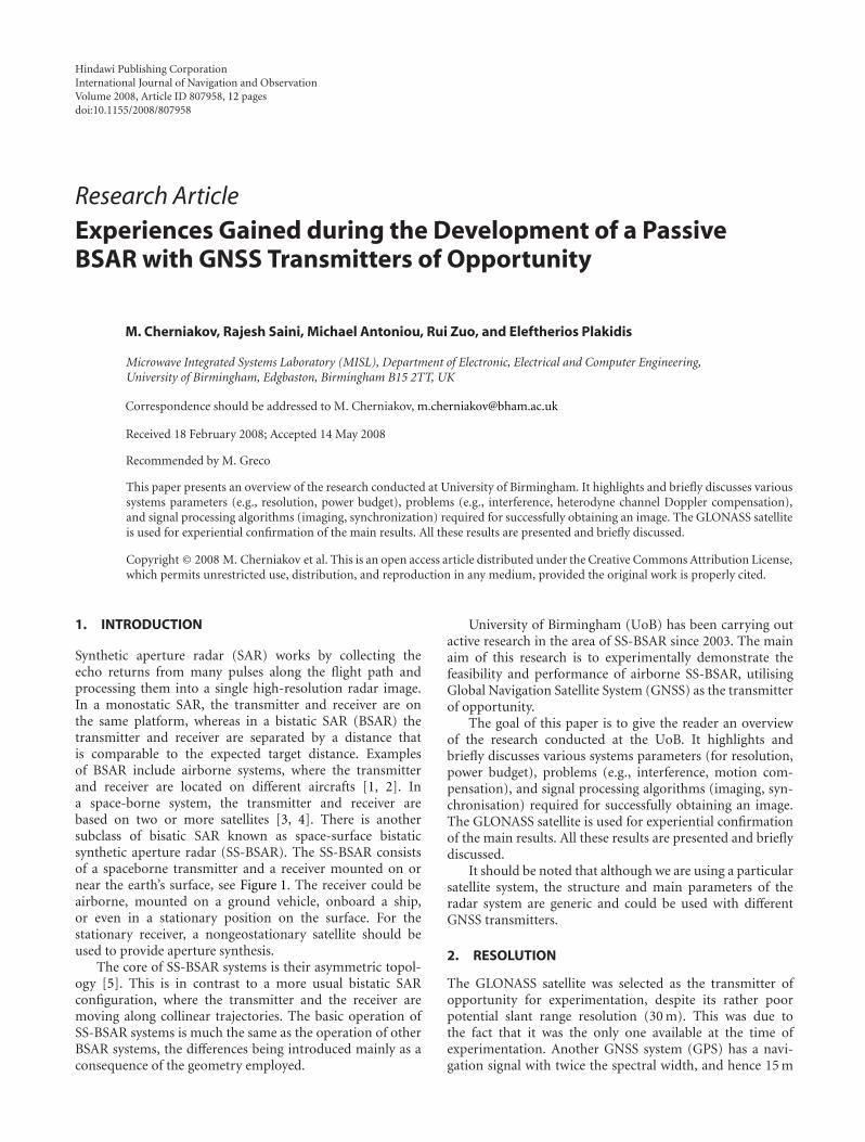
Synthetic aperture radar (SAR) works by collecting theecho returns from many pulses along the flight path andprocessing them into a single high-resolution radar image.In a monostatic SAR, the transmitter and receiver are onthe same platform, whereas in a bistatic SAR (BSAR) thetransmitter and receiver are separated by a distance thatis comparable to the expected target distance. Examplesof BSAR include airborne systems, where the transmitterand receiver are located on different aircrafts [1, 2]. Ina space-borne system, the transmitter and receiver arebased on two or more satellites [3, 4]. There is anothersubclass of bisatic SAR known as space-surface bistaticsynthetic aperture radar (SS-BSAR). The SS-BSAR consistsof a spaceborne transmitter and a receiver mounted on ornear the earth’s surface, see Figure 1. The receiver could beairborne, mounted on a ground vehicle, onboard a ship,or even in a stationary position on the surface. For thestationary receiver, a nongeostationary satellite should beused to provide aperture synthesis.

The core of SS-BSAR systems is their asymmetric topol-ogy [5]. This is in contrast to a more usual bistatic SARconfiguration, where the transmitter and the receiver aremoving along collinear trajectories. The basic operation ofSS-BSAR systems is much the same as the operation of otherBSAR systems, the differences being introduced mainly as aconsequence of the geometry employed.

University of Birmingham (UoB) has been carrying outactive research in the area of SS-BSAR since 2003. The mainaim of this research is to experimentally demonstrate thefeasibility and performance of airborne SS-BSAR, utilisingGlobal Navigation Satellite System (GNSS) as the transmitterof opportunity.

The goal of this paper is to give the reader an overviewof the research conducted at the UoB. It highlights andbriefly discusses various systems parameters (for resolution,power budget), problems (e.g., interference, motion com-pensation), and signal processing algorithms (imaging, syn-chronisation) required for successfully obtaining an image.The GLONASS satellite is used for experiential confirmationof the main results. All these results are presented and brieflydiscussed.

It should be noted that although we are using a particularsatellite system, the structure and main parameters of theradar system are generic and could be used with differentGNSS transmitters.

2. RESOLUTION

The GLONASS satellite was selected as the transmitter ofopportunity for experimentation, despite its rather poorpotential slant range resolution (30 m). This was due tothe fact that it was the only one available at the time ofexperimentation. Another GNSS system (GPS) has a navi-gation signal with twice the spectral width, and hence 15 m

mailto:[email protected]

2 International Journal of Navigation and Observation

Table 1: The main parameters of different GNSS signals.

GNSS GLONASS GPS Galileo

Channels (code) L1(P) L2 (P) L1(P/M) L2 (P/M) L5 E5a/b E5 (E5a+E5b)

Central frequency (MHz) 1602–1615 1246–1257 1575.4 1227.6 1176 1191.79 1191.795

Minimum power (dBW) −161 −167−158 (global beam) −154.9 −157 −154−138 (spot beam)

Chip rate (Mcps) 5.11 5.11 10.23/5.11 10.23/5.11 10.23 10.23 10.23

Aggregated bandwidth (MHz) — — 20–30 20–30 — — 20–50

Range resolution (m) 30 30 5–8 5–8 15 15 3–8

Table 2: Potential target detection range for different GNSS signals.

Transmitter λ(cm) Va(m/s) η Ae(m2) Δaz(m) Ts(K)

Galileo E5 25.2

200 0.5 0.5 1 410GPS L5 25.5

GPS spot beam 19

GLONASS L1 18.8

Radar channel

Heterodyne channel

Moving or stationaryspaceborne transmitter

Movingairborne receiver

Moving or stationaryground-based receiver

Figure 1: SS-BSAR concept for imaging.

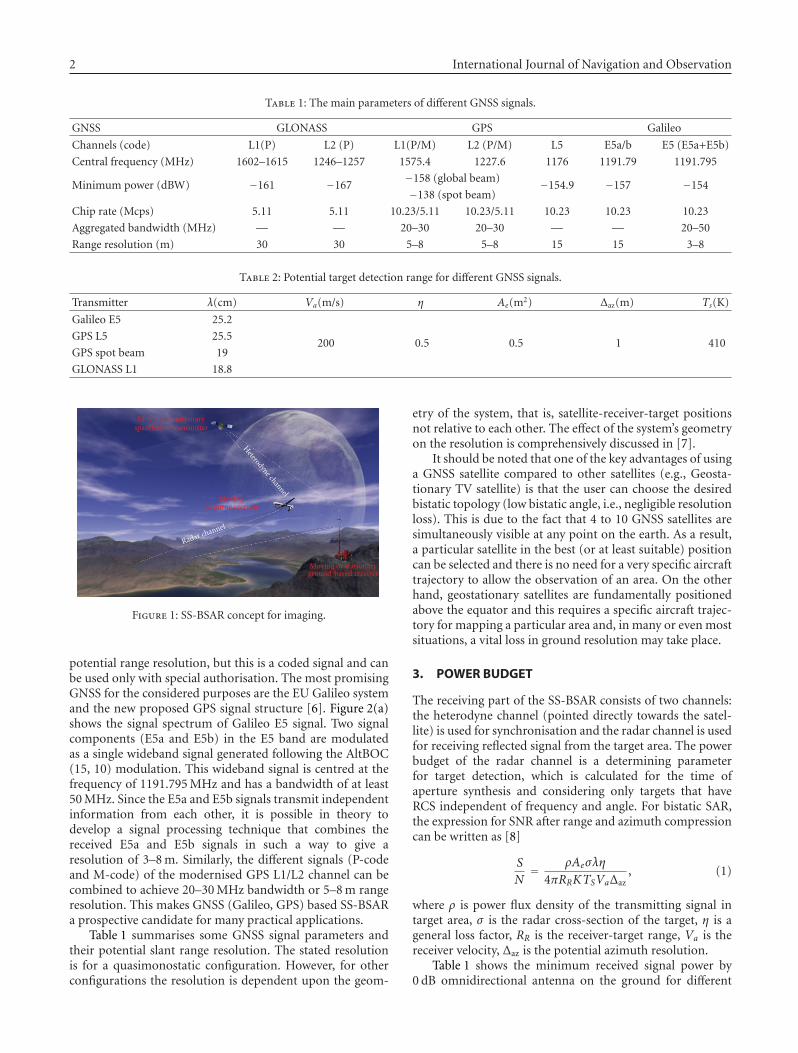
potential range resolution, but this is a coded signal and canbe used only with special authorisation. The most promisingGNSS for the considered purposes are the EU Galileo systemand the new proposed GPS signal structure [6]. Figure 2(a)shows the signal spectrum of Galileo E5 signal. Two signalcomponents (E5a and E5b) in the E5 band are modulatedas a single wideband signal generated following the AltBOC(15, 10) modulation. This wideband signal is centred at thefrequency of 1191.795 MHz and has a bandwidth of at least50 MHz. Since the E5a and E5b signals transmit independentinformation from each other, it is possible in theory todevelop a signal processing technique that combines thereceived E5a and E5b signals in such a way to give aresolution of 3–8 m. Similarly, the different signals (P-codeand M-code) of the modernised GPS L1/L2 channel can becombined to achieve 20–30 MHz bandwidth or 5–8 m rangeresolution. This makes GNSS (Galileo, GPS) based SS-BSARa prospective candidate for many practical applications.

Table 1 summarises some GNSS signal parameters andtheir potential slant range resolution. The stated resolutionis for a quasimonostatic configuration. However, for otherconfigurations the resolution is dependent upon the geom-

etry of the system, that is, satellite-receiver-target positionsnot relative to each other. The effect of the system’s geometryon the resolution is comprehensively discussed in [7].

It should be noted that one of the key advantages of usinga GNSS satellite compared to other satellites (e.g., Geosta-tionary TV satellite) is that the user can choose the desiredbistatic topology (low bistatic angle, i.e., negligible resolutionloss). This is due to the fact that 4 to 10 GNSS satellites aresimultaneously visible at any point on the earth. As a result,a particular satellite in the best (or at least suitable) positioncan be selected and there is no need for a very specific aircrafttrajectory to allow the observation of an area. On the otherhand, geostationary satellites are fundamentally positionedabove the equator and this requires a specific aircraft trajec-tory for mapping a particular area and, in many or even mostsituations, a vital loss in ground resolution may take place.

3. POWER BUDGET

The receiving part of the SS-BSAR consists of two channels:the heterodyne channel (pointed directly towards the satel-lite) is used for synchronisation and the radar channel is usedfor receiving reflected signal from the target area. The powerbudget of the radar channel is a determining parameterfor target detection, which is calculated for the time ofaperture synthesis and considering only targets that haveRCS independent of frequency and angle. For bistatic SAR,the expression for SNR after range and azimuth compressioncan be written as [8]

S

N= ρAeσλη

4πRRKTSVaΔaz, (1)

where ρ is power flux density of the transmitting signal intarget area, σ is the radar cross-section of the target, η is ageneral loss factor, RR is the receiver-target range, Va is thereceiver velocity, Δaz is the potential azimuth resolution.

Table 1 shows the minimum received signal power by0 dB omnidirectional antenna on the ground for different

M. Cherniakov et al. 3

5

0

−5

−10

−15

−20

−25

−30

−35

−40

−45

Am

plit

ude

(dB

W)

−30 −20 −10 0 10 20 30

Frequency (MHz)

(a)

10

5

0

−5

−10

−15

−20

−25

−30

−35

−40

Am

plit

ude

(dB

W)

−20 −15 −10 −5 0 5 10 15 20

Frequency (MHz)

P-codeM-code

(b)

Figure 2: (a) Galileo E5 channel Spectrum, (b) GPS L1 or L2 channel Spectrum.

40

35

30

25

20

15

10

5

0

−5

Sign

al-t

o-n

oise

rati

o(d

B)

0 10 20 30 40 50

Target detection range (km)

Galileo E5GPS L5

GPS spot beamGLONASS L1

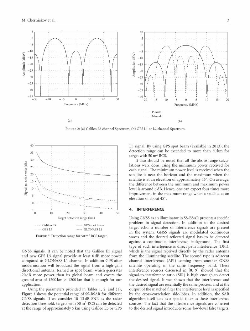
Figure 3: Detection range for 50 m2 RCS target.

GNSS signals. It can be noted that the Galileo E5 signaland new GPS L5 signal provide at least 6 dB more powercompared to GLONASS L1 channel. In addition GPS aftermodernisation will broadcast the signal from a high-gaindirectional antenna, termed as spot beam, which generates20 dB more power than its global beam and covers theground area of 1200 km × 1200 km that is enough for ourapplication.

Using the parameters provided in Tables 1, 2, and (1),Figure 3 shows the potential range of SS-BSAR for differentGNSS signals. If we consider 10–13 dB SNR as the radardetection threshold, targets with 50 m2 RCS can be detectedat the range of approximately 5 km using Galileo E5 or GPS

L5 signal. By using GPS spot beam (available in 2013), thedetection range can be extended to more than 50 km fortarget with 50 m2 RCS.

It also should be noted that all the above range calcu-lations were done using the minimum power received foreach signal. The minimum power level is received when thesatellite is near the horizon and the maximum when thesatellite is at an elevation of approximately 45◦. On average,the difference between the minimum and maximum powerlevel is around 6 dB. Hence, one can expect four times moreimprovement in the maximum range when a satellite at anelevation of about 45◦.

4. INTERFERENCE

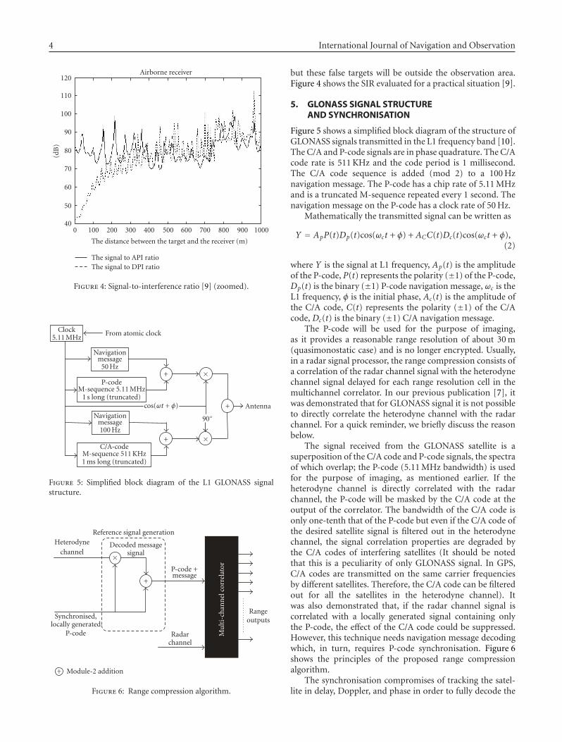
Using GNSS as an illuminator in SS-BSAR presents a specificproblem in signal detection. In addition to the desiredtarget echo, a number of interference signals are presentin the system. GNSS signals are modulated continuouswaves and the desired reflected signal has to be detectedagainst a continuous interference background. The firsttype of such interference is direct path interference (DPI),which is the signal received directly by the radar antennafrom the illuminating satellite. The second type is adjacentchannel interference (API) coming from another GNSSsatellite operating in the same frequency band. Theseinterference sources discussed in [8, 9] showed that thesignal-to-interference ratio (SIR) is high enough to detectthe desired signal. It was shown that the interference andthe desired signal are essentially the same process, and at theoutput of the matched filter the interference level is specifiedby the cross-correlation side-lobes. In addition, the SARalgorithm itself acts as a spatial filter to these interferencesources. The fact that the interference signals are coherentto the desired signal introduces some low-level false targets,


Airborne receiver120

110

100

90

80

70

60

50

40

(dB

)

0 100 200 300 400 500 600 700 800 900 1000

The distance between the target and the receiver (m)

The signal to API ratioThe signal to DPI ratio

Figure 4: Signal-to-interference ratio [9] (zoomed).

Clock5.11 MHz

+ ×

+

+ ×

Antenna

P-codeM-sequence 5.11 MHz

1 s long (truncated)

From atomic clock

Navigationmessage

50 Hz

Navigationmessage100 Hz

C/A-codeM-sequence 511 KHz1 ms long (truncated)

90◦cos(ωt + φ)

Figure 5: Simplified block diagram of the L1 GLONASS signalstructure.

+

+ Module-2 addition

×

Mu

lti-

chan

nel

corr

elat

or

Radarchannel

Reference signal generation

Decoded messagesignal

Heterodynechannel

Synchronised,locally generated

P-code

P-code +message

Rangeoutputs

Figure 6: Range compression algorithm.

but these false targets will be outside the observation area.Figure 4 shows the SIR evaluated for a practical situation [9].

5. GLONASS SIGNAL STRUCTUREAND SYNCHRONISATION

Figure 5 shows a simplified block diagram of the structure ofGLONASS signals transmitted in the L1 frequency band [10].The C/A and P-code signals are in phase quadrature. The C/Acode rate is 511 KHz and the code period is 1 millisecond.The C/A code sequence is added (mod 2) to a 100 Hznavigation message. The P-code has a chip rate of 5.11 MHzand is a truncated M-sequence repeated every 1 second. Thenavigation message on the P-code has a clock rate of 50 Hz.

Mathematically the transmitted signal can be written as

Y = ApP(t)Dp(t)cos(ωct + φ) + ACC(t)Dc(t)cos(ωct + φ),(2)

where Y is the signal at L1 frequency, Ap(t) is the amplitudeof the P-code, P(t) represents the polarity (±1) of the P-code,Dp(t) is the binary (±1) P-code navigation message, ωc is theL1 frequency, φ is the initial phase, Ac(t) is the amplitude ofthe C/A code, C(t) represents the polarity (±1) of the C/Acode, Dc(t) is the binary (±1) C/A navigation message.

The P-code will be used for the purpose of imaging,as it provides a reasonable range resolution of about 30 m(quasimonostatic case) and is no longer encrypted. Usually,in a radar signal processor, the range compression consists ofa correlation of the radar channel signal with the heterodynechannel signal delayed for each range resolution cell in themultichannel correlator. In our previous publication [7], itwas demonstrated that for GLONASS signal it is not possibleto directly correlate the heterodyne channel with the radarchannel. For a quick reminder, we briefly discuss the reasonbelow.

The signal received from the GLONASS satellite is asuperposition of the C/A code and P-code signals, the spectraof which overlap; the P-code (5.11 MHz bandwidth) is usedfor the purpose of imaging, as mentioned earlier. If theheterodyne channel is directly correlated with the radarchannel, the P-code will be masked by the C/A code at theoutput of the correlator. The bandwidth of the C/A code isonly one-tenth that of the P-code but even if the C/A code ofthe desired satellite signal is filtered out in the heterodynechannel, the signal correlation properties are degraded bythe C/A codes of interfering satellites (It should be notedthat this is a peculiarity of only GLONASS signal. In GPS,C/A codes are transmitted on the same carrier frequenciesby different satellites. Therefore, the C/A code can be filteredout for all the satellites in the heterodyne channel). Itwas also demonstrated that, if the radar channel signal iscorrelated with a locally generated signal containing onlythe P-code, the effect of the C/A code could be suppressed.However, this technique needs navigation message decodingwhich, in turn, requires P-code synchronisation. Figure 6shows the principles of the proposed range compressionalgorithm.

The synchronisation compromises of tracking the satel-lite in delay, Doppler, and phase in order to fully decode the


SC

HC

RC

Three channelmicrowave receiver

Satellite 1 Satellite 4

HC

3 m

RC

Cables (25 m)Control room

Splitter

GNSS receiver(supplied by topcon)

Computer

IF1 (1.53 GHz) IF2 (70 MHz)

Dataacquisition

IHC

QHC

IRC

QRC

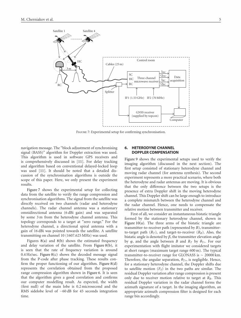
Figure 7: Experimental setup for confirming synchronisation.

navigation message. The “block adjustment of synchronisingsignal (BASS)” algorithm for Doppler extraction was used.This algorithm is used in software GPS receivers andis comprehensively discussed in [11]. For delay trackingand algorithm based on conventional delayed-locked loopwas used [11]. It should be noted that a detailed dis-cussion of the synchronisation algorithms is outside thescope of this paper. Here, we only present the experimentresults.

Figure 7 shows the experimental setup for collectingdata from the satellite to verify the range compression andsynchronisation algorithms. The signal from the satellite wasdirectly received on two channels (radar and heterodynechannels). The radar channel antenna was a stationaryomnidirectional antenna (6 dBi gain) and was separatedby some 3 m from the heterodyne channel antenna. Thistopology corresponds to a target at “zero range.” For theheterodyne channel, a directional spiral antenna with again of 16 dBi was pointed towards the satellite. A satellitetransmitting on channel 10 (1607.625 MHz) was used.

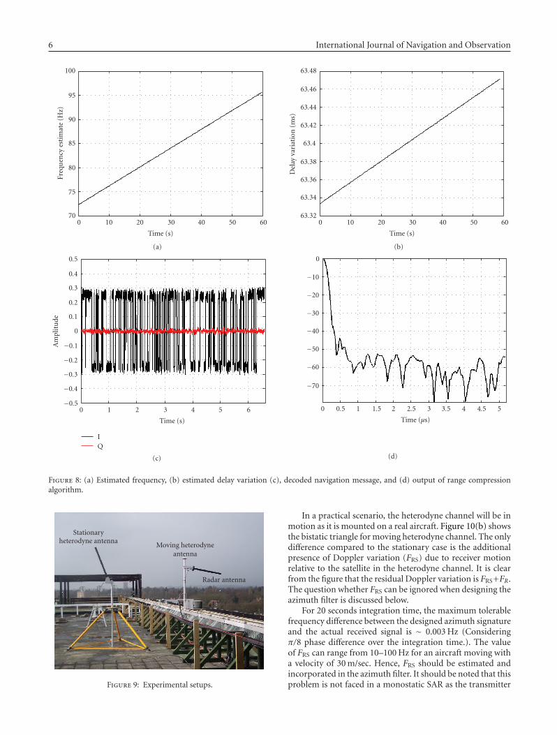
Figures 8(a) and 8(b) shows the estimated frequencyand delay variation of the satellite. From Figure 8(b), itis seen that the rate of frequency variation is around0.4 Hz/sec. Figure 8(c) shows the decoded message signalfrom the P-code after phase tracking. These results con-firm the proper functioning of our algorithm. Figure 8(d)represents the correlation obtained from the proposedrange compression algorithm shown in Figure 6. It is seenthat the algorithm gives a good correlation and confirmsour computer modelling result. As expected, the width(first null) of the main lobe is 0.2 microsecond and theRMS sidelobe level of −60 dB for 45 seconds integrationtime.

6. HETERODYNE CHANNELDOPPLER COMPENSATION

Figure 9 shows the experimental setups used to verify theimaging algorithm (discussed in the next section). Thefirst setup consisted of stationary heterodyne channel andmoving radar channel (for antenna synthesis). The secondexperiment represents a more practical scenario, where boththe heterodyne and radar antennas are moving. It is obviousthat the only difference between the two setups is thepresence of extra Doppler shift in the moving heterodynechannel. This Doppler shift can be large enough to introducea complete mismatch between the heterodyne channel andthe radar channel. Hence, one needs to compensate therelative motion between transmitter and receiver.

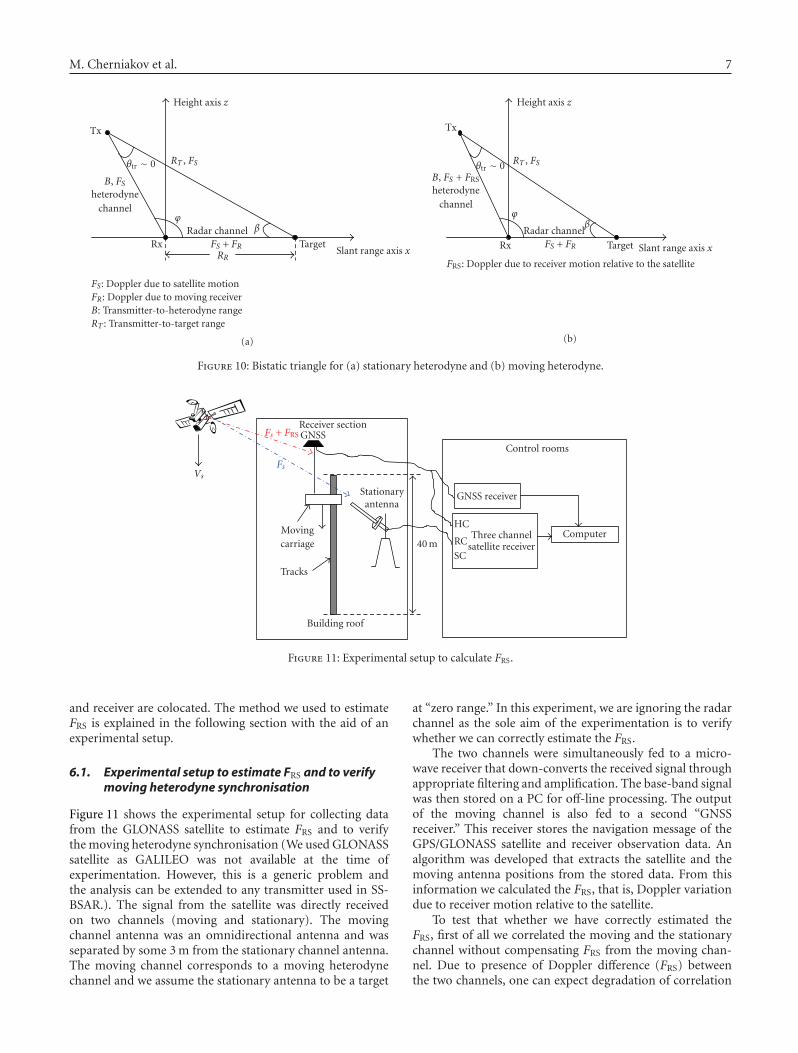
First of all, we consider an instantaneous bistatic triangleformed by the stationary heterodyne channel, shown inFigure 10(a). The three arms of the bistatic triangle aretransmitter-to-receiver path (represented by B), transmitter-to-target path (RT), and target-to-receiver (RR). Also, thebistatic angle is denoted by β, the transmitter elevation angleby ϕ, and the angle between B and RT by θTr . For ourexperimentation with flight imitator we considered targetsat short ranges (maximum target range 600 m). The typicaltransmitter-to-receiver range for GLONASS is ∼ 20000 km.Therefore, the angular separation, θTr , is negligible. Hence,for a stationary heterodyne channel, the Doppler shifts dueto satellite motion (FS) in the two paths are similar. Theresidual Doppler variation after range compression is presentonly due to receiver motion relative to target at RR. Thisresidual Doppler variation in the radar channel forms theazimuth signature of a target. In the imaging algorithm, anappropriate azimuth compression filter is designed for eachrange bin accordingly.


100

95

90

85

80

75

70

Freq

uen

cyes

tim

ate

(Hz)

0 10 20 30 40 50 60

Time (s)

(a)

63.48

63.46

63.44

63.42

63.4

63.38

63.36

63.34

63.32

Del

ayva

riat

ion

(ms)

0 10 20 30 40 50 60

Time (s)

(b)

0.5

0.4

0.3

0.2

0.1

0

−0.1

−0.2

−0.3

−0.4

−0.5

Am

plit

ude

0 1 2 3 4 5 6

Time (s)

IQ

(c)

0

−10

−20

−30

−40

−50

−60

−70

0 0.5 1 1.5 2 2.5 3 3.5 4 4.5 5

Time (μs)

(d)

Figure 8: (a) Estimated frequency, (b) estimated delay variation (c), decoded navigation message, and (d) output of range compressionalgorithm.

Stationaryheterodyne antenna

Moving heterodyneantenna

Radar antenna

Figure 9: Experimental setups.

In a practical scenario, the heterodyne channel will be inmotion as it is mounted on a real aircraft. Figure 10(b) showsthe bistatic triangle for moving heterodyne channel. The onlydifference compared to the stationary case is the additionalpresence of Doppler variation (FRS) due to receiver motionrelative to the satellite in the heterodyne channel. It is clearfrom the figure that the residual Doppler variation is FRS+FR.The question whether FRS can be ignored when designing theazimuth filter is discussed below.

For 20 seconds integration time, the maximum tolerablefrequency difference between the designed azimuth signatureand the actual received signal is ∼ 0.003 Hz (Consideringπ/8 phase difference over the integration time.). The valueof FRS can range from 10–100 Hz for an aircraft moving witha velocity of 30 m/sec. Hence, FRS should be estimated andincorporated in the azimuth filter. It should be noted that thisproblem is not faced in a monostatic SAR as the transmitter


Height axis z

Tx

B, FSheterodyne

channel

RT , FSθtr ∼ 0

ϕβRadar channel

FS + FRRR

Rx TargetSlant range axis x

FS: Doppler due to satellite motionFR: Doppler due to moving receiverB: Transmitter-to-heterodyne rangeRT : Transmitter-to-target range

(a)

Height axis z

Tx

B, FS + FRS

heterodynechannel

RT , FSθtr ∼ 0

ϕβ

Radar channelFS + FRRx Target Slant range axis x

FRS: Doppler due to receiver motion relative to the satellite

(b)

Figure 10: Bistatic triangle for (a) stationary heterodyne and (b) moving heterodyne.

SC

HC

RCThree channel

satellite receiver40 m

Vs

Control rooms

GNSS receiver

Computer

Building roof

Stationaryantenna

Movingcarriage

Tracks

Receiver sectionGNSS

Fs

Fs + FRS

Figure 11: Experimental setup to calculate FRS.

and receiver are colocated. The method we used to estimateFRS is explained in the following section with the aid of anexperimental setup.

6.1. Experimental setup to estimate FRS and to verifymoving heterodyne synchronisation

Figure 11 shows the experimental setup for collecting datafrom the GLONASS satellite to estimate FRS and to verifythe moving heterodyne synchronisation (We used GLONASSsatellite as GALILEO was not available at the time ofexperimentation. However, this is a generic problem andthe analysis can be extended to any transmitter used in SS-BSAR.). The signal from the satellite was directly receivedon two channels (moving and stationary). The movingchannel antenna was an omnidirectional antenna and wasseparated by some 3 m from the stationary channel antenna.The moving channel corresponds to a moving heterodynechannel and we assume the stationary antenna to be a target

at “zero range.” In this experiment, we are ignoring the radarchannel as the sole aim of the experimentation is to verifywhether we can correctly estimate the FRS.

The two channels were simultaneously fed to a micro-wave receiver that down-converts the received signal throughappropriate filtering and amplification. The base-band signalwas then stored on a PC for off-line processing. The outputof the moving channel is also fed to a second “GNSSreceiver.” This receiver stores the navigation message of theGPS/GLONASS satellite and receiver observation data. Analgorithm was developed that extracts the satellite and themoving antenna positions from the stored data. From thisinformation we calculated the FRS, that is, Doppler variationdue to receiver motion relative to the satellite.

To test that whether we have correctly estimated theFRS, first of all we correlated the moving and the stationarychannel without compensating FRS from the moving chan-nel. Due to presence of Doppler difference (FRS) betweenthe two channels, one can expect degradation of correlation


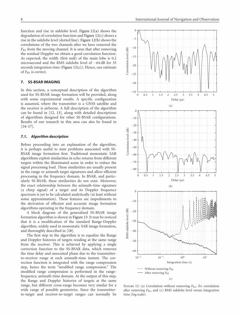
function and rise in sidelobe level. Figure 12(a) shows thedegradation of correlation function and Figure 12(c) shows arise in the sidelobe level (dotted line). Figure 12(b) shows thecorrelations of the two channels after we have removed theFRS from the moving channel. It is seen that after removingthe residual Doppler we obtain a good correlation function.As expected, the width (first null) of the main lobe is 0.2microsecond and the RMS sidelobe level of −64 dB for 35seconds integration time (Figure 12(c)). Hence, our estimateof FRS is correct.

7. SS-BSAR IMAGING

In this section, a conceptual description of the algorithmused for SS-BSAR image formation will be provided, alongwith some experimental results. A specific configurationis assumed, where the transmitter is a GNSS satellite andthe receiver is airborne. A full description of the algorithmcan be found in [12, 13], along with detailed descriptionsof algorithms designed for other SS-BSAR configurations.Results of our research in this area can also be found in[14–17].

7.1. Algorithm description

Before proceeding into an explanation of the algorithm,it is perhaps useful to state problems associated with SS-BSAR image formation first. Traditional monostatic SARalgorithms exploit similarities in echo returns from differenttargets within the illuminated scene in order to reduce thesignal processing load. These similarities are usually presentin the range or azimuth target signatures and allow efficientprocessing in the frequency domain. In BSAR, and partic-ularly SS-BSAR, these similarities do not exist. Moreover,the exact relationship between the azimuth-time signature(a chirp signal) of a target and its Doppler frequencyspectrum is yet to be calculated analytically (at least withoutsome approximation). These features are impediments tothe derivation of efficient and accurate image formationalgorithms operating in the frequency domain.

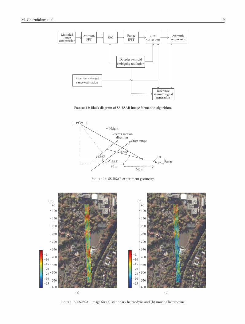
A block diagram of the generalised SS-BSAR imageformation algorithm is shown in Figure 13. It may be noticedthat it is a modification of the standard Range-Doppleralgorithm, widely used in monostatic SAR image formation,and thoroughly described in [18].

The first step in the algorithm is to equalize the Rangeand Doppler histories of targets residing at the same rangefrom the receiver. This is achieved by applying a singlecorrection function to the SS-BSAR data, which removesthe time delay and associated phase due to the transmitter-to-receiver range at each azimuth-time instant. The cor-rection function is integrated with the range compressionstep, hence the term “modified range compression.” Themodified range compression is performed in the range-frequency, azimuth-time domain. At the output of this step,the Range and Doppler histories of targets at the samerange, but different cross-range becomes very similar for awide range of possible geometries. Since the transmitter-to-target and receiver-to-target ranges can normally be

0

−5

−10

−15

−20

−25

−30

−35

Cor

rela

tion

leve

l(dB

)

0 0.5 1 1.5 2 2.5 3 3.5 4 4.5 5

Delay (μs)

(a)

0

−10

−20

−30

−40

−50

−60

−70

−80

Cor

rela

tion

leve

l(dB

)

0 0.5 1 1.5 2 2.5 3 3.5 4 4.5 5

Delay (μs)

(b)

0

−10

−20

−30

−40

−50

−60

RM

Ssi

delo

bele

vel(

dB)

10−2 10−1 100 101

Integration time (s)

Without removing FRS

After removing FRS

(c)

Figure 12: (a) Correlation without removing FRS, (b) correlationafter removing FRS, and (c) RMS sidelobe level versus integrationtime (log scale).


Modifiedrange

compression

AzimuthFFT

SRCRangeIFFT

RCMcorrection

Azimuthcompression

Doppler centroidambiguity resolution

Receiver-to-targetrange estimation

Referenceazimuth signal

generation

Figure 13: Block diagram of SS-BSAR image formation algorithm.

Height

Receiver motiondirection

Cross-range

Range27 m

540 m60 m

11.36◦

178.5◦

5.63◦

Figure 14: SS-BSAR experiment geometry.

−5

−10

−15

−20

−25

−30

−35

60

100

150

200

250

300

350

400

450

500

550

600

(m)

(a)

(m)

−5

−10

−15

−20

−25

−30

−35

60

100

150

200

250

300

350

400

450

500

550

600

(b)

Figure 15: SS-BSAR image for (a) stationary heterodyne and (b) moving heterodyne.


Table 3: Experimental parameters.

Parameter Stationary heterodyne Moving heterodyne

GLONASS satellite COSMOS 2394 COSMOS 2418

Carrier frequency (MHz) 1603.125 1603.125

Signal bandwidth (MHz) 5.11 5.11

Satellite’s azimuth angle (degree) 178.49 182

Satellite’s elevation angle (degree) 11.36 38

Bistatic angle (degree) 5.63 38

Receiver velocity (m/sec) 0.6 0.6

Receiver’s height above the ground (m) ∼25 ∼25

Receiver’s aperture length (m) 27 27

Integration time (s) 45 45

approximated using second-order Taylor series expansionsin SS-BSAR, it is also possible to derive signal expressionsin the frequency domain. Therefore, use of a modificationof the Range-Doppler algorithm is a convenient method toform the image of an observation area. A secondary rangecompression (SRC) is performed in the two-dimensionalfrequency domain to compensate for the cross-couplingbetween the range and azimuth frequencies. Before thisoperation is executed, the Doppler ambiguity is resolved(i.e., because the target azimuth signature could contain alarge Doppler centroid outside the range of sampled azimuthfrequencies). Range cell migration (RCM) is corrected inthe range-time, azimuth-frequency (or Range, Doppler)domain, after RCM components due to the receiver motionand residual RCM after the modified range compressionare calculated. For this operation, it is proposed to esti-mate the receiver-to-target range from the range sum(the difference between the total range history and thetransmitter-to-receiver range history) in order to identifythe individual RCM components mentioned above. Finally,azimuth compression is performed in the range, Dopplerdomain.

7.2. Experimental results

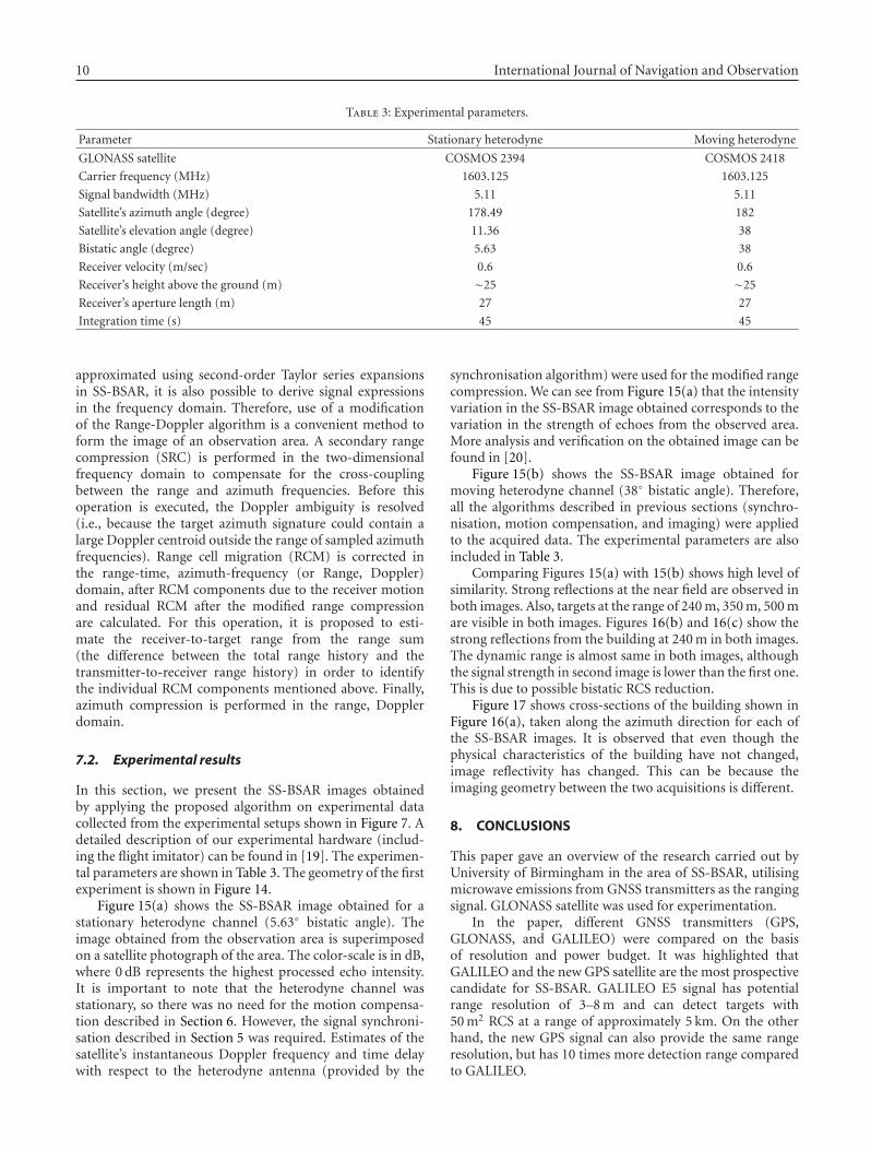
In this section, we present the SS-BSAR images obtainedby applying the proposed algorithm on experimental datacollected from the experimental setups shown in Figure 7. Adetailed description of our experimental hardware (includ-ing the flight imitator) can be found in [19]. The experimen-tal parameters are shown in Table 3. The geometry of the firstexperiment is shown in Figure 14.

Figure 15(a) shows the SS-BSAR image obtained for astationary heterodyne channel (5.63◦ bistatic angle). Theimage obtained from the observation area is superimposedon a satellite photograph of the area. The color-scale is in dB,where 0 dB represents the highest processed echo intensity.It is important to note that the heterodyne channel wasstationary, so there was no need for the motion compensa-tion described in Section 6. However, the signal synchroni-sation described in Section 5 was required. Estimates of thesatellite’s instantaneous Doppler frequency and time delaywith respect to the heterodyne antenna (provided by the

synchronisation algorithm) were used for the modified rangecompression. We can see from Figure 15(a) that the intensityvariation in the SS-BSAR image obtained corresponds to thevariation in the strength of echoes from the observed area.More analysis and verification on the obtained image can befound in [20].

Figure 15(b) shows the SS-BSAR image obtained formoving heterodyne channel (38◦ bistatic angle). Therefore,all the algorithms described in previous sections (synchro-nisation, motion compensation, and imaging) were appliedto the acquired data. The experimental parameters are alsoincluded in Table 3.

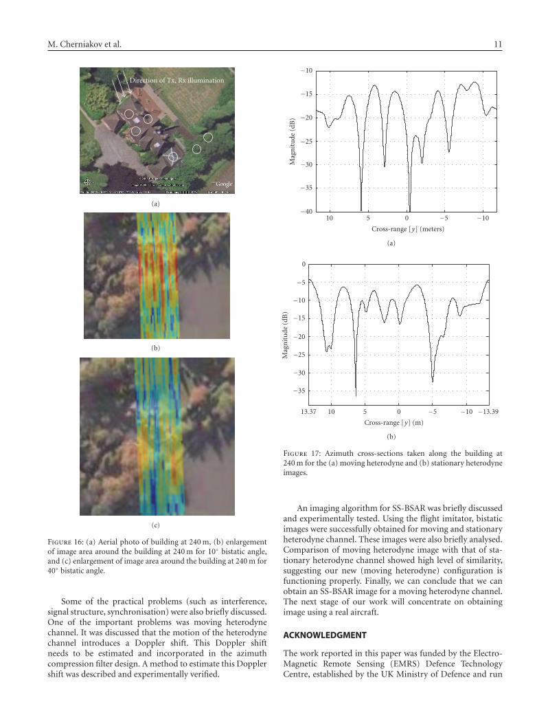
Comparing Figures 15(a) with 15(b) shows high level ofsimilarity. Strong reflections at the near field are observed inboth images. Also, targets at the range of 240 m, 350 m, 500 mare visible in both images. Figures 16(b) and 16(c) show thestrong reflections from the building at 240 m in both images.The dynamic range is almost same in both images, althoughthe signal strength in second image is lower than the first one.This is due to possible bistatic RCS reduction.

Figure 17 shows cross-sections of the building shown inFigure 16(a), taken along the azimuth direction for each ofthe SS-BSAR images. It is observed that even though thephysical characteristics of the building have not changed,image reflectivity has changed. This can be because theimaging geometry between the two acquisitions is different.

8. CONCLUSIONS

This paper gave an overview of the research carried out byUniversity of Birmingham in the area of SS-BSAR, utilisingmicrowave emissions from GNSS transmitters as the rangingsignal. GLONASS satellite was used for experimentation.

In the paper, different GNSS transmitters (GPS,GLONASS, and GALILEO) were compared on the basisof resolution and power budget. It was highlighted thatGALILEO and the new GPS satellite are the most prospectivecandidate for SS-BSAR. GALILEO E5 signal has potentialrange resolution of 3–8 m and can detect targets with50 m2 RCS at a range of approximately 5 km. On the otherhand, the new GPS signal can also provide the same rangeresolution, but has 10 times more detection range comparedto GALILEO.


Direction of Tx, Rx illumination

(a)

(b)

(c)

Figure 16: (a) Aerial photo of building at 240 m, (b) enlargementof image area around the building at 240 m for 10◦ bistatic angle,and (c) enlargement of image area around the building at 240 m for40◦ bistatic angle.

Some of the practical problems (such as interference,signal structure, synchronisation) were also briefly discussed.One of the important problems was moving heterodynechannel. It was discussed that the motion of the heterodynechannel introduces a Doppler shift. This Doppler shiftneeds to be estimated and incorporated in the azimuthcompression filter design. A method to estimate this Dopplershift was described and experimentally verified.

−10

−15

−20

−25

−30

−35

−40

Mag

nit

ude

(dB

)

10 5 0 −5 −10

Cross-range [y] (meters)

(a)

0

−5

−10

−15

−20

−25

−30

−35

Mag

nit

ude

(dB

)

13.37 10 5 0 −5 −10 −13.39

Cross-range [y] (m)

(b)

Figure 17: Azimuth cross-sections taken along the building at240 m for the (a) moving heterodyne and (b) stationary heterodyneimages.

An imaging algorithm for SS-BSAR was briefly discussedand experimentally tested. Using the flight imitator, bistaticimages were successfully obtained for moving and stationaryheterodyne channel. These images were also briefly analysed.Comparison of moving heterodyne image with that of sta-tionary heterodyne channel showed high level of similarity,suggesting our new (moving heterodyne) configuration isfunctioning properly. Finally, we can conclude that we canobtain an SS-BSAR image for a moving heterodyne channel.The next stage of our work will concentrate on obtainingimage using a real aircraft.

ACKNOWLEDGMENT

The work reported in this paper was funded by the Electro-Magnetic Remote Sensing (EMRS) Defence TechnologyCentre, established by the UK Ministry of Defence and run


by a consortium of SELEX Sensors and Airborne Systems,Thales Defence, Roke Manor Research, and Filtronic. Projectno. 1/27.

REFERENCES

[1] P. Dubois-Fernandez, H. Cantalloube, B. Vaizan, et al.,“ONERA-DLR bistatic SAR campaign: planning, data acqui-sition, and first analysis of bistatic scattering behaviour ofnatural and urban targets,” IEE Proceedings: Radar, Sonar andNavigation, vol. 153, no. 3, pp. 214–223, 2006.

[2] I. Walterscheid, J. H. G. Ender, A. R. Brenner, and O. Loffeld,“Bistatic SAR processing and experiments,” IEEE Transactionson Geoscience and Remote Sensing, vol. 44, no. 10, pp. 2710–2717, 2006.

[3] A. Moccia, N. Chiacchio, and A. Capone, “Spaceborne bistaticsynthetic aperture radar for remote sensing applications,”International Journal of Remote Sensing, vol. 21, no. 18, pp.3395–3414, 2000.

[4] M. Younis, R. Metzig, and G. Krieger, “Performance predictionof a phase synchronization link for bistatic SAR,” IEEEGeoscience and Remote Sensing Letters, vol. 3, no. 3, pp. 429–433, 2006.

[5] M. Cherniakov, “Space-surface bistatic synthetic apertureradar—prospective and problems,” in Proceedings of theIEEE International Radar Conference, no. 490, pp. 22–25,Edinburgh, UK, October 2002.

[6] http://www.en.wilkipedia.org/wiki/GPS modernization.[7] M. Cherniakov, R. Saini, M. Antoniou, R. Zuo, and

J. Edwards, “SS-BSAR with transmitter of opportunity—practical aspects,” in Proceedings of the 3rd EMRS DTCTechnical Conference, Edinburgh, UK, July 2006.

[8] X. He, M. Cherniakov, and T. Zeng, “Signal detectabilityin SS-BSAR with GNSS non-cooperative transmitter,” IEEProceedings: Radar, Sonar and Navigation, vol. 152, no. 3, pp.124–132, 2005.

[9] X. He, T. Zeng, and M. Cherniakov, “Interference level eval-uation in SS-BSAR with GNSS non-cooperative transmitter,”Electronics Letters, vol. 40, no. 19, pp. 1222–1224, 2004.

[10] U. Roßbach, Positioning and navigation using the Russiansatellite system GLONASS, Ph.D. thesis, Universitat der Bun-deswehr Munchen, Munchen, Germany, 2000.

[11] J. B.-Y. Tsui, Fundamentals of Global Positioning SystemReceivers: A Software Approach, John Wiley & Sons, New York,NY, USA, 2000.

[12] M. Antoniou, Image formation algorithms for space-surfacebistatic SAR, Ph.D. thesis, University of Birmingham, Birm-ingham, UK, 2007.

[13] M. Antoniou, M. Cherniakov, and C. Hu, “Space-surfaceBSAR image formation algorithms,” submitted to IEEE Trans-actions in Geoscience and Remote Sensing.

[14] M. Cherniakov, M. Antoniou, R. Saini, R. Zuo, and J. Edwards,“Space-surface BSAR—analytical and experimental study,”in Proceedings of the 6th European Conference on SyntheticAperture Radar (EUSAR ’06), Dresden, Germany, May 2006.

[15] M. Antoniou, R. Saini, and M. Cherniakov, “Results of aspace-surface bistatic SAR image formation algorithm,” IEEETransactions on Geoscience and Remote Sensing, vol. 45, no. 11,pp. 3359–3371, 2007.

[16] M. Antoniou, R. Saini, R. Zuo, and M. Cherniakov, “Imageformation algorithm for space-surface BSAR,” in Proceedingsof the 4th European Radar Conference (EuRAD ’07), pp. 413–416, Munich, Germany, October 2007.

[17] M. Antoniou, R. Saini, R. Zuo, and M. Cherniakov, “Space-surface bistatic SAR topology and its impact on imageformation,” in Proceedings of the 7th European Conferenceon Synthetic Aperture Radar (EUSAR ’08), Friedrichshafen,Germany, June 2008.

[18] I. G. Cumming and F. H. Wong, Digital Processing of SyntheticAperture Radar Data: Algorithms and Implementation, ArtechHouse, Norwood, Mass, USA, 2005.

[19] R. Zuo, Test bed development for space-surface bistatic SARinvestigation, M.S. thesis, University of Birmingham, Birming-ham, UK, October 2005.

[20] M. Cherniakov, R. Saini, R. Zuo, and M. Antoniou, “Space-surface bistatic synthetic aperture radar with global naviga-tion satellite system transmitter of opportunity-experimentalresults,” IET Radar, Sonar & Navigation, vol. 1, no. 6, pp. 447–458, 2007.

http://www.en.wilkipedia.org/wiki/GPS_modernization

International Journal of

AerospaceEngineeringHindawi Publishing Corporationhttp://www.hindawi.com Volume 2010

RoboticsJournal of

Hindawi Publishing Corporationhttp://www.hindawi.com Volume 2014


Active and Passive Electronic Components

Control Scienceand Engineering

Journal of



RotatingMachinery


Hindawi Publishing Corporation http://www.hindawi.com

Journal ofEngineeringVolume 2014

Submit your manuscripts athttp://www.hindawi.com

VLSI Design



Shock and Vibration


Civil EngineeringAdvances in

Acoustics and VibrationAdvances in



Electrical and Computer Engineering

Journal of

Advances inOptoElectronics

Hindawi Publishing Corporation http://www.hindawi.com

Volume 2014

The Scientific World JournalHindawi Publishing Corporation http://www.hindawi.com Volume 2014

SensorsJournal of


Modelling & Simulation in EngineeringHindawi Publishing Corporation http://www.hindawi.com Volume 2014


Chemical EngineeringInternational Journal of Antennas and

Propagation




Navigation and Observation



DistributedSensor Networks
