Download pdf - Finding Pattern Configurations for Bank Cheque Printing

Procedia - Social and Behavioral Sciences 108 ( 2014 ) 219 – 234

1877-0428 © 2013 The Authors. Published by Elsevier Ltd. Selection and peer-review under responsibility of AIRO.doi: 10.1016/j.sbspro.2013.12.833

ScienceDirect

Finding Pattern Configurations for Bank Cheque Printing

R. Cerullia,1, R. De Leoneb,2, M. Gentilia,1,3

aDepartment of Mathematics, University of Salerno, Italyb School of Science and Technology, University of Camerino, Italy

Abstract

The problem we address in this paper arises in large-scale manufacturing of bank cheques. Due to security reasons,

the cheques must be printed on special (expensive) paper. The first step in the printing process is to prepare the plates

that will be used by the composing machine. If the imprint (image) of a particular cheque is on a plate, each time

the composing machine uses this plate a new cheque of this type is produced. Each plate has a predefined number of

positions to be impressed. Due to delivery due dates, there is an additional constraint requiring each cheque not to be

present in more than a predefined number of different plates. There are two different production costs that have to be

considered: overproduction costs and printing costs. Each overproduced cheque can be either destroyed or stored in a

proper location under surveillance. Both these alternatives have a huge environmental impact, indeed, on the one hand,

paper waste is produced, while, on the other hand there is a huge energy consumption. The problem consists in defining

the pattern (i.e. the configuration of cheque images) of each plate to be used and the corresponding frequency, such that

total costs are minimized.

We study this real world problem that is strictly related to the cutting stock problem with pattern minimization.

Such a problem is addressed actually by a large cheque manufacturer in Southern part of Italy. We define a very efficient

heuristic to solve it. The proposed solution methodology is currently used by the above mentioned manufacturer to

define the cheque allocation of the plates.

c© 2011 Published by Elsevier Ltd.

Keywords: cutting problem, heuristic algorithm, cheque printing

1. Introduction

The problem we consider here arises in large-scale manufacturing of bank cheques. Due to security reasons,

the cheques must be printed on special (expensive) paper and the number of official printing manufacturer is

very limited. Each cheque must contain information on the bank name and on the name of the branch of the

bank where the cheque holder has the account. Moreover, all cheques have the same shape and dimension

and do not contain any information on account numbers. Each branch of the bank sends a request for a fixed

quantity of cheques to a master collection place that gathers the individual requests and, when a specified

level is reached, the individual requests are sent to the central printing manufacturer.

1Email: {raffaele,mgentili }@unisa.it2Email: [email protected] author

Available online at www.sciencedirect.com

© 2013 The Authors. Published by Elsevier Ltd. Selection and peer-review under responsibility of AIRO.

220 R. Cerulli et al. / Procedia - Social and Behavioral Sciences 108 ( 2014 ) 219 – 234

The first step in the printing process is to prepare the plates that will be used by the composing machine.

If the imprint (image) of a particular cheque is impressed in the plate, each time the composing machine

uses this plate a new cheque of this type is produced. An image can be replicated more than once on a plate

generating multiple instances of the cheque any time the plate is used. Each plate has a predefined number

of positions to be impressed. Moreover, due to delivery due dates, there is an additional constraint requiring

each cheque not to be present in more than a predefined number of distinct plates. There are two different

production costs that have to be minimized:

• cost due to cheque overproduction: the cost of producing an extra cheque is very large due, not only

to the cost of the paper, but also to the fact that unused cheques must be disposed of properly (for

security reasons);

• cost due to the number of different plates: each time the printing scheme is changed, it is necessary

to set up the composing machine and this operation requires extra cost in terms of worker–hours and

materials.

Each overproduced cheque can be either destroyed or stored in a proper location under surveillance.

Both these alternatives have a huge environmental impact, indeed, on the one hand, paper waste is produced,

while, on the other hand there is a huge energy consumption. Solving the problem requires determining (i)

the composition of each plate, (ii) the number of times each plate has to be printed such that all outstanding

requests are satisfied and total cost is minimized.

For instance, suppose there are 4 different cheques to be produced, i.e., C1, C2, C3, C4, whose requests

are, respectively, 10, 10, 7, 5. That is, 10 copies of cheque C1 are required, 10 of cheque C2, 7 of cheque C3

and 5 of C4. Suppose that each plate contains 3 different positions that can be impressed and that the cost

of producing and extra cheque is equal to 10 units of money, while the cost of using a new plate is equal

to 20 units of money. The optimal solution for this example has a cost equal to 60: we could use either 3

plates with no overproduction or also 2 plates with an overproduction equal to 2. The optimal solution with

three plates uses: 7 times the plate with allocation {C1,C2,C3}, 3 times the plate with allocation {C1,C2,C4}and 1 time the plate with allocation {C4,C4}. On the other hand, the optimal solution with 2 plates and 2

overproduced cheques uses: 10 times the plate with allocation {C1,C2} and 7 times the plate with allocation

{C3,C4} (the overproduced cheque is C4). Notice that, if the cost of using a new plate increases, for example

it is equal to 100, then the cost of the two above solutions is not the same: the former has a cost equal to 300

while the latter (that is also the optimum one) has a cost equal to 220.

The problem considered in this paper is a real problem of a large cheque manufacturer in the South-

ern part of Italy that manually solved its instances. As explained in the next section the problem can be

formulated as a cutting stock problem with additional constraints whose exact solution would require com-

putational times that are not acceptable from a practical point of view. In this paper we analyze the problem,

provide a mathematical formulation and present a heuristic to solve it that is currently used by the cheque

manufacturer above cited to define the cheque allocation of the plates.

The paper is organized as follows. In Section 2 we give a complete mathematical formulation of the

problem that is useful to better understand the heuristic approach described in Section 3. Computational

results are reported in Section 4. Conclusions are reported in section 5.

2. Problem Formulation and Related Literature

The problem considered here is related to the one dimensional cutting stock problem. To define a generic

instance of such a problem, we are given a set of stock rolls with the same length L, set of m products of given

lengths li, i = 1, 2, . . . ,m, and the respective demands di, i = 1, 2, . . . ,m. A cutting pattern is a combination

of products on a given rolls. The problem consists in defining a set of patterns and their frequencies (i.e. the

number of times such a pattern is used) such that a given cost function is minimized. The most common cost

function to be considered is the trim loss, and this problem has been extensively studied since the first works

of Gilmore and Gomory [2], [3]. However, some other type of costs have been object of research, one of

them is the cost associated with pattern changes that led to the one-dimensional cutting stock problem with


pattern minimization for which several solution approaches have been presented (greedy type heuristics [5],

[6], pattern combination based heuristics [1], [4], local search heuristics [7], [8], and exact approaches [9]).

The problem we address in this paper is related to the one above described, indeed a cheque allocation

on a plates can be viewed as a “cutting pattern”, and the generic cutting pattern is completely identified by

the number of times a particular cheque is present on the plate. However, unlike the general cutting stock

with pattern minimization, there are two main differences in the problem due to the particular application we

are dealing with: (i) our objective function minimizes not only the cost related to the used patterns but also

the overproduction cost; (ii) we consider an additional type of constraints for which each product (cheque)

cannot be placed on more than a certain number of different patterns.

The general linear formulation for our problem can be obtained by defining:

• the pattern matrix with element ai j that counts the number of times cheque i is present on plate j;

• bi j that is a 0-1 parameter equal to 1 if cheque i is present on plate j and is equal to 0 otherwise;

• di the number of cheques of type i that must be produced;

• pi the maximum number of different plate where cheque i can be placed.

Variables of the problem are: y j an integer decision variable denoting the number of times plate j is used

(i.e., the number of times a particular cutting pattern is used) and wj a binary variable that is equal to 1 if

pattern j is used and is equal to 0 otherwise. The formulation is then the following.

min CC

⎛⎜⎜⎜⎜⎜⎜⎝m∑

i=1

n∑j=1

(ai jy j − di)

⎞⎟⎟⎟⎟⎟⎟⎠ +CP

⎛⎜⎜⎜⎜⎜⎜⎝n∑

j=1

wj

⎞⎟⎟⎟⎟⎟⎟⎠ (1)

s.t.

n∑j=1

ai jy j ≥ di ∀ i = 1, 2, . . . ,m (2)

w j ≤ y j ∀ i = 1, 2, . . . ,m ∀ j = 1, 2, . . . , n (3)

n∑j=1

bi jw j ≤ pi ∀ i = 1, 2, . . . ,m (4)

y j ≥ 0 ∀ j = 1, 2, . . . , n integer (5)

wj ∀ j = 1, 2, . . . , n binary (6)

where n is the number of possible different plates, m is the total number of cheques, CC and CP are,

respectively, the unitary cost associated with cheque overproduction and the cost of using an additional

plate.

The objective function (1) requires the minimization of the total cost. Constraints (2) requires the de-

mand for each cheque to be satisfied. Finally, constraints (3)-(4) ensure each cheque i cannot be placed on

more than pi different plates.

It is easy to observe that in the above formulation the number of possible different plates n is extremely

large, the only requirement being that the sum of the entries in each column must be equal to the number of

different positions on a plate. However, for all the practical instances considered here, the total number of

different plates used is small. For the instances manually solved by the experienced schedulers this number

was always less than 20, and in many cases smaller than 10.

Note that the cost we minimize has two components: the cost of producing the plates (CP) and the cost

associated with the overproduction of cheques (CC). It is reasonable to assume that each of the individual

cost is linear. The exact values of CC and CP are not relevant from the model point of view: only the ratio

S F = CPCC is important. This quantity S F can be interpreted as the cost of producing a new plate normalized

with respect to the cost of a single cheque. It will not be profitable to produce a new plate if the waste is less


than or equal to C. This observation will be heavily used and will form the basis of our heuristic algorithm

described in the next section.

Moreover, note that the formulation presented in this section does not take into account the trim loss

additional cost due to the disposal of unused paper. Such a cost will be considered, however, in the proposed

solution heuristic procedure as additional criterion to choose among solutions having the same cost both in

terms of number of used plates and of overproduced cheques. In the next section, we will refer to such a

criterion as Max Coverage criterion.

3. The heuristic procedure

In this section we describe in detail the proposed heuristic technique. Let us start with some definitions

that will be used in the sequel.

S F the maximum allowed cheque overproduction. The proposed heuristic will generate a solution such

that the number of overproduced cheques will not exceed S F (S F = CPCC ). That is, S F is the maximum

number of cheques overproduction that is allowed since its cost is lower than the cost of using a new

plate.

sk the cheque overproduction when the kth plate is used. Clearly, s1 ≤ S F and sk ≤ S F −k−1∑j=1

s j for

k > 1.

drki the outstanding demand for cheque i when the allocation of cheques on the kth plate is considered. We

have drki = max{di −

k−1∑j=1

xi jy j, 0}.

prki number of distinct plates on which cheque i can be placed, once the allocation of cheques on the first

k − 1 plates is already done. From equation (??), prki = pi −

k−1∑j=1

zi j.

STEP in our heuristic technique, we will restrict our attention to values of yk that are integer multiple of

STEP. The use of this parameter drastically decreases the number of possible solutions to be explored

without affecting too much the quality of the final solution as it will be clear in the sequel of this

section and from the computational results presented in section 4.

yink largest multiple of STEP such that it is possible to use the kth plate without any further cheque over-

production.

y f ink largest multiple of STEP such that it is possible to use the kth plate with a cheque overproduction

below S F.

The proposed heuristic technique minimizes the number of distinct plates used while maintaining the

cheque overproduction below the allowed overproduction S F. The algorithm performs an incomplete

depth–first search in the subspace of all the feasible solutions of the original problem. Each level of the

tree corresponds to a different plate and with each node of the tree a cheque allocation on the plate is associ-

ated as well as the number of times the plate has to be used. A final feasible solution corresponds to a path

in the tree from the root node to a leaf.

The exploration of the tree, as well as the generation of the nodes of the tree, is leaded by two main

criteria strictly connected with the cost to be minimized and based on some practical considerations, as

already observed in the previous section:

• Max Coverage Criterion we prefer patterns that cover as much position of a plate as possible in order

to reduce the trim loss cost due to the disposal of unused paper;


• Max Usage Criterion: we prefer patterns that allow to use the plates as much as possible;

The procedure consists in forward moves and backtracking steps. Suppose we are at level k of the tree. First

of all, we determine yink and y f in

k and, for a fixed value of yk ∈ [yink , y

f ink ] (i.e., for a fixed number of times the

plate k is used), various feasible allocations are considered. Once the cheque allocation on plate k has been

fixed, we proceed to the next level k + 1. When either (i) all the cheques have been allocated (i.e., a feasible

solution of the problem has been obtained) or (ii) the cost allocation is above the incumbent value or (iii)

the cheque overproduction is above the allowed overproduction, a backtracking move immediately follows.

The algorithm stops after a prefixed number of nodes of the search tree have been explored and returns the

best solution obtained so far.

The algorithm’s computation time mainly depends on the number of nodes of the search tree that are

explored. Such number is determined by the distinct feasible allocations that are evaluated for each level

and the value yk of times a plate has to be used. More specifically, the width of the search tree is determined

by:

• the range of values [yink , y

f ink ];

• the feasible allocations explored once yk is fixed in such a range;

• the value of parameter S T EP.

In order to better describe the procedures used in the heuristic, the sequel of the section is organized as

follows. Paragraphs 3.1 and 3.2 contain a description of the procedures used to compute yink and y f in

k , respec-

tively. Paragraph 3.3 contains some observations that allows to reduce the number of distinct allocations

to be evaluated during the search phase. Paragraph 3.4 describes a procedure for fixing the value of yk and

finally, Paragraph 3.5 contains an illustrative complete example.

3.1. How to compute yink

Relaxing constraint (4), the algorithm computes an upper bound yink on the number of times the current

plate k can be used without determining cheque overproduction. Successively, the algorithm searches a

feasible cheque allocation on plate k, that satisfies constraint (4), such that plate k is used yink times. If such

a solution is not found then the algorithm looks for a feasible allocation by iteratively decreasing the value

yink . More in detail, the following index is computed:

h := max

⎧⎪⎪⎪⎨⎪⎪⎪⎩h integer, h ≥ 1 :∑

i:drki ≥h∗S T EP

⎢⎢⎢⎢⎢⎢⎢⎢⎣drk

i

h ∗ S T EP

⎥⎥⎥⎥⎥⎥⎥⎥⎦ ≥ P

⎫⎪⎪⎪⎬⎪⎪⎪⎭ . (7)

The value h ∗ S T EP is the maximum number of times plate k can be used without having cheque

overproduction when constraint (4) is relaxed. Indeed, the quantity⌊

drki

h∗S T EP

⌋is the number of positions

needed into plate k in order to satisfy the outstanding demand drki when plate k is used h ∗ S T EP times

without overproduction of cheque Ci. Clearly, if plate k is used more than h ∗ S T EP times then there is no

feasible allocation with zero cheque overproduction. In order to determine yink , we check whether a feasible

allocation (satisfying also constraint (4)) exists for yk = h∗S T EP, yk = (h−1)∗S T EP, yk = (h−2)∗S T EP,etc.

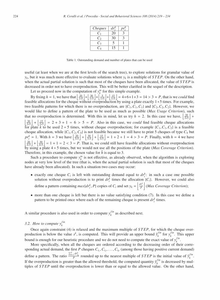
For instance, let us consider the following situation. We have 4 different cheques C1,C2,C3,C4 that

have to be placed on plates with P = 3 positions. The values of the outstanding demands and the number of

different plates where each cheque can still be placed are summarized in Table 1.

Assume we fix the value of S T EP equal to 5; this is the maximum common divisor of the outstanding

demands, and represents the minimum number of times a plate will be used. We point out that the use of this

parameter hugely decreases the number of possible solutions to be evaluated, without effecting too much the

quality of the final solution. Indeed, by analyzing the real case instances to be solved we observed that the

demand for each cheque was never less than 1000. Therefore, from a computational point of view it is not


Cheques drki prk

iC1 20 3

C2 30 3

C3 5 1

C4 15 1

Table 1. Outstanding demand and number of plates that can be used

useful (at least when we are at the first levels of the search tree), to explore solutions for granular value of

yk, but it was much more effective to evaluate solutions where yk is a multiple of S T EP. On the other hand,

when the actual partial solution is such that most of the cheques have been allocated, the value of S T EP is

decreased in order not to have overproduction. This will be better clarified in the sequel of the description.

Let us proceed now in the computation of yink for this simple example.

By fixing h = 1, we have that⌊

201∗5⌋+⌊

301∗5⌋+⌊

51∗5⌋+⌊

151∗5⌋= 4+6+1+3 = 14 > 3 = P, that is we could find

feasible allocations for the cheque without overproduction by using a plate exactly 1∗5 times. For example,

two feasible patterns for which there is no overproduction, are {C1,C1,C1} and {C2,C2,C2}. However, we

would like to define a pattern of the plate to be used as much as possible (Max Usage Criterion), such

that no overproduction is determined. With this in mind, let us try h = 2. In this case we have,⌊

202∗5⌋+⌊

302∗5⌋+⌊

152∗5⌋= 2 + 3 + 1 = 6 > 5 = P. Also in this case, we could find feasible cheque allocations

for plate k to be used 2 ∗ 5 times, without cheque overproduction; for example {C1,C1,C2} is a feasible

cheque allocation, while {C1,C2,C4} is not feasible because we still have to print 5 cheques of type C4 but

prki = 1. With h = 3 we have

⌊203∗5⌋+⌊

303∗5⌋+⌊

153∗5⌋= 1 + 2 + 1 = 4 > 3 = P. Finally, with h = 4 we have⌊

204∗5⌋+⌊

304∗5⌋= 1 + 1 = 2 < 3 = P. That is, we could still have feasible allocations without overproduction

by using a plate 4 ∗ 5 times, but we would not use all the positions of the plate (Max Coverage Criterion).

Therefore, in this example, the chosen value for h is equal to 3.

Such a procedure to compute yink is not effective, as already observed, when the algorithm is exploring

nodes at very low level of the tree (that is, when the actual partial solution is such that most of the cheques

have already been allocated). In such a situation two cases may occur:

• exactly one cheque Ci is left with outstanding demand equal to drki : in such a case one possible

solution without overproduction is to print drki times the allocation {Ci}. However, we could also

define a pattern containing max{drki , P} copies of Ci and set yk =

⌊drk

iP

⌋(Max Coverage Criterion);

• more than one cheque is left but there is no value satisfying condition (7). In this case we define a

pattern to be printed once where each of the remaining cheque is present drki times.

A similar procedure is also used in order to compute y f ink as described next.

3.2. How to compute y f ink

Once again constraint (4) is relaxed and the maximum multiple of S T EP, for which the cheque over-

production is below the value sk, is computed. This will provide an upper bound y f ink for y f in

k . This upper

bound is enough for our heuristic procedure and we do not need to compute the exact value of y f ink .

More specifically, when all the cheques are ordered according to the decreasing order of their corre-

sponding actual demand, the first P cheques Ci1 ,Ci2 , . . . ,CiP (among those having positive current demand)

define a pattern. The ratio

∑Ph=1 drk

ihP rounded up to the nearest multiple of S T EP is the initial value of y f in

k .

If the overproduction is greater than the allowed threshold, the computed quantity y f ink is decreased by mul-

tiples of S T EP until the overproduction is lower than or equal to the allowed value. On the other hand,


if the overproduction is lower than the allowed threshold y f ink is increased by multiples of S T EP until the

overproduction stays lower than or equal to the threshold.

Let us explain the procedure by an example.

Consider again 4 cheques as in Table 1. Assume sk = 10. We have P = 3 and S T EP = 5. We order

the cheques according to the decreasing order of their corresponding demand: {C2,C1,C4,C3}. We select

the first P cheques to define a pattern, compute the value

∑Ph=1 drk

ihP = 30+20+15

3= 21, round it up to the nearest

multiple of S T EP and fix y f ink to the obtained value, that is y f in

k = 25. The corresponding overproduction is

equal to 15 > sk, hence we set y f ink = 25 − S T EP = 20 that determines an allowed overproduction.

Before going into the details of the heuristic procedures, that are used to evaluate the feasible allocations

once the value yk has been fixed, let us make some observations.

3.3. Equivalent cheques and equivalent cheque allocationsConsider again the situation where we have to print 4 different cheques C1,C2,C3,C4 on plates with

3 positions. Suppose we are at level k, yk = 1 and the level of the demands are, respectively, drk1= 10,

drk2= 10, drk

3= 7, drk

4= 5. Then, we need to evaluate the costs of feasible allocations for plate k.

Consider the following two feasible allocations for plate k: {C1,C1,C3}, {C2,C2,C3}. They have the same

cost both in terms of used plate, and in terms of overproduced cheques. Two different nodes of the search

tree are associated with them, say Node 1 and Node 2, respectively. Note that, choosing either one of the

two allocations produces a “similar” typology of subtree to be explored. Indeed, with the former choice

we would have drk+11= 8, drk+1

2= 10, drk+1

3= 6, drk+1

4= 5, while with the latter one we would have

drk+11= 10, drk+1

2= 8, drk+1

3= 6, drk+1

4= 5.

The two subtrees rooted, respectively, at Node 1 and at Node 2 are similar in the sense that each node of

one subtree is “twin” of a node of the other. Indeed, each node in the first subtree has a companion node in

the second subtree associated with the same cheque allocation with cheque C1 replaced by cheque C2 (and

viceversa).

Therefore, it is evident that once we evaluate one of the two subtrees we do not need to evaluate the

other. We define the two allocations (corresponding to Node 1 and Node 2) to be “ equivalent” as formally

described next.

In these situations the algorithm evaluates the cheque allocation only once, and all the equivalent cheque

allocations are not considered. This simple observation allows us to substantially reduce the number of

“distinct” allocations to be considered.

From what above noticed it follows that we can reduce the search space by considering “equivalent”cheques and “equivalent” cheque allocations.

Definition 1: Two different cheques Ci and C j are said to be equivalent if the following two conditionshold: (i) di = d j and (ii) pi = p j.

We extend this definition to cheques Ci and C j such that drki = drk

j and prki = prk

j . That is, two differ-

ent cheques that were not equivalent at the beginning of the algorithm could become equivalent during the

execution of the algorithm. From Definition 1 the equivalence among cheque allocations follows directly.

Definition 2: Two feasible cheque allocations on the kth plate, are said to be equivalent if they only dif-fer in equivalent cheques.

Up to this point of the description we have shown how to compute yink and an upper bound on y f in

k . We

fix now yk in the interval [yink , y

f ink ] and consider various allocations of cheques. These procedures are de-

scribed in the next paragraph.

3.4. Fixing yk and evaluating different allocationsSuppose now, that the value of yk we consider is such that a cheque allocation with zero overproduction

exists (i.e. yk = yink ). In this case, distinct cheque allocations with zero overproduction are considered.


First, we sort the cheques for decreasing values of drki . Notice that, if a cheque is allocated on plate k that is

used yk times, there is no overproduction for that cheque if one of the following two conditions is satisfied:

drki ≡ 0 mod yk if prk

i = 1 (8)

drki ≥ yk if prk

i ≥ 2 (9)

Condition (8) is obvious: if cheque Ci cannot be present in additional plates (that is, prki = 1), we need

to satisfy the entire outstanding demand for it with one plate only. If such remaining demand is a multiple

of yk, that is drki ≡ 0 mod yk, there is no overproduction of cheque Ci. On the other hand (Condition (9)),

if we can use additional plates to produce cheque Ci (i.e., prki ≥ 2) and after using yk times plate k we still

have outstanding demand for that cheque, then the use of plate k does not produce extra cheques of type Ci.

All cheques, such that either (i) drki = yk and prk

i ≥ 2 or (ii) prki = 1 and drk

i ≡ 0 mod yk, are allocated

on plate k. Clearly, cheques in the second category will be allocated on the current plate k if and only if

there are enough free positions such that the cheque can be replicated the correct number of times. After

that, we fill the remaining free positions on the plate in all the possible (“distinct”) ways using cheques for

which drki > yk and prk

i ≥ 2. This cheques can be replicated between 0 and drki /yk times without cheque

overproduction.

When yk > yink , the algorithm does not find a feasible allocation of cheques on the plate k for which

cheque overproduction is zero. Among all the possible ways of allocating cheques with cheque overproduc-

tion below the current threshold sk, the one producing the minimum level of overproduction (among those

that are explored) is chosen.

In particular, the procedure tries to fill all the positions of the plate by choosing those cheques such that

drki ≥ yk and, then, fixing xik =

⌊drk

iyk

⌋. Successively, it fills the remaining positions by choosing one by one

the cheques according to the increasing order of their corresponding demands.

To better explain the proposed procedure, in the next paragraph we apply our algorithm to solve a simple

example with 4 types of cheques.

3.5. A complete example

We have to print 4 cheques C1,C2,C3,C4 on plates with P = 3 positions. The demand for each cheque

is, respectively, 10, 10, 7, 5. In order to make the example illustrative and not tedious we assume there is

not restriction on the number of different plates each cheque can be placed (i.e. pi = +∞, i = 1, 2, 3, 4).

The cost of an extra cheque is CC = 10, while the cost of an extra plate is CP = 20, therefore the allowable

cheque overproduction is S F = 2. Moreover, we set S T EP = 1. The corresponding search tree explored by

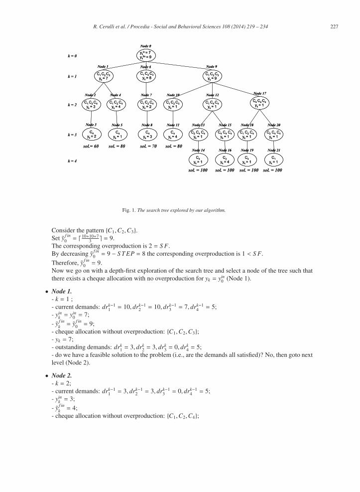
the algorithm is depicted in Figure 1.

• Node 0.At node 0 of the search tree we compute yin

0and y f in

0.

This range will determine the width of the entire search tree.

Let us determine yin0

. By fixing h = 1, we have:⌊

101∗1⌋+⌊

101∗1⌋+⌊

71∗1⌋+⌊

51∗1⌋= 10+ 10+ 7+ 5 = 32 >

3 = P;

- with h = 2, we have: 5 + 5 + 3 + 2 = 15 > 3;

- with h = 3, we have: 3 + 3 + 2 + 1 = 9 > 3;

- with h = 4, we have: 2 + 2 + 1 + 1 = 6 > 3;

- with h = 5, we have: 2 + 2 + 1 + 1 = 6 > 3;

- with h = 6, we have: 1 + 1 + 1 = 3;

- with h = 7, we have: 1 + 1 + 1 = 3;

- with h = 8, we have: 1 + 1 < 3.

Therefore, yin0= 7, for which a feasible pattern is {C1,C2,C3}.

Let us determine y f in0

.

Order the cheques according to the corresponding current demands.


Fig. 1. The search tree explored by our algorithm.

Consider the pattern {C1,C2,C3}.Set y f in

0= � 10+10+7

3 = 9.

The corresponding overproduction is 2 = S F.

By decreasing y f in0= 9 − S T EP = 8 the corresponding overproduction is 1 < S F.

Therefore, y f in0= 9.

Now we go on with a depth-first exploration of the search tree and select a node of the tree such that

there exists a cheque allocation with no overproduction for yk = yin0

(Node 1).

• Node 1.- k = 1 ;

- current demands: drk−11= 10, drk−1

2= 10, drk−1

3= 7, drk−1

4= 5;

- yink = yin

0= 7;

- y f ink = y f in

0= 9;

- cheque allocation without overproduction: {C1,C2,C3};- yk = 7;

- outstanding demands: drk1= 3, drk

2= 3, drk

3= 0, drk

4= 5;

- do we have a feasible solution to the problem (i.e., are the demands all satisfied)? No, then goto next

level (Node 2).

• Node 2.- k = 2;


2= 3, drk−1

3= 0, drk−1

4= 5;

- yink = 3;

- y f ink = 4;

- cheque allocation without overproduction: {C1,C2,C4};


- yk = 3;


2= 0, drk

3= 0, drk

4= 2;

- Is this a feasible solution? No, then goto next level (Node 3).

• Node 3.- k = 3;


2= 0, drk−1

3= 0, drk−1

4= 2;

- yink = 2;

- cheque allocation without overproduction: {C4};- yk = 2;


2= 0, drk

3= 0, drk

4= 0;

- Is this a feasible solution? Yes, value of the solution: 60;

- backtrack (Node 4).

• Node 4.- k = 2;


2= 3, drk−1

3= 0, drk−1

4= 5;

- yink = 3;

- y f ink = 4;

- cheque allocation without overproduction (different from Node 2): it does not exist;

- cheque allocation with allowed overproduction: {C1,C2,C4} and yk = 4;

- overproduction is equal to 2: sk = 0;


2= 0, drk

3= 0, drk

4= 1;

- Is this a feasible solution? No, then go to next level (Node 5).

• Node 5.- k = 3;


2= 0, drk−1

3= 0, drk−1

4= 1;

- yink = 1;

- cheque allocation without overproduction: {C4};- yk = 1;


2= 0, drk

3= 0, drk

4= 0;

- Is this a feasible solution? Yes, value of the solution: 60 + 20 = 80;


• Node 6.- k = 1;


2= 10, drk−1

3= 7, drk−1

4= 5;

- yink = 7;

- y f ink = 9;


- cheque allocation with allowed overproduction: {C1,C2,C3} and yk = 8;



2= 2, drk

3= 0, drk

4= 5;


• Node 7.- k = 2;


2= 2, drk−1

3= 0, drk−1

4= 5;

- yink = 2;

- y f ink = 2;

- cheque allocation without overproduction: {C1,C2,C4};



2= 0, drk

3= 0, drk

4= 3;


• Node 8.- k = 3;


2= 0, drk−1

3= 0, drk−1

4= 3;

- yink = 3;

- cheque allocation without overproduction : {C4};- yk = 3;


2= 0, drk

3= 0, drk

4= 0;



• Node 9.- k = 1;


2= 10, drk−1

3= 7, drk−1

4= 5;

- yink = 7;

- y f ink = 9;


- cheque allocation with allowed overproduction (different from Node 6) : {C1,C2,C3} and yk = 9;



2= 1, drk

3= 0, drk

4= 5;


• Node 10.- k = 2;


2= 1, drk−1

3= 0, drk−1

4= 5;

- yink = 1;

- y f ink = 1;

- cheque allocation without overproduction: {C1,C2,C4};- outstanding demands: drk

1= 0, drk

2= 0, drk

3= 0, drk

4= 4;


• Node 11.- k = 3;


2= 0, drk−1

3= 0, drk−1

4= 4;

- yink = 4;

- y f ink = 4;

- cheque allocation without overproduction : {C4};- yk = 4;


2= 0, drk

3= 0, drk

4= 0;



The algorithm continues in this way, until all the possible nodes of the tree have been explored. It stops

returning the best solution determined so far, that, for this simple example, is also optimal and corresponds

to the path in the tree: Node 1 - Node 2 - Node 3.

We want to point out again that the width of the search tree that is explored mainly depends on: (i) the

ranges [yink , y

f ink ], (ii) the granularity of the value fixed for yk (that is the value of S T EP), (iii) the feasible

“distinct” allocations explored once yk is fixed. In particular, for this example note that once Node 20 is

explored with cheque allocation {C2,C4,C4} then the equivalent allocation {C1,C4,C4} is not considered at

all.


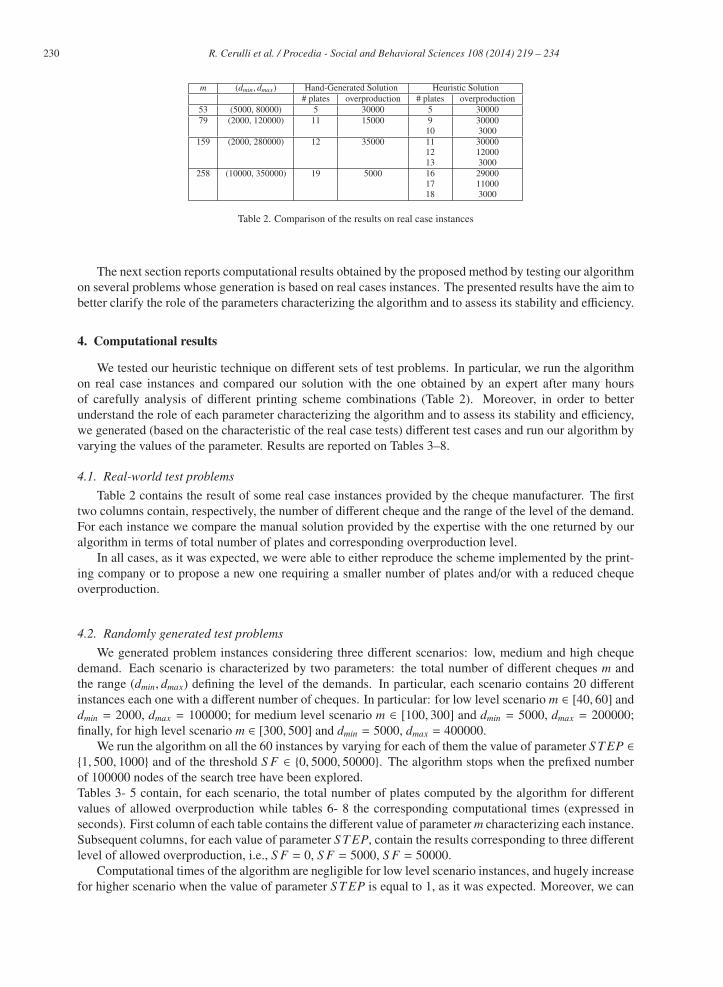
m (dmin, dmax) Hand-Generated Solution Heuristic Solution

# plates overproduction # plates overproduction

53 (5000, 80000) 5 30000 5 30000

79 (2000, 120000) 11 15000 9 3000010 3000

159 (2000, 280000) 12 35000 11 3000012 1200013 3000

258 (10000, 350000) 19 5000 16 2900017 1100018 3000

Table 2. Comparison of the results on real case instances

The next section reports computational results obtained by the proposed method by testing our algorithm

on several problems whose generation is based on real cases instances. The presented results have the aim to

better clarify the role of the parameters characterizing the algorithm and to assess its stability and efficiency.

4. Computational results

We tested our heuristic technique on different sets of test problems. In particular, we run the algorithm

on real case instances and compared our solution with the one obtained by an expert after many hours

of carefully analysis of different printing scheme combinations (Table 2). Moreover, in order to better

understand the role of each parameter characterizing the algorithm and to assess its stability and efficiency,

we generated (based on the characteristic of the real case tests) different test cases and run our algorithm by

varying the values of the parameter. Results are reported on Tables 3–8.

4.1. Real-world test problemsTable 2 contains the result of some real case instances provided by the cheque manufacturer. The first

two columns contain, respectively, the number of different cheque and the range of the level of the demand.

For each instance we compare the manual solution provided by the expertise with the one returned by our

algorithm in terms of total number of plates and corresponding overproduction level.

In all cases, as it was expected, we were able to either reproduce the scheme implemented by the print-

ing company or to propose a new one requiring a smaller number of plates and/or with a reduced cheque

overproduction.

4.2. Randomly generated test problemsWe generated problem instances considering three different scenarios: low, medium and high cheque

demand. Each scenario is characterized by two parameters: the total number of different cheques m and

the range (dmin, dmax) defining the level of the demands. In particular, each scenario contains 20 different

instances each one with a different number of cheques. In particular: for low level scenario m ∈ [40, 60] and

dmin = 2000, dmax = 100000; for medium level scenario m ∈ [100, 300] and dmin = 5000, dmax = 200000;

finally, for high level scenario m ∈ [300, 500] and dmin = 5000, dmax = 400000.

We run the algorithm on all the 60 instances by varying for each of them the value of parameter S T EP ∈{1, 500, 1000} and of the threshold S F ∈ {0, 5000, 50000}. The algorithm stops when the prefixed number

of 100000 nodes of the search tree have been explored.

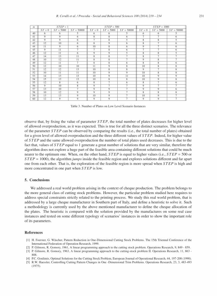
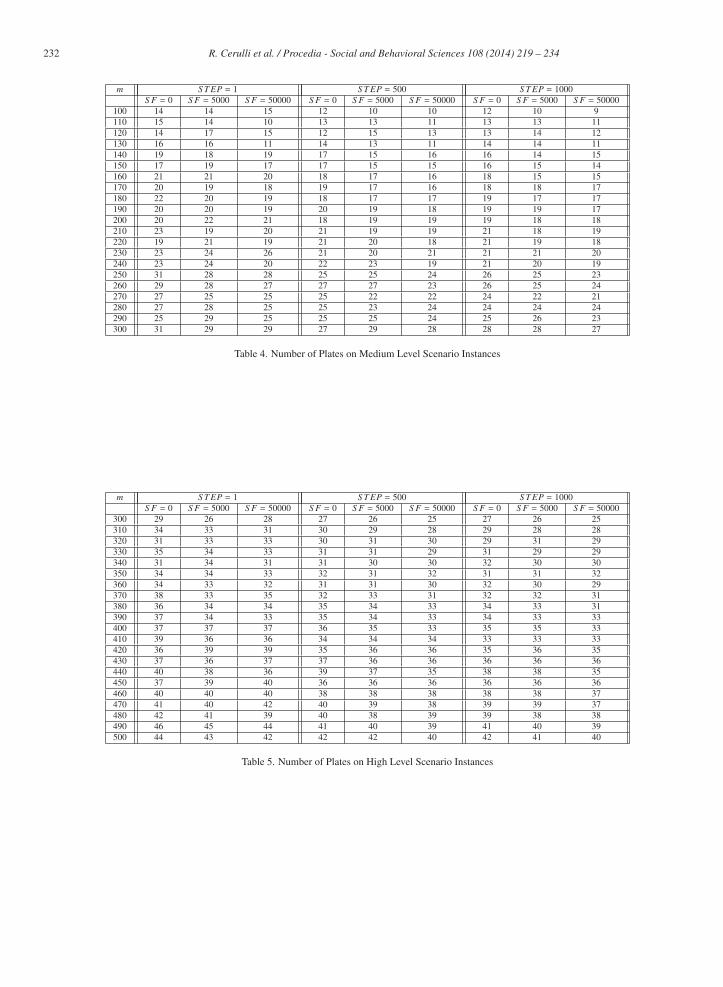
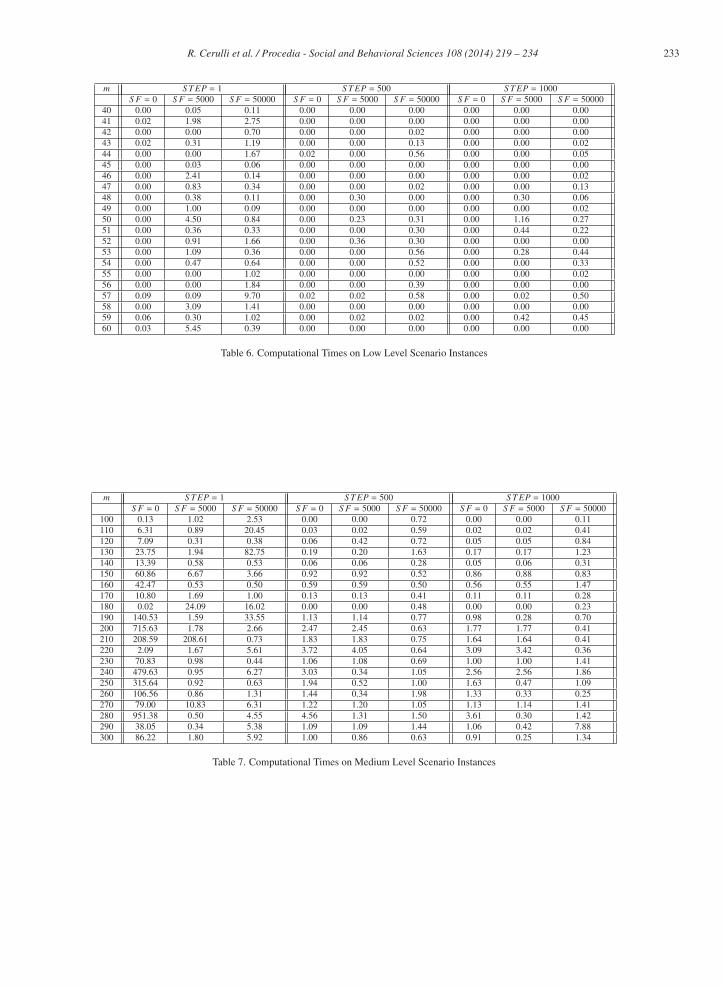
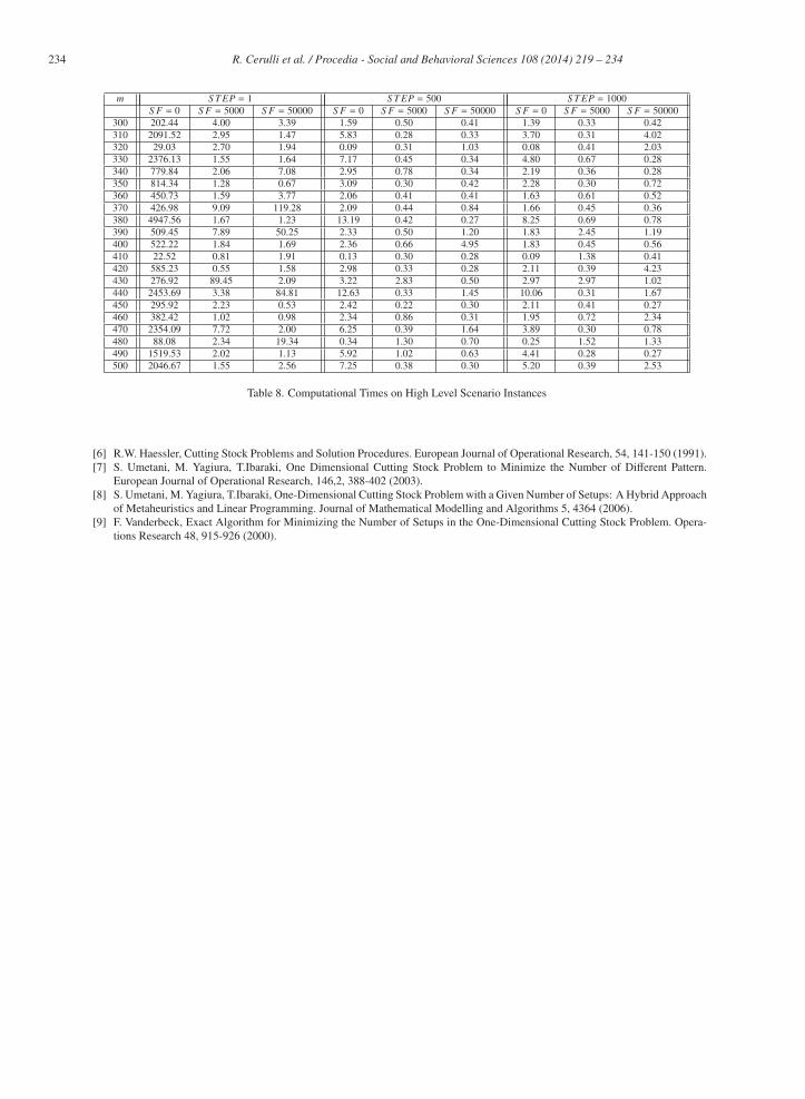
Tables 3- 5 contain, for each scenario, the total number of plates computed by the algorithm for different

values of allowed overproduction while tables 6- 8 the corresponding computational times (expressed in

seconds). First column of each table contains the different value of parameter m characterizing each instance.

Subsequent columns, for each value of parameter S T EP, contain the results corresponding to three different

level of allowed overproduction, i.e., S F = 0, S F = 5000, S F = 50000.

Computational times of the algorithm are negligible for low level scenario instances, and hugely increase

for higher scenario when the value of parameter S T EP is equal to 1, as it was expected. Moreover, we can


m S T EP = 1 S T EP = 500 S T EP = 1000

S F = 0 S F = 5000 S F = 50000 S F = 0 S F = 5000 S F = 50000 S F = 0 S F = 5000 S F = 50000

40 6 6 5 6 6 5 6 6 5

41 9 9 6 8 8 6 7 7 6

42 9 9 6 7 8 5 8 8 5

43 12 10 6 8 9 6 8 7 6

44 11 9 6 10 8 6 9 7 6

45 9 11 7 7 8 6 7 7 6

46 12 11 6 9 9 5 8 8 5

47 14 13 11 8 8 7 8 7 7

48 10 12 11 8 8 7 9 8 7

49 12 11 7 8 8 6 8 8 6

50 12 10 10 11 9 8 10 8 8

51 12 12 13 10 8 8 9 7 8

52 10 11 11 10 9 9 10 8 8

53 14 13 13 10 9 11 10 9 9

54 15 13 13 10 8 8 10 9 8

55 12 8 6 8 7 6 8 7 6

56 9 10 8 9 7 7 9 7 7

57 13 10 7 9 9 7 9 9 6

58 10 12 9 9 9 7 8 8 8

59 13 13 9 10 9 7 10 9 7

60 12 9 9 9 9 7 9 9 7

Table 3. Number of Plates on Low Level Scenario Instances

observe that, by fixing the value of parameter S T EP, the total number of plates decreases for higher level

of allowed overproduction, as it was expected. This is true for all the three distinct scenarios. The relevance

of the parameter S T EP can be observed by comparing the results (i.e., the total number of plates) obtained

for a given level of allowed overproduction and the three different values of S T EP. Indeed, for higher value

of S T EP and the same allowed overproduction the number of total plates used decreases. This is due to the

fact that, values of S T EP equal to 1 generate a great number of solutions that are very similar, therefore the

algorithm does not explore a huge part of the feasible area containing different solutions that could be much

nearer to the optimum one. When, on the other hand, S T EP is equal to higher values (i.e., S T EP = 500 or

S T EP = 1000), the algorithm jumps inside the feasible region and explores solutions different and far apart

one from each other. That is, the exploration of the feasible region is more spread when S T EP is high and

more concentrated in one part when S T EP is low.

5. Conclusions

We addressed a real world problem arising in the context of cheque production. The problem belongs to

the more general class of cutting stock problems. However, the particular problem studied here requires to

address special constraints strictly related to the printing process. We study this real world problem, that is

addressed by a large cheque manufacturer in Southern part of Italy, and define a heuristic to solve it. Such

a methodology is currently used by the above mentioned manufacturer to define the cheque allocation of

the plates. The heuristic is compared with the solution provided by the manufactures on some real case

instances and tested on some different typology of scenarios’ instances in order to show the important role

of its parameters.

References

[1] H. Foerster, G. Wascher, Pattern Reduction in One-Dimensional Cutting Stock Problems. The 15th Triennal Conference of the

International Federation of Operation Research, 1999.

[2] P. Gilmore, R. Gomory, 1961, A linear programming approach to the cutting stock problem. Operations Research, 9, 849 - 859.

[3] P. Gilmore, R. Gomory, 1963, A linear programming approach to the cutting-stock problem II. Operations Research, 11, 863 -

888.

[4] P.C. Goulimis, Optimal Solutions for the Cutting Stock Problem, European Journal of Operational Research, 44, 197-208 (1990).

[5] R.W. Haessler, Controlling Cutting Pattern Changes in One -Dimensional Trim Problems. Operations Research, 23, 3, 483-493

(1975).


m S T EP = 1 S T EP = 500 S T EP = 1000


100 14 14 15 12 10 10 12 10 9

110 15 14 10 13 13 11 13 13 11

120 14 17 15 12 15 13 13 14 12

130 16 16 11 14 13 11 14 14 11

140 19 18 19 17 15 16 16 14 15

150 17 19 17 17 15 15 16 15 14

160 21 21 20 18 17 16 18 15 15

170 20 19 18 19 17 16 18 18 17

180 22 20 19 18 17 17 19 17 17

190 20 20 19 20 19 18 19 19 17

200 20 22 21 18 19 19 19 18 18

210 23 19 20 21 19 19 21 18 19

220 19 21 19 21 20 18 21 19 18

230 23 24 26 21 20 21 21 21 20

240 23 24 20 22 23 19 21 20 19

250 31 28 28 25 25 24 26 25 23

260 29 28 27 27 27 23 26 25 24

270 27 25 25 25 22 22 24 22 21

280 27 28 25 25 23 24 24 24 24

290 25 29 25 25 25 24 25 26 23

300 31 29 29 27 29 28 28 28 27

Table 4. Number of Plates on Medium Level Scenario Instances

m S T EP = 1 S T EP = 500 S T EP = 1000


300 29 26 28 27 26 25 27 26 25

310 34 33 31 30 29 28 29 28 28

320 31 33 33 30 31 30 29 31 29

330 35 34 33 31 31 29 31 29 29

340 31 34 31 31 30 30 32 30 30

350 34 34 33 32 31 32 31 31 32

360 34 33 32 31 31 30 32 30 29

370 38 33 35 32 33 31 32 32 31

380 36 34 34 35 34 33 34 33 31

390 37 34 33 35 34 33 34 33 33

400 37 37 37 36 35 33 35 35 33

410 39 36 36 34 34 34 33 33 33

420 36 39 39 35 36 36 35 36 35

430 37 36 37 37 36 36 36 36 36

440 40 38 36 39 37 35 38 38 35

450 37 39 40 36 36 36 36 36 36

460 40 40 40 38 38 38 38 38 37

470 41 40 42 40 39 38 39 39 37

480 42 41 39 40 38 39 39 38 38

490 46 45 44 41 40 39 41 40 39

500 44 43 42 42 42 40 42 41 40

Table 5. Number of Plates on High Level Scenario Instances


m S T EP = 1 S T EP = 500 S T EP = 1000


40 0.00 0.05 0.11 0.00 0.00 0.00 0.00 0.00 0.00

41 0.02 1.98 2.75 0.00 0.00 0.00 0.00 0.00 0.00

42 0.00 0.00 0.70 0.00 0.00 0.02 0.00 0.00 0.00

43 0.02 0.31 1.19 0.00 0.00 0.13 0.00 0.00 0.02

44 0.00 0.00 1.67 0.02 0.00 0.56 0.00 0.00 0.05

45 0.00 0.03 0.06 0.00 0.00 0.00 0.00 0.00 0.00

46 0.00 2.41 0.14 0.00 0.00 0.00 0.00 0.00 0.02

47 0.00 0.83 0.34 0.00 0.00 0.02 0.00 0.00 0.13

48 0.00 0.38 0.11 0.00 0.30 0.00 0.00 0.30 0.06

49 0.00 1.00 0.09 0.00 0.00 0.00 0.00 0.00 0.02

50 0.00 4.50 0.84 0.00 0.23 0.31 0.00 1.16 0.27

51 0.00 0.36 0.33 0.00 0.00 0.30 0.00 0.44 0.22

52 0.00 0.91 1.66 0.00 0.36 0.30 0.00 0.00 0.00

53 0.00 1.09 0.36 0.00 0.00 0.56 0.00 0.28 0.44

54 0.00 0.47 0.64 0.00 0.00 0.52 0.00 0.00 0.33

55 0.00 0.00 1.02 0.00 0.00 0.00 0.00 0.00 0.02

56 0.00 0.00 1.84 0.00 0.00 0.39 0.00 0.00 0.00

57 0.09 0.09 9.70 0.02 0.02 0.58 0.00 0.02 0.50

58 0.00 3.09 1.41 0.00 0.00 0.00 0.00 0.00 0.00

59 0.06 0.30 1.02 0.00 0.02 0.02 0.00 0.42 0.45

60 0.03 5.45 0.39 0.00 0.00 0.00 0.00 0.00 0.00

Table 6. Computational Times on Low Level Scenario Instances

m S T EP = 1 S T EP = 500 S T EP = 1000


100 0.13 1.02 2.53 0.00 0.00 0.72 0.00 0.00 0.11

110 6.31 0.89 20.45 0.03 0.02 0.59 0.02 0.02 0.41

120 7.09 0.31 0.38 0.06 0.42 0.72 0.05 0.05 0.84

130 23.75 1.94 82.75 0.19 0.20 1.63 0.17 0.17 1.23

140 13.39 0.58 0.53 0.06 0.06 0.28 0.05 0.06 0.31

150 60.86 6.67 3.66 0.92 0.92 0.52 0.86 0.88 0.83

160 42.47 0.53 0.50 0.59 0.59 0.50 0.56 0.55 1.47

170 10.80 1.69 1.00 0.13 0.13 0.41 0.11 0.11 0.28

180 0.02 24.09 16.02 0.00 0.00 0.48 0.00 0.00 0.23

190 140.53 1.59 33.55 1.13 1.14 0.77 0.98 0.28 0.70

200 715.63 1.78 2.66 2.47 2.45 0.63 1.77 1.77 0.41

210 208.59 208.61 0.73 1.83 1.83 0.75 1.64 1.64 0.41

220 2.09 1.67 5.61 3.72 4.05 0.64 3.09 3.42 0.36

230 70.83 0.98 0.44 1.06 1.08 0.69 1.00 1.00 1.41

240 479.63 0.95 6.27 3.03 0.34 1.05 2.56 2.56 1.86

250 315.64 0.92 0.63 1.94 0.52 1.00 1.63 0.47 1.09

260 106.56 0.86 1.31 1.44 0.34 1.98 1.33 0.33 0.25

270 79.00 10.83 6.31 1.22 1.20 1.05 1.13 1.14 1.41

280 951.38 0.50 4.55 4.56 1.31 1.50 3.61 0.30 1.42

290 38.05 0.34 5.38 1.09 1.09 1.44 1.06 0.42 7.88

300 86.22 1.80 5.92 1.00 0.86 0.63 0.91 0.25 1.34

Table 7. Computational Times on Medium Level Scenario Instances


m S T EP = 1 S T EP = 500 S T EP = 1000


300 202.44 4.00 3.39 1.59 0.50 0.41 1.39 0.33 0.42

310 2091.52 2.95 1.47 5.83 0.28 0.33 3.70 0.31 4.02

320 29.03 2.70 1.94 0.09 0.31 1.03 0.08 0.41 2.03

330 2376.13 1.55 1.64 7.17 0.45 0.34 4.80 0.67 0.28

340 779.84 2.06 7.08 2.95 0.78 0.34 2.19 0.36 0.28

350 814.34 1.28 0.67 3.09 0.30 0.42 2.28 0.30 0.72

360 450.73 1.59 3.77 2.06 0.41 0.41 1.63 0.61 0.52

370 426.98 9.09 119.28 2.09 0.44 0.84 1.66 0.45 0.36

380 4947.56 1.67 1.23 13.19 0.42 0.27 8.25 0.69 0.78

390 509.45 7.89 50.25 2.33 0.50 1.20 1.83 2.45 1.19

400 522.22 1.84 1.69 2.36 0.66 4.95 1.83 0.45 0.56

410 22.52 0.81 1.91 0.13 0.30 0.28 0.09 1.38 0.41

420 585.23 0.55 1.58 2.98 0.33 0.28 2.11 0.39 4.23

430 276.92 89.45 2.09 3.22 2.83 0.50 2.97 2.97 1.02

440 2453.69 3.38 84.81 12.63 0.33 1.45 10.06 0.31 1.67

450 295.92 2.23 0.53 2.42 0.22 0.30 2.11 0.41 0.27

460 382.42 1.02 0.98 2.34 0.86 0.31 1.95 0.72 2.34

470 2354.09 7.72 2.00 6.25 0.39 1.64 3.89 0.30 0.78

480 88.08 2.34 19.34 0.34 1.30 0.70 0.25 1.52 1.33

490 1519.53 2.02 1.13 5.92 1.02 0.63 4.41 0.28 0.27

500 2046.67 1.55 2.56 7.25 0.38 0.30 5.20 0.39 2.53

Table 8. Computational Times on High Level Scenario Instances

[6] R.W. Haessler, Cutting Stock Problems and Solution Procedures. European Journal of Operational Research, 54, 141-150 (1991).

[7] S. Umetani, M. Yagiura, T.Ibaraki, One Dimensional Cutting Stock Problem to Minimize the Number of Different Pattern.

European Journal of Operational Research, 146,2, 388-402 (2003).

[8] S. Umetani, M. Yagiura, T.Ibaraki, One-Dimensional Cutting Stock Problem with a Given Number of Setups: A Hybrid Approach

of Metaheuristics and Linear Programming. Journal of Mathematical Modelling and Algorithms 5, 4364 (2006).

[9] F. Vanderbeck, Exact Algorithm for Minimizing the Number of Setups in the One-Dimensional Cutting Stock Problem. Opera-

tions Research 48, 915-926 (2000).