Gravity Equations:
Workhorse,Toolkit, and Cookbook∗
Keith Head† Thierry Mayer‡
April 7, 2013
Abstract
This chapter focuses on the estimation and interpretation of gravity equations for bilateral
trade. This necessarily involves a careful consideration of the theoretical underpinnings since
it has become clear that naive approaches to estimation lead to biased and frequently misin-
terpreted results. There are now several theory-consistent estimation methods and we argue
against sole reliance on any one method and instead advocate a toolkit approach. One estima-
tor may be preferred for certain types of data or research questions but more often the methods
should be used in concert to establish robustness. In recent years, estimation has become just
a first step before a deeper analysis of the implications of the results, notably in terms of wel-
fare. We try to facilitate diffusion of best-practice methods by illustrating their application in
a step-by-step cookbook mode of exposition.
JEL code: F1
Keywords: bilateral trade, heterogeneous firms, distance, borders, trade cost elasticity, poisson
∗The chapter has a companion website, https://sites.google.com/site/hiegravity/, with an appendix, Statacode, and related links. We thank Leo Fankhanel and Camilo Umana for outstanding assistance with the programmingand meta-analysis in this chapter, Soledad Zignago for great help with providing and understanding subtleties ofsome of the data used, and Julia Jauer for her update of the gravity data. Scott Baier, Sebastian Sotelo, Joao SantosSilva generously provided computer code. Andres Rodrıguez-Clare answered many questions we had about welfarecalculations but is not responsible of course, for any mistakes we may have made. Arnaud Costinot, Gilles Duranton,Thibault Fally, Mario Larch, Marc Melitz, Gianmarco Ottaviano, Joao Santos Silva, and Daniel Trefler made veryuseful comments on previous drafts. We are especially grateful to Jose de Sousa: his careful reading identified manynecessary corrections in an early draft. Participants at presentations Hitotsubashi GCOE Conference on InternationalTrade and FDI 2012, National Bank of Belgium, Clemson University also contributed to improving the draft. Finally,we thank our discussants at the handbook conference, Rob Feenstra and Jim Anderson, for many helpful suggestions.We regret that because of limitations of time and space, we have not been able to fully respond to all of the valuablesuggestions we received. This research has received funding from the European Research Council under the EuropeanCommunity’s Seventh Framework Programme (FP7/2007-2013) Grant Agreement no. 313522.†Sauder School of Business, University of British Columbia and CEPR, [email protected]‡Sciences Po, CEPII, and CEPR, [email protected]
1
Contents
1 Introduction 3
1.1 Gravity features of trade data . . . . . . . . . . . . . . . . . . . . . . . . . . . . . . . 3
1.2 A brief history of gravity in trade . . . . . . . . . . . . . . . . . . . . . . . . . . . . . 5
2 Microfoundations for Gravity Equations 7
2.1 Three Definitions of the Gravity Equation . . . . . . . . . . . . . . . . . . . . . . . . 8
2.2 Assumptions underlying structural gravity . . . . . . . . . . . . . . . . . . . . . . . . 10
2.3 Main variants of gravity for trade . . . . . . . . . . . . . . . . . . . . . . . . . . . . . 11
2.4 Gravity models beyond trade in goods . . . . . . . . . . . . . . . . . . . . . . . . . . 19
3 Theory-consistent estimation 19
3.1 Proxies for multilateral resistance terms . . . . . . . . . . . . . . . . . . . . . . . . . 20
3.2 Iterative structural estimation . . . . . . . . . . . . . . . . . . . . . . . . . . . . . . . 20
3.3 Fixed effects estimation . . . . . . . . . . . . . . . . . . . . . . . . . . . . . . . . . . 21
3.4 Ratio-type estimation . . . . . . . . . . . . . . . . . . . . . . . . . . . . . . . . . . . 22
3.5 Other methods . . . . . . . . . . . . . . . . . . . . . . . . . . . . . . . . . . . . . . . 23
3.6 Monte Carlo study of alternative estimators . . . . . . . . . . . . . . . . . . . . . . . 23
3.7 Identification and estimation of country-specific effects . . . . . . . . . . . . . . . . . 27
4 Gravity estimates of policy impacts 29
4.1 Meta-analysis of policy dummies . . . . . . . . . . . . . . . . . . . . . . . . . . . . . 29
4.2 The elasticity of trade with respect to trade costs . . . . . . . . . . . . . . . . . . . . 32
4.3 Partial vs general equilibrium impacts on trade . . . . . . . . . . . . . . . . . . . . . 34
4.4 Testing structural gravity . . . . . . . . . . . . . . . . . . . . . . . . . . . . . . . . . 39
5 Frontiers of gravity research 41
5.1 Gravity’s errors . . . . . . . . . . . . . . . . . . . . . . . . . . . . . . . . . . . . . . . 41
5.2 Causes and consequences of zeros . . . . . . . . . . . . . . . . . . . . . . . . . . . . . 45
5.3 Firm-level gravity, extensive and intensive margins . . . . . . . . . . . . . . . . . . . 51
6 Directions for future research 57
7 Conclusions 57
References 57
2
1 Introduction
As the name suggests, gravity equations are a model of bilateral interactions in which size and
distance effects enter multiplicatively. They have been used as a workhorse for analyzing the
determinants of bilateral trade flows for 50 years since being introduced by Tinbergen (1962).
Krugman (1997) referred to gravity equations as examples of “social physics,” the relatively few law-
like empirical regularities that characterize social interactions.1 Over the last decade, concentrated
efforts of trade theorists have established that gravity equations emerge from mainstream modeling
frameworks in economics and should no longer be thought of as deriving from some murky analogy
with Newtonian physics. Meanwhile empirical work—guided in varying degrees by the new theory—
has proceeded to lay down a raft of stylized facts about the determinants of bilateral trade. As a
result of recent modelling, we now know that gravity estimates can be combined with trade policy
experiments to calculate implied welfare changes.
This chapter focuses on the estimation and interpretation of gravity equations for bilateral
trade. This necessarily involves a careful consideration of the theoretical underpinnings since it
has become clear that naive approaches to estimation lead to biased and frequently misinterpreted
results. There are now several theory-consistent estimation methods and we argue against sole
reliance on any one method and instead advocate a toolkit approach. One estimator may be
preferred for certain types of data or research questions but more often the methods should be used
in concert to establish robustness. In recent years, estimation has become just a first step before a
deeper analysis of the implications of the results, notably in terms of welfare. We try to facilitate
diffusion of best-practice methods by illustrating their application in a step-by-step cookbook mode
of exposition.
1.1 Gravity features of trade data
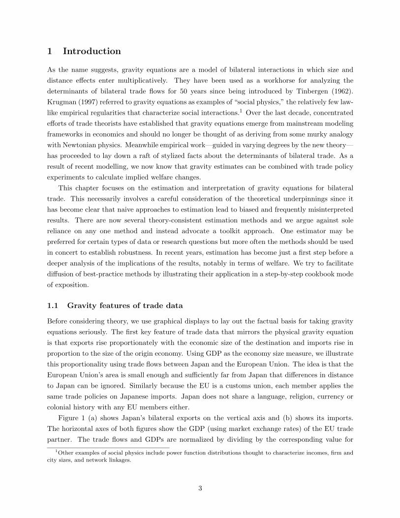
Before considering theory, we use graphical displays to lay out the factual basis for taking gravity
equations seriously. The first key feature of trade data that mirrors the physical gravity equation
is that exports rise proportionately with the economic size of the destination and imports rise in
proportion to the size of the origin economy. Using GDP as the economy size measure, we illustrate
this proportionality using trade flows between Japan and the European Union. The idea is that the
European Union’s area is small enough and sufficiently far from Japan that differences in distance
to Japan can be ignored. Similarly because the EU is a customs union, each member applies the
same trade policies on Japanese imports. Japan does not share a language, religion, currency or
colonial history with any EU members either.
Figure 1 (a) shows Japan’s bilateral exports on the vertical axis and (b) shows its imports.
The horizontal axes of both figures show the GDP (using market exchange rates) of the EU trade
partner. The trade flows and GDPs are normalized by dividing by the corresponding value for
1Other examples of social physics include power function distributions thought to characterize incomes, firm andcity sizes, and network linkages.
3
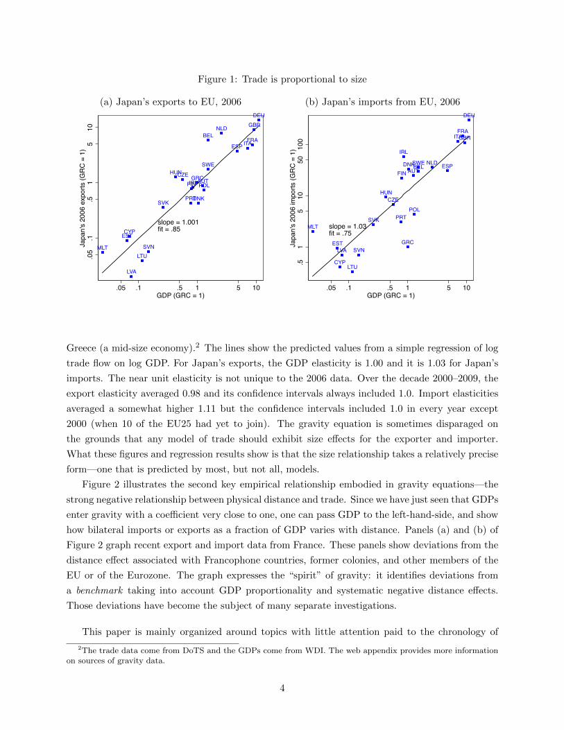
Figure 1: Trade is proportional to size
(a) Japan’s exports to EU, 2006 (b) Japan’s imports from EU, 2006
MLT
ESTCYP
LVA
LTUSVN
SVK
HUNCZE
PRT
FINIRLGRC
DNK
AUTPOL
SWE
BELNLD
ESP ITAFRA
GBRDEU
slope = 1.001fit = .85
.05
.1.5
15
10Ja
pan'
s 20
06 e
xpor
ts (G
RC =
1)
.05 .1 .5 1 5 10GDP (GRC = 1)
MLT
EST
CYP
LVA
LTU
SVN
SVK
HUNCZE
PRT
FIN
IRL
GRC
DNKAUT
POL
SWEBELNLD ESP
ITAFRAGBR
DEU
slope = 1.03fit = .75
.51
510
5010
0Ja
pan'
s 20
06 im
ports
(GRC
= 1
).05 .1 .5 1 5 10
GDP (GRC = 1)
Greece (a mid-size economy).2 The lines show the predicted values from a simple regression of log
trade flow on log GDP. For Japan’s exports, the GDP elasticity is 1.00 and it is 1.03 for Japan’s
imports. The near unit elasticity is not unique to the 2006 data. Over the decade 2000–2009, the
export elasticity averaged 0.98 and its confidence intervals always included 1.0. Import elasticities
averaged a somewhat higher 1.11 but the confidence intervals included 1.0 in every year except
2000 (when 10 of the EU25 had yet to join). The gravity equation is sometimes disparaged on
the grounds that any model of trade should exhibit size effects for the exporter and importer.
What these figures and regression results show is that the size relationship takes a relatively precise
form—one that is predicted by most, but not all, models.
Figure 2 illustrates the second key empirical relationship embodied in gravity equations—the
strong negative relationship between physical distance and trade. Since we have just seen that GDPs
enter gravity with a coefficient very close to one, one can pass GDP to the left-hand-side, and show
how bilateral imports or exports as a fraction of GDP varies with distance. Panels (a) and (b) of
Figure 2 graph recent export and import data from France. These panels show deviations from the
distance effect associated with Francophone countries, former colonies, and other members of the
EU or of the Eurozone. The graph expresses the “spirit” of gravity: it identifies deviations from
a benchmark taking into account GDP proportionality and systematic negative distance effects.
Those deviations have become the subject of many separate investigations.
This paper is mainly organized around topics with little attention paid to the chronology of
2The trade data come from DoTS and the GDPs come from WDI. The web appendix provides more informationon sources of gravity data.
4
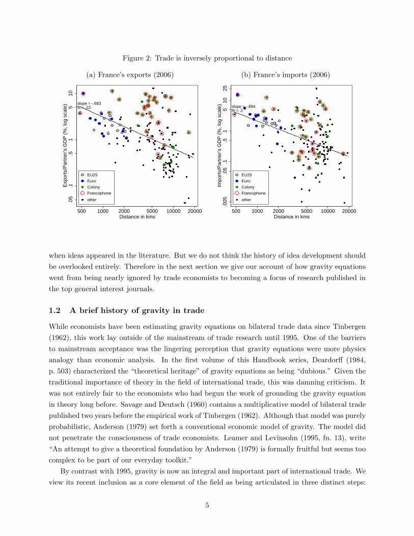
Figure 2: Trade is inversely proportional to distance
(a) France’s exports (2006) (b) France’s imports (2006)
slope = -.683fit = .22
.005
.05
.1.5
15
10E
xpor
ts/P
artn
er's
GD
P (
%, l
og s
cale
)
500 1000 2000 5000 10000 20000Distance in kms
EU25
Euro
Colony
Francophone
other
slope = -.894fit = .2
.005
.05
.1.5
15
1025
Impo
rts/
Par
tner
's G
DP
(%
, log
sca
le)
500 1000 2000 5000 10000 20000Distance in kms
EU25
Euro
Colony
Francophone
other
when ideas appeared in the literature. But we do not think the history of idea development should
be overlooked entirely. Therefore in the next section we give our account of how gravity equations
went from being nearly ignored by trade economists to becoming a focus of research published in
the top general interest journals.
1.2 A brief history of gravity in trade
While economists have been estimating gravity equations on bilateral trade data since Tinbergen
(1962), this work lay outside of the mainstream of trade research until 1995. One of the barriers
to mainstream acceptance was the lingering perception that gravity equations were more physics
analogy than economic analysis. In the first volume of this Handbook series, Deardorff (1984,
p. 503) characterized the “theoretical heritage” of gravity equations as being “dubious.” Given the
traditional importance of theory in the field of international trade, this was damning criticism. It
was not entirely fair to the economists who had begun the work of grounding the gravity equation
in theory long before. Savage and Deutsch (1960) contains a multiplicative model of bilateral trade
published two years before the empirical work of Tinbergen (1962). Although that model was purely
probabilistic, Anderson (1979) set forth a conventional economic model of gravity. The model did
not penetrate the consciousness of trade economists. Leamer and Levinsohn (1995, fn. 13), write
“An attempt to give a theoretical foundation by Anderson (1979) is formally fruitful but seems too
complex to be part of our everyday toolkit.”
By contrast with 1995, gravity is now an integral and important part of international trade. We
view its recent inclusion as a core element of the field as being articulated in three distinct steps:
5
the “admission” wherein researchers realized there was a surprisingly large amount of missing trade,
and admitted that gravity was one way to measure and explain it. Then came the “multilateral re-
sistance/fixed effects revolution,” a burst of papers that established the relationship between fixed
effects in gravity and underlying theories with origins as varied as Ricardo, monopolistic compe-
tition, and Armington. The final step was one of “convergence” of the gravity and heterogenous
firms literatures.
Admission (1995): 1995 was a very important year for gravity research. In that year Trefler
(1995) introduced the idea of “missing trade.” A key empirical problem for the HOV model is
that it predicts much higher trade in factor services than is actually observed. Trefler invoked
“home bias” rather than distance to explain missing trade but his work pointed to the importance
of understanding the impediments to trade. In a Handbook of International Economics chapter,
Leamer and Levinsohn (1995) pointed out that gravity models “have produced some of the clearest
and most robust findings in economics. But paradoxically they have had no effect on the subject
of international economics.” They asked provocatively, “Why don’t trade economists ‘admit’ the
effect of distance into their thinking?” Their explanation was that “human beings are not disposed
toward processing numbers, and empirical results will remain unpersuasive if not accompanied by
a graph.” Their solution was to produce a version of Figure 2(a) for Germany.3 Krugman’s (1995)
chapter in the same Handbook also considers the role of remoteness and intuitively states why
bilateral distance cannot be the only thing that matters as in the standard gravity equation (end
of its section 3.1.2). Krugman’s thought experiment of moving two small countries from the middle
of Europe to Mars provides the intuition for why we need the multilateral resistance terms that
Anderson (1979) originated and Anderson and van Wincoop (2003) popularized.
One irony of the history of the gravity equation is that trade economists “discovered” the empir-
ical importance of geographic distance and national border just as some prominent journalists and
consultants had dismissed these factors as anachronisms. Thus the business press was proclaiming
the “borderless world,” “the death of distance”, and “world is flat” while empirical research was
categorically demonstrating the opposite. McCallum (1995) used the gravity equation and previ-
ously unexploited data on interprovincial trade to decisively refute the notion that national borders
had lost their economic relevance. McCallum’s article not only showed the usefulness of gravity
equation as a framework for estimating the effects of trade integration policies, it also launched a
literature attempting to understand “border effects.” While we now think of Anderson and van
Wincoop (2003) as being first and foremost a paper about the gravity methodology, it was framed
as a resolution to the puzzle McCallum had exposed.
The MR/fixed effects revolution (2002–2004): With the publication of Eaton and Kortum
(2002) and Anderson and van Wincoop (2003), the conventional wisdom that gravity equations
lacked micro-foundations was finally dismissed. Since neither model relied on imperfect competition
3Forty years earlier Isard and Peck (1954) had offered the same graphical device to complain about the lack ofconsideration for distance (space in general) in international trade theory.
6

or increasing returns, there was no longer a reason to believe that gravity equations should only
apply to a subset of countries or industries. Perhaps most importantly, these papers pointed the
way towards estimation methods that took into account the structure of the models. In 2004, it
became clear, with the chapter by Feenstra (2004) and the article by Redding and Venables (2004),
that importer and exporter fixed effects could be used to capture the multilateral resistance terms
that emerged in different theoretical models. The combination of being consistent with theory and
quite easy to implement (in most cases) lead to rapid adoption in empirical work.
Convergence with the heterogenous firms literature (2008): 2008 was the third pivotal
year for research on gravity as it saw the publication of three papers—Chaney (2008), Helpman
et al. (2008), Melitz and Ottaviano (2008)—that united recent work on heterogeneous firms with
the determination of bilateral trade flows. In this final step, the toolkit nature of gravity again
appeared as it became a useful tool to measure the new distinction between intensive and extensive
margins of adjustment to trade shocks (Bernard et al. (2007), Mayer and Ottaviano (2007), Chaney
(2008)). The “merger” of the two literatures implied changes to the way gravity equations should
be estimated and to how the estimated coefficients should be interpreted. It was also sign of the
rising intellectual stature of the gravity equation that the three 2008 papers make a point of showing
that their heterogenous firms models are compatible with gravity.
Clearly, the useful tool of the early nineties had by then became an object respected by theorists,
who even tried to add to the sophistication of it. In a field that has historically been so dominated
by pure theory, this sounds like the definitive recognition, which has recently been expanded further,
by incorporating gravity as a central component of the theory and measurement of welfare gains
from trade (the chapter by Costinot and Rodriguez-Clare (2013) in this handbook probably being
the best illustration).
Because none of this would probably have happened if the theoretical underpinnings of gravity
had not been made clearer, we start with those in section 2. We then turn in section 3 to the
estimation issues, to cover the many existing practices and give our views on best practice. Section
4 focuses on what has been and probably will remain the main use of gravity: a tool for quantifying
the impacts of trade policies. This section focuses particularly on what recent advances mean for
the implementation of those evaluations. We finish with section 5, covering areas of current, mostly
unsettled research and progress: the frontiers of gravity equations, before concluding.
2 Microfoundations for Gravity Equations
“The equation has... gone from an embarrassing poverty of theoretical foundations to
an embarrassment of riches!” Frankel et al. (1997, p. 53)
As the quote above suggests, the conventional wisdom that gravity equations had no sound
theoretical underpinnings has been forcefully dismissed. Indeed, in the 15 years following the
Frankel’s comment, the “embarassment of riches” has become substantially more acute. It seems
7
reasonable to credit the empirical success of gravity equations with attracting the attention of
theorists. This section of the chapter will proceed by first defining what we mean when we use the
term gravity equation and then setting out the theories that conform with the definitions. We close
the theory section by summarizing successful efforts to transfer the gravity modelling techniques
to interactions beyond trade in goods.
2.1 Three Definitions of the Gravity Equation
While the term gravity equations have been used to refer to a variety of different specifications of
the determinants of bilateral trade, we consider three definitions to be particularly useful.
Definition 1. General gravity comprises the set of models that yield bilateral trade equations that
can be expressed as
Xni = GSiMnφni. (1)
The Si factor represents “capabilities” of exporter i as a supplier to all destinations. Mn
captures all characteristics of destination market n that promote imports from all sources. Bilateral
accessibility of n to exporter i is captured in 0 ≤ φni ≤ 1: it combines trade costs with their
respective elasticity to measure the overall impact on trade flows. Lastly, G can be termed the
“gravitational constant”, although it is only held constant in the cross-section.
Definition 1 has two important features. The most obvious one is the insistence that each term
enters multiplicatively. A second important feature is that this definition requires that third-country
effects, if there are any, must be mediated via the i and n multilateral terms.4 The multiplicative
form derives from the original analogy with the gravity equation in physics. It is convenient because,
after taking logs, equation (1) can be estimated by regressing log exports on exporter and importer
fixed effects and a vector of bilateral trade costs variables. However, the multiplicative form is not
necessary for estimation. Both the linear demand system used by Ottaviano et al. (2002) or the
translog form used by Feenstra (2003) and Novy (2013) are relatively straightforward to estimate
despite not being multiplicatively separable in the Si, Mn and φni terms, and therefore not obeying
definition 1.5 Thus the main reason to insist on the multiplicative form in the definition of gravity
is historical usage. It is therefore possible that future work would abandon the multiplicative form
and redefine gravity to allow other functional forms.
By imposing a small set of additional conditions, one can express the exporter and importer
terms in equation (1)—S and M—as functions of observables:
Definition 2. Structural gravity comprises the subset of general gravity models in which bilateral
trade is given by
Xni =YiΩi︸︷︷︸Si
Xn
Φn︸︷︷︸Mn
φni, (2)
4For example, τnj can influence Xni but only by changing Si or Mn. Thus it would be impossible for a tradeagreement between j and n to reduce n’s imports from i but leave all its other imports unchanged.
5As we will see later, heterogeneous firms versions of the linear and translog models do fit equation (1) underPareto-distributed heterogeneity.
8

where Yi =∑
nXni is the value of production, Xn =∑
iXni is the value of the importer’s expen-
diture on all source countries, and Ωi and Φn are “multilateral resistance” terms defined as
Φn =∑`
φn`Y`Ω`
and Ωi =∑`
φ`iX`
Φ`. (3)
Definition 2 corresponds, as discussed below, to a surprisingly large set of models. It can be
validated against alternatives, by comparing estimated fixed effects to the theoretical counterparts.
Because the Φ and Ω terms can be solved for a given set of trade costs, Definition 2 allows for a
more complete calculation of the impacts of trade costs changes, something we come back to in
section 4.3.
Structural gravity can be estimated at the aggregate or industry level.6 At the aggregate level
one should measure Yi as gross production (not value-added) of traded goods (assuming Xni is
merchandise trade) and Xn should be apparent consumption of goods (production plus imports
minus exports). However, in practice GDP is often used as a proxy for both Yi and Xn.7
Definition 3. Naive gravity equations express bilateral trade as
Xni = GY ai Y
bnφni. (4)
Definition 3 is pedagogically useful, was long viewed as empirically successful, and contains the
important insight that bilateral trade should be roughly proportional to the product of country
sizes. The naive gravity is at once more general and more restrictive than definitions derived from
theory. The presence of a 6= b 6= 1 is a generalization that has been included in estimation starting
with Tinbergen (1962). However, as we shall see, most theories predict unit GDP elasticities and
Figures 1 (a) and (b) suggest the data appear happy to comply (to a reasonable approximation).
On the other hand, as pointed out by Krugman (1995), theoretical justifications for definition 3
impose the implausible restriction that φni is a constant. This cancels the need for multilateral
terms, but cannot be reconciled with the overwhelming evidence that trade costs do vary across
bilateral pairs. Baldwin and Taglioni (2007) refer to the omission of 1/(ΩiΦn) in definition 3 as
the “gold medal mistake” of gravity equation, almost universally characterizing papers appearing
before Anderson and van Wincoop (2003).
In the next subsections, we will consider the assumptions underlying structural gravity, before
turning to detailed micro-foundations of this relationship. Then we will consider a small number
of recent models that fit definition 1, but violate definition 2.
6In a series of papers Anderson and Yotov (2010a,b, 2012) estimate structural gravity at the industry level, arguingthat this practice reduces aggregation bias.
7The web appendix provides details on data sources for aggregate and industry level Yi and Xn.
9
2.2 Assumptions underlying structural gravity
Structural gravity relies on two important conditions. The first governs spatial allocation of expen-
diture for the importer. The second imposes market-clearing for the exporter.
Let i be the origin (exporter) and n be the destination. Importer n’s total expenditures, Xn,
can be thought of as the “pie” to be allocated. The share of the pie allocated to country i is denoted
πni. As an accounting identity we have
Xni = πniXn, (5)
where πni ≥ 0 and∑
i πni = 1.
The critical requirement is that πni can be expressed in the following multiplicatively separable
form:
πni =SiφniΦn
, where Φn =∑`
S`φn`. (6)
The definition of Φn as the accessibility-weighted sum of the exporter capabilities is required to
ensure that the budget allocation shares sum to one. Φn therefore measures the set of opportunities
of consumers in n or, equivalently, the degree of competition in that market. We will see below that
a wide range of different micro-foundations yield equation (6). While (6) might seem an innocuous
assumption, it requires that budget shares should be independent of income. This rules out several
demand systems, such as quasi-linear models with outside goods. Those models might still fit the
conditions of general gravity, as is the case for Melitz and Ottaviano (2008).
A second accounting identity holds that the sum of i’s exports to all destinations—including
i—equals the total value of i’s production, which in aggregate is just Yi.
Yi =∑n
Xni = Si∑n
φniXn
Φn. (7)
Solving for Si, one obtains
Si =YiΩi, where Ωi =
∑`
φ`iX`
Φ`. (8)
The Ω term is familiar in economic geography as an index of market potential or access (see Redding
and Venables (2004), Head and Mayer (2004b) or Hanson (2005)). Relative access to individual
markets is measured as φ`i/Φ`. Hence, Ωi is an expenditure-weighted average of relative access.
Substituting (8) into equation (6) gives
Φn =∑`
φn`Y`Ω`
, (9)
which, once plugged back into (5), provides (2):
Xni =YiΩi
Xn
Φnφni.
10
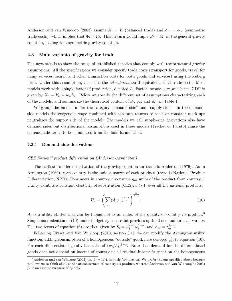
Anderson and van Wincoop (2003) assume Xi = Yi (balanced trade) and φni = φin (symmetric
trade costs), which implies that Φi = Ωi. This in turn would imply Si = Mi in the general gravity
equation, leading to a symmetric gravity equation.
2.3 Main variants of gravity for trade
The next step is to show the range of established theories that comply with the structural gravity
assumptions. All the specifications we consider specify trade costs (transport for goods, travel for
many services, search and other transaction costs for both goods and services) using the iceberg
form. Under this assumption, τni − 1 is the ad valorem tariff equivalent of all trade costs. Most
models work with a single factor of production, denoted L. Factor income is w, and hence GDP is
given by Xn = Yn = wnLn. Below we specify the different set of assumptions characterizing each
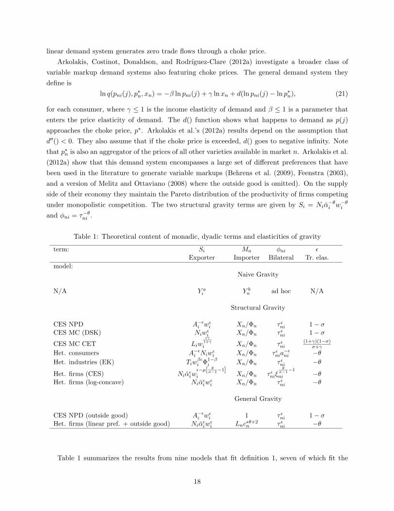
of the models, and summarize the theoretical content of Si, φni and Mn in Table 1.
We group the models under the category “demand-side” and “supply-side.” In the demand-
side models the exogenous wage combined with constant returns to scale or constant mark-ups
neutralizes the supply side of the model. The models we call supply-side derivations also have
demand sides but distributional assumptions used in these models (Frechet or Pareto) cause the
demand-side terms to be eliminated from the final formulation.
2.3.1 Demand-side derivations
CES National product differentiation (Anderson-Armington)
The earliest “modern” derivation of the gravity equation for trade is Anderson (1979). As in
Armington (1969), each country is the unique source of each product (there is National Product
Differentiation, NPD). Consumers in country n consume qni units of the product from country i.
Utility exhibits a constant elasticity of substitution (CES), σ > 1, over all the national products:
Un =
(∑i
(Aiqni)σ−1σ
) σσ−1
. (10)
Ai is a utility shifter that can be thought of as an index of the quality of country i’s product.8
Simple maximization of (10) under budgetary constraint provides optimal demand for each variety.
The two terms of equation (6) are then given by Si = Aσ−1i w1−σ
i , and φni = τ1−σni .
Following Okawa and Van Wincoop (2010, section 3.1), we can modify the Armington utility
function, adding consumption of a homogeneous “outside” good, here denoted q0n, to equation (10).
For each differentiated good i has sales of (wi/Ai)1−σ. Note that demand for the differentiated
goods does not depend on income of country n; all residual income is spent on the homogeneous
8Anderson and van Wincoop (2003) use βi = 1/Ai in their formulation. We prefer the one specified above becauseit allows us to think of Ai as the attractiveness of country i’s product, whereas Anderson and van Wincoop’s (2003)βi is an inverse measure of quality.
11

good. The resulting gravity equation still has Si = Aσ−1i w1−σ
i , and φni = τ1−σni but Mi = 1, because
Xn/Φn = 1 (assuming Xn corresponds to expenditures on the differentiated goods only). Adding
an outside good that enters utility linearly therefore leads to a specification that fits the general
definition for gravity but not the one we call “structural gravity.”9
CES Monopolistic competition (Dixit-Stiglitz-Krugman)
The gravity equation based on standard symmetric Dixit-Stiglitz-Krugman (DSK) monopolistic
competition assumptions was derived by multiple authors.10 It assumes that each country has Ni
firms supplying one variety each to the world from a home-country production site. Utility features
a constant elasticity of substitution, denoted σ, between all varieties available in the world. Dyadic
accessability is given by φni = τ1−σni . The exporter attribute is given by Si = Niw
1−σi , where the
difference compared to the NPD model is that the Ni term replaces Aσ−1i . Thus the exporter
attribute reflects the monopolistic competition among the symmetric varieties in the DSK model
and competitively supplied national varieties in the NPD model. Note that prices are also different
since they are a constant positive markup over marginal costs in DSK, and just equal to marginal
cost in NPD.
While the Dixit-Stiglitz model is usually interpreted as firms supplying differentiated goods
to consumers, the fact that the majority11 of trade involves intermediates suggests the benefits
of generalizing to that case. If we follow Ethier (1982) in assuming that each firm produces a
differentiated variety of intermediate input, the Si, Mn and φni terms remain the same.
CES demand with CET production
The earliest derivation of a gravity equation using monopolistic competition of the Dixit-Stiglitz
form is Bergstrand (1985). Bergstrand used a more general set of functional forms that were not
retained in later work (as described above). In particular, he allowed for a nested structure in which
domestic varieties are closer substitutes for each other than are foreign varieties. Bergstrand also
generalized the production side to allow for the possibility that output might not be transferable
to the export sector on a one-for-one basis. Instead he allows for a “constant elasticity of transfor-
mation” (CET). The idea is that output to one destination cannot be costlessly transformed into
output for a different destination. The elasticity of transformation is denoted γ and ranges from 0
where it is impossible to reallocate output to infinite, in which case transformation is costless.
Here we follow Baier and Bergstrand (2001) in assuming a finite CET, while retaining the
single-layer CES. This specification still yields structural gravity with
Si = Liwγ(1−σ)σ+γ
i and φni = τ(1+γ)(1−σ)
σ+γ
ni .
9This is an unfortunate aspect of the terminology but we could not find a suitable alternative.10One early derivation based on Krugman (1979) is contained in the unpublished paper of Wei (1996).11Chen et al. (2005) construct the share of intermediates in total trade for 10 OECD countries using input-output
tables in various years between 1968 and 1998. The US share averages 50% while the other countries have higheraverages, with Japan above 80% until the 1990s.
12
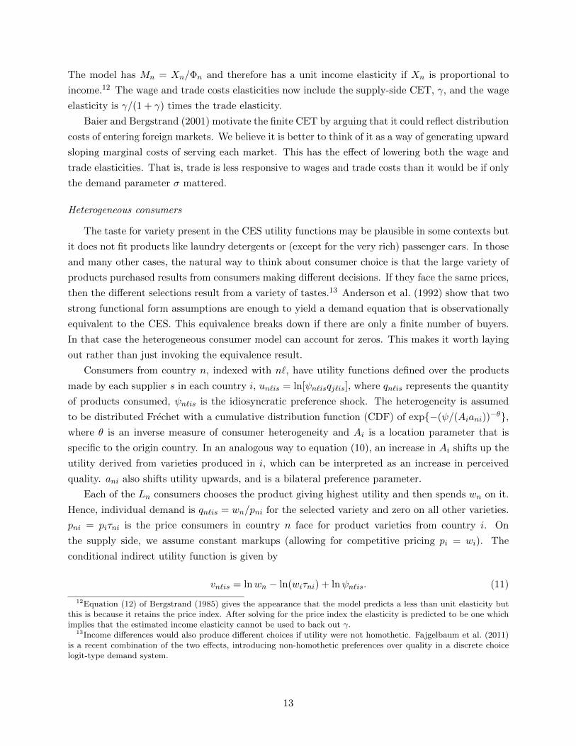
The model has Mn = Xn/Φn and therefore has a unit income elasticity if Xn is proportional to
income.12 The wage and trade costs elasticities now include the supply-side CET, γ, and the wage
elasticity is γ/(1 + γ) times the trade elasticity.
Baier and Bergstrand (2001) motivate the finite CET by arguing that it could reflect distribution
costs of entering foreign markets. We believe it is better to think of it as a way of generating upward
sloping marginal costs of serving each market. This has the effect of lowering both the wage and
trade elasticities. That is, trade is less responsive to wages and trade costs than it would be if only
the demand parameter σ mattered.
Heterogeneous consumers
The taste for variety present in the CES utility functions may be plausible in some contexts but
it does not fit products like laundry detergents or (except for the very rich) passenger cars. In those
and many other cases, the natural way to think about consumer choice is that the large variety of
products purchased results from consumers making different decisions. If they face the same prices,
then the different selections result from a variety of tastes.13 Anderson et al. (1992) show that two
strong functional form assumptions are enough to yield a demand equation that is observationally
equivalent to the CES. This equivalence breaks down if there are only a finite number of buyers.
In that case the heterogeneous consumer model can account for zeros. This makes it worth laying
out rather than just invoking the equivalence result.
Consumers from country n, indexed with n`, have utility functions defined over the products
made by each supplier s in each country i, un`is = ln[ψn`isqj`is], where qn`is represents the quantity
of products consumed, ψn`is is the idiosyncratic preference shock. The heterogeneity is assumed
to be distributed Frechet with a cumulative distribution function (CDF) of exp−(ψ/(Aiani))−θ,
where θ is an inverse measure of consumer heterogeneity and Ai is a location parameter that is
specific to the origin country. In an analogous way to equation (10), an increase in Ai shifts up the
utility derived from varieties produced in i, which can be interpreted as an increase in perceived
quality. ani also shifts utility upwards, and is a bilateral preference parameter.
Each of the Ln consumers chooses the product giving highest utility and then spends wn on it.
Hence, individual demand is qn`is = wn/pni for the selected variety and zero on all other varieties.
pni = piτni is the price consumers in country n face for product varieties from country i. On
the supply side, we assume constant markups (allowing for competitive pricing pi = wi). The
conditional indirect utility function is given by
vn`is = lnwn − ln(wiτni) + lnψn`is. (11)
12Equation (12) of Bergstrand (1985) gives the appearance that the model predicts a less than unit elasticity butthis is because it retains the price index. After solving for the price index the elasticity is predicted to be one whichimplies that the estimated income elasticity cannot be used to back out γ.
13Income differences would also produce different choices if utility were not homothetic. Fajgelbaum et al. (2011)is a recent combination of the two effects, introducing non-homothetic preferences over quality in a discrete choicelogit-type demand system.
13

The Frechet form for ψ implies a Gumbel form for lnψ and thereby implies multinomial logit forms
for the probabilities of choosing one of the Ni varieties produced in country i for consumers in n:
Pni =w−θi Aθi τ
−θni a
θni∑
`w−θ` Aθ`τ
−θn` a
θn`
. (12)
This equation has a second interpretation that applies to settings in which products are allocated to
consumers via auctions. Pni becomes the probability that i has the highest valuation and therefore
makes the winning bid for a good from n.14
Summing over the set of Ni varieties, E[πni] = NiPni. With a continuum of consumers, the
expectation is no longer needed, and πni = NiPni. This formulation meets the separability require-
ment of definition 2. The exporter attribute and the accessability terms are given by Si = Niw−θi Aθi ,
and φni = τ−θni aθni. The key difference in this model compared to the two former ones lies in the
parameter −θ substituting for 1 − σ when the demand system is CES. There is a very strong
parallel though, since an increase in σ means that products are becoming more homogenous, and
an increase in θ means that consumers are becoming less heterogenous. Whether consumers are
becoming more alike in their tastes, or whether products are becoming more substitutable yields
similar aggregate predictions for trade flows, which is quite intuitive.
Note that allowing for the bilateral shock ani to enter preferences of consumers makes it possible
for variables like distance to affect trade not only though freight costs, but also through preferences.
Another advantage of this model is that, for finite numbers of consumers in the importing country
n, it is possible for imports from i to have realized values of zero, an issue we return to in section 5.2.
2.3.2 Supply-side derivations
Heterogeneous Industries (Ricardian Comparative Advantage)
Eaton and Kortum (2002) derive a gravity equation that departs from the CES-based approaches
in almost every respect and yet the results they obtain bear a striking resemblance. In contrast
to the CES-NPD approach, each country produces a very large number of goods (modeled as a
continuum) that are homogeneous across countries. In contrast to the CES-MC approach, every
industry is perfectly competitive.15 Productivity z is assumed to be distributed Frechet with a
cumulative distribution function (CDF) of exp−Tiz−θ, where Ti is a technology parameter that
increases the share of goods for which i is the low-cost supplier and θ determines the amount of
heterogeneity in the productivity distribution. Note that the θ parameter now corresponds inversely
to dispersion in productivity rather than tastes. However, since this parameter plays the same key
role in both models, we maintain the notation in order to emphasize the similarity in resulting
terms.
14Hortacu et al. (2009) apply such a model to eBay transactions.15Bernard et al. (2003) reformulate the Eaton and Kortum (2002) model to allow for Bertrand competition in each
sector but this reformulation does not change the form of the gravity equation.
14
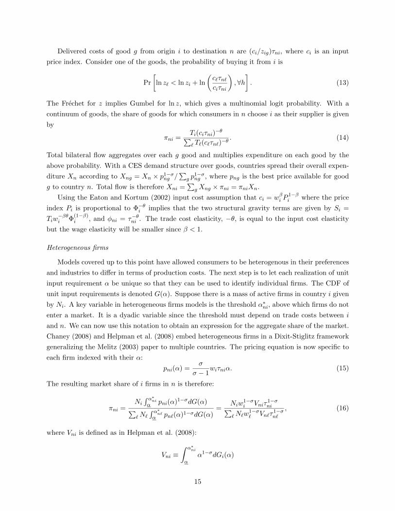
Delivered costs of good g from origin i to destination n are (ci/zig)τni, where ci is an input
price index. Consider one of the goods, the probability of buying it from i is
Pr
[ln z` < ln zi + ln
(c`τn`ciτni
),∀h]. (13)
The Frechet for z implies Gumbel for ln z, which gives a multinomial logit probability. With a
continuum of goods, the share of goods for which consumers in n choose i as their supplier is given
by
πni =Ti(ciτni)
−θ∑` T`(c`τn`)
−θ . (14)
Total bilateral flow aggregates over each g good and multiplies expenditure on each good by the
above probability. With a CES demand structure over goods, countries spread their overall expen-
diture Xn according to Xng = Xn × p1−σng /
∑g p
1−σng , where png is the best price available for good
g to country n. Total flow is therefore Xni =∑
gXng × πni = πniXn.
Using the Eaton and Kortum (2002) input cost assumption that ci = wβi P1−βi where the price
index Pi is proportional to Φ−θi implies that the two structural gravity terms are given by Si =
Tiw−βθi Φ
(1−β)i , and φni = τ−θni . The trade cost elasticity, −θ, is equal to the input cost elasticity
but the wage elasticity will be smaller since β < 1.
Heterogeneous firms
Models covered up to this point have allowed consumers to be heterogenous in their preferences
and industries to differ in terms of production costs. The next step is to let each realization of unit
input requirement α be unique so that they can be used to identify individual firms. The CDF of
unit input requirements is denoted G(α). Suppose there is a mass of active firms in country i given
by Ni. A key variable in heterogeneous firms models is the threshold α∗ni, above which firms do not
enter a market. It is a dyadic variable since the threshold must depend on trade costs between i
and n. We can now use this notation to obtain an expression for the aggregate share of the market.
Chaney (2008) and Helpman et al. (2008) embed heterogeneous firms in a Dixit-Stiglitz framework
generalizing the Melitz (2003) paper to multiple countries. The pricing equation is now specific to
each firm indexed with their α:
pni(α) =σ
σ − 1wiτniα. (15)
The resulting market share of i firms in n is therefore:
πni =Ni
∫ α∗niα pni(α)1−σdG(α)∑
`N`
∫ α∗n`α pn`(α)1−σdG(α)
=Niw
1−σi Vniτ
1−σni∑
`N`w1−σ` Vn`τ
1−σn`
, (16)
where Vni is defined as in Helpman et al. (2008):
Vni ≡∫ α∗ni
αα1−σdGi(α)
15

When the threshold entry costs, α∗ni, are less than the lower support, α, then Vni = 0 and there
will be no exports from i to n. To specify πni, we need to solve for Vni, and therefore to specify
α∗ni and Gi(α).
In this model, the equilibrium threshold α∗ni such that the corresponding firm is the last one to
serve market n (zero profit condition with fni the fixed cost of serving n from i) is
α∗ni = σσσ−1 (σ − 1)
(Xn
fniΦn
) 1σ−1 1
wiτni. (17)
Since α∗ni depends on destination country characteristics Xn and Φn, and on i-specific distribution
parameters in Gi(α), we generally cannot separate Vni multiplicatively as would be required to
obtain the structural form of gravity. The only functional form known to generate a multiplicable
closed form for Vni is the Pareto distribution. Hence we follow Helpman et al. (2008) in setting
Gi(α) = (αθ−αθ)/(αθi −αθ), where θ is the shape parameter and the support of input requirements
is α, αi. The lower bound of α > 0 is the mechanism through which Helpman et al. (2008) generate
aggregate bilateral trade flows of zero. However, to obtain the structural gravity form we need to
follow Chaney (2008) and Arkolakis et al. (2012b) in making zero the lower bound for α.16
Imposing Pareto (with α = 0 and country-specific αi) and solving for Vni, the aggregate market
share of i firms in n is
πni =Ni(wiαi)
−θτ−θni f−[ θ
σ−1−1]
ni∑`N`(w`αi)−θτ
−θn` f
−[ θσ−1−1]
n`
. (18)
The first point to note, made originally by Chaney (2008), is that the elasticity of trade with respect
to trade costs is now −θ a supply-side parameter, rather than 1−σ, the preference parameter that
determines the elasticity of trade for individual firms (and aggregate trade flows in symmetric firms
models). Both parameters can be interpreted as inverse measures of heterogeneity. However, while
dispersion in the consumer tastes are increasing in 1/(σ− 1), differences in productive efficiency of
firms are what rises with 1/θ. The disappearance of the demand parameter is purely a consequence
of the Pareto assumption, under which the elasticity of Vni with respect to trade costs is given by
−θ + σ − 1. When adding this elasticity to the intensive margin elasticity, the 1 − σ term drops
out.
Equation (18) shows that, in models with an extensive margin of firms’ entry, bilateral trade
is affected by both variable and fixed trade costs. Eaton et al. (2011a) use θ to denote θ/(σ − 1).
Since θ needs to be bigger than σ − 1 for the integral defined by Vni to be finite, θ > 1. Thus,
the elasticity of the trade with respect to bilateral fixed costs, −(θ − 1) is negative. The fixed
costs of entering markets may involve some costs incurred in the domestic economy, wi, as well
as costs incurred in the destination market, wn. Following Arkolakis et al. (2012b), we specify
16Since α is the inverse of productivity this means that productivity has no upper bound. In that case the continuumassumption implies positive mass of exporters for all country pairs ni.
16
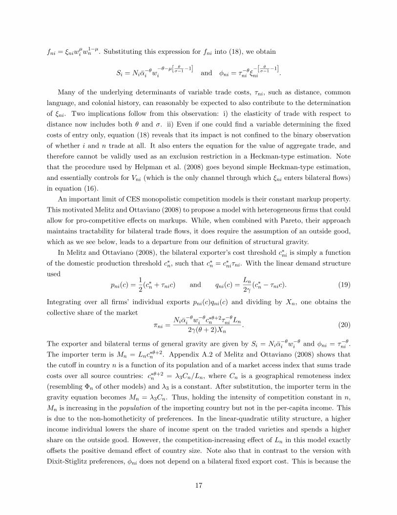
fni = ξniwµi w
1−µn . Substituting this expression for fni into (18), we obtain
Si = Niα−θi w
−θ−µ[ θσ−1−1]
i and φni = τ−θni ξ−[ θ
σ−1−1]
ni .
Many of the underlying determinants of variable trade costs, τni, such as distance, common
language, and colonial history, can reasonably be expected to also contribute to the determination
of ξni. Two implications follow from this observation: i) the elasticity of trade with respect to
distance now includes both θ and σ. ii) Even if one could find a variable determining the fixed
costs of entry only, equation (18) reveals that its impact is not confined to the binary observation
of whether i and n trade at all. It also enters the equation for the value of aggregate trade, and
therefore cannot be validly used as an exclusion restriction in a Heckman-type estimation. Note
that the procedure used by Helpman et al. (2008) goes beyond simple Heckman-type estimation,
and essentially controls for Vni (which is the only channel through which ξni enters bilateral flows)
in equation (16).
An important limit of CES monopolistic competition models is their constant markup property.
This motivated Melitz and Ottaviano (2008) to propose a model with heterogeneous firms that could
allow for pro-competitive effects on markups. While, when combined with Pareto, their approach
maintains tractability for bilateral trade flows, it does require the assumption of an outside good,
which as we see below, leads to a departure from our definition of structural gravity.
In Melitz and Ottaviano (2008), the bilateral exporter’s cost threshold c∗ni is simply a function
of the domestic production threshold c∗n, such that c∗n = c∗niτni. With the linear demand structure
used
pni(c) =1
2(c∗n + τnic) and qni(c) =
Ln2γ
(c∗n − τnic). (19)
Integrating over all firms’ individual exports pni(c)qni(c) and dividing by Xn, one obtains the
collective share of the market
πni =Niα
−θi w−θi c∗θ+2
n τ−θni Ln2γ(θ + 2)Xn
. (20)
The exporter and bilateral terms of general gravity are given by Si = Niα−θi w−θi and φni = τ−θni .
The importer term is Mn = Lnc∗θ+2n . Appendix A.2 of Melitz and Ottaviano (2008) shows that
the cutoff in country n is a function of its population and of a market access index that sums trade
costs over all source countries: c∗θ+2n = λ3Cn/Ln, where Cn is a geographical remoteness index
(resembling Φn of other models) and λ3 is a constant. After substitution, the importer term in the
gravity equation becomes Mn = λ3Cn. Thus, holding the intensity of competition constant in n,
Mn is increasing in the population of the importing country but not in the per-capita income. This
is due to the non-homotheticity of preferences. In the linear-quadratic utility structure, a higher
income individual lowers the share of income spent on the traded varieties and spends a higher
share on the outside good. However, the competition-increasing effect of Ln in this model exactly
offsets the positive demand effect of country size. Note also that in contrast to the version with
Dixit-Stiglitz preferences, φni does not depend on a bilateral fixed export cost. This is because the
17
linear demand system generates zero trade flows through a choke price.
Arkolakis, Costinot, Donaldson, and Rodrıguez-Clare (2012a) investigate a broader class of
variable markup demand systems also featuring choke prices. The general demand system they
define is
ln q(pni(j), p∗n, xn) = −β ln pni(j) + γ lnxn + d(ln pni(j)− ln p∗n), (21)
for each consumer, where γ ≤ 1 is the income elasticity of demand and β ≤ 1 is a parameter that
enters the price elasticity of demand. The d() function shows what happens to demand as p(j)
approaches the choke price, p∗. Arkolakis et al.’s (2012a) results depend on the assumption that
d′′() < 0. They also assume that if the choke price is exceeded, d() goes to negative infinity. Note
that p∗n is also an aggregator of the prices of all other varieties available in market n. Arkolakis et al.
(2012a) show that this demand system encompasses a large set of different preferences that have
been used in the literature to generate variable markups (Behrens et al. (2009), Feenstra (2003),
and a version of Melitz and Ottaviano (2008) where the outside good is omitted). On the supply
side of their economy they maintain the Pareto distribution of the productivity of firms competing
under monopolistic competition. The two structural gravity terms are given by Si = Niα−θi w−θi
and φni = τ−θni .
Table 1: Theoretical content of monadic, dyadic terms and elasticities of gravity
term: Si Mn φni εExporter Importer Bilateral Tr. elas.
model:Naive Gravity
N/A Y ai Y b
n ad hoc N/A
Structural Gravity
CES NPD A−εi wεi Xn/Φn τ εni 1− σCES MC (DSK) Niw
εi Xn/Φn τ εni 1− σ
CES MC CET Liwεγ
1+γ
i Xn/Φn τ εni(1+γ)(1−σ)
σ+γ
Het. consumers A−εi Niwεi Xn/Φn τ εnia
−εni −θ
Het. industries (EK) Tiwβεi Φ1−β
i Xn/Φn τ εni −θ
Het. firms (CES) Niαεiw
ε−µ[ θσ−1−1]
i Xn/Φn τ εniξθ
σ−1−1
ni −θHet. firms (log-concave) Niα
εiw
εi Xn/Φn τ εni −θ
General Gravity
CES NPD (outside good) A−εi wεi 1 τ εni 1− σHet. firms (linear pref. + outside good) Niα
εiw
εi Lnc
∗θ+2n τ εni −θ
Table 1 summarizes the results from nine models that fit definition 1, seven of which fit the
18

stronger requirements of definition 2. The final column shows trade elasticities with respect to
variable trade costs, ε. Note that in most structural gravity models, the elasticity of trade with
respect to wages is also given by ε. For CES-CET, this occurs in the limit as γ →∞ (reallocation
of output across destination is costless), for heterogeneous industries it occurs as β → 1 (labor
is the only input) and for heterogenous firms as µ → 0 (fixed costs is paid in units of foreign
labor). In principle, if one had reliable estimates of both wage and trade elasticities, one could
infer something about these parameters. An important difficulty is to find good instruments for
cross-country variation in wages of the origin country that can be excluded from the trade equation.
2.4 Gravity models beyond trade in goods
The same modeling tools that yield gravity equations for trade in goods can also be applied to other
types of flows and interactions. Head et al. (2009) adapt the Eaton and Kortum (2002) model to
the case of service offshoring. Anderson (2011) presents a migration gravity model drawing on
discrete choice techniques. Ahlfeldt et al. (2012) draw on Eaton and Kortum (2002) to specify a
commuting gravity model. With a few minor changes, the discrete choice framework can easily
produce a gravity equation for tourism.
Portes et al. (2001) and Portes and Rey (2005) establish that gravity equations (“naive” defi-
nition) can explain cross border portfolio investment patterns as well as they explain trade flows.
Martin and Rey (2004) propose a 2-country model that they use to justify a gravity equation for
bilateral portfolio investment. Coeurdacier and Martin (2009) generalize the framework to multiple
countries and apply it using different types of assets and a fixed effects estimation technology very
close to the one used by trade economists. Okawa and van Wincoop (2012) suggest an alternative
foundation for gravity in international finance.
Gravity equations have also been shown to do a good job fitting stocks of foreign direct invest-
ment (FDI). Head and Ries (2008) consider a model in which FDI takes the form of acquisitions.
Using the discrete choice framework in a way that resembles Eaton and Kortum (2002), they de-
velop a gravity equation for FDI which fits the data well. de Sousa and Lochard (2011) extend the
model to greenfield investment by imagining that instead of bidding for assets, each corporation
selects the best “investment project” across all host countries.
In summary, one of the contributions of the development of micro-foundations for the gravity
equation for trade is that they can be applied to a range of other bilateral flows and interactions.
The key ingredients tend to be “mass” effects that come from adding up constraints and bilateral
and multilateral “resistance” terms. Once these gravity equations are specified, they can usually
be estimated using the same techniques that are appropriate for trade flows.
3 Theory-consistent estimation
After having described the different theoretical setups that give rise to the gravity prediction, we
turn to estimation methods that are consistent with the theory predictions, in particular because
19
they do account for the multilateral resistance terms that are a key feature of general and structural
gravity. Historically, the very first approach was to proxy multilateral resistance with remoteness
terms. This approached progressively appeared as too weak once the theoretical modeling of grav-
ity became clearer. Researchers then switched to more structural approaches. Because of the
influence of Anderson and van Wincoop (2003) in the literature, we start with a version of their
approach (their original approach using non-linear least squares has actually been hardly followed),
that applies the full structure of the structural gravity framework. We then describe fixed effects
estimation that imposes much less structure, but still complies with general gravity. This method
can however encounter computational difficulties when using very large datasets, which is not un-
common in the literature. We therefore turn to alternatives when fixed effects are not feasible, and
end with Monte Carlo comparisons of all those methods.
3.1 Proxies for multilateral resistance terms
A few early studies have included variables proxies for 1/Ωi and 1/Φn and referred to them as “re-
moteness.” Wei (1996) used a monopolistic competition model to show the theoretical counterparts
of these variables but settled for using “log(GDP)-weighted average distances” in his regressions.17
This bears little resemblance to its theoretical counterpart. Some other remoteness measures differ
from their theoretical counterparts in ways that are even more problematic. For instance, Helliwell
(1998) measures remoteness as REM1n =∑
i Distni/Yi. This measure has the feature of giving
extraordinary weight to tiny countries: as Yi → 0, REM1 explodes. A better measure of remoteness
is REM2n = (∑
i Yi/Distni)−1, that is the inverse of the Harris market potential.18 Tiny countries
have negligible effects on REM2 and the size of very distant countries becomes irrelevant. Supposing
φni ∼ Dist−1ni and Xn = Yn, the correct Φn and Ωi are
∑`(Y`/Distn`)Ω
−1` and
∑`(Y`/Distn`)Φ
−1` .
Thus we see that REM2 is on the right track by summing up GDP to distance ratios but it ends
up wide off the mark because it implicitly assumes that Φ` and Ω` equal one. This makes no sense
when the whole point is to obtain a proxy for those variables. Furthermore, while Dist−1ni is an
important factor in determining φni many other trade costs besides distance ought to be considered.
In sum, proxy variables do not take the theory seriously enough, a concern that underlines the need
for gravitas.
3.2 Iterative structural estimation
Our implementation of the Anderson and van Wincoop (2003) method involves assuming initial
values of Ωi = 1 and Φn = 1, then estimating the vector of parameters determining φni, then using a
contraction mapping algorithm to find fixed points for Ωi and Φn given those parameters. We then
run OLS using lnXni− lnYi− lnXn+ln Ωi+ln Φni as the dependent variable. This gives a new set
17It is interesting to note that the literature has kept “circling” around those GDP-weighted averages of trade costsas proxies for the MR terms. Baier and Bergstrand (2009), discussed below, can be viewed as the latest approach inthat tradition, but one that maintains a clear connection (via approximation) back to the model.
18Baldwin and Harrigan (2011) use REM2 to explain the bilateral zero trade flows and Martin et al. (2008) usesomething close to REM2 as an instrument for trade.
20
of φni parameter estimates. We iterate until the parameter estimates stop changing. This method
exploits the structural relationship between Ωi, Φn, and φni. We therefore call the estimator SILS
(structurally iterated least squares). Although it is not identical to the Anderson and van Wincoop
(2003) method—which is estimated using a non-linear least squares routine in Gauss—SILS does
have the advantage of being available as a Stata ado file (available on our companion website). On
the other hand, while SILS uses OLS only, the iteration is time-consuming. Also, the structural
methods require data on trade with self and distance to self, both of which may be problematic.
3.3 Fixed effects estimation
Standard estimating procedure involves taking logs of equation (1), obtaining
lnXni = lnG+ lnSi + lnMn + lnφni. (22)
The naive form of gravity equations involved using log GDPs (and possibly other variables) as
proxies for the lnSi and lnMn but modern practice has been moving towards using fixed effects
for these terms instead (Harrigan (1996) seems to be the first paper to have done so). Note that
estimating gravity equations with fixed effects for the importer and exporter, as is now common
practice and recommended by major empirical trade economists, does not involve strong struc-
tural assumptions on the underlying model. As long as the precise modeling structure yields an
equation in multiplicative form such as (1), using fixed effects will yield consistent estimates of the
components of φni, which are usually the items of primary interest.19
We focus the exposition and our Monte Carlo investigation on cross-sections. However, most
current gravity estimations employ data sets that span many years. In such cases the importer and
exporter fixed effects should by time-varying as well. The same is true if the data pools over several
industries. The Si and Mn have no reason to be identical across industries since supply capacity
of i and total expenditure of n will vary across industries, because of differences in comparative
advantages or in consumer’s preferences for instance. For panels of trade flows with a large number
of years and/or industries, the estimation might run into computational feasability issues due to
the very large number of resulting dummies to be estimated, a challenge that now appears to be
solved, as we shall discuss below.
Using country fixed effects has an additional advantage that has nothing to do with being
consistent with theory. There can be systematic tendencies of a country to export large amounts
relative to its GDP and other observed trade determinants. As an example consider Netherlands
and Belgium. Much of Europe’s trade flows through Rotterdam and Antwerp. In principle the
production location should be used as the exporting country and the consumption location as the
importing country. In practice use of warehouses and other reporting issues makes this difficult
so there is reason to expect that trade flows to and from these countries are over-stated. Fixed
19Although the particular model underlying the fixed effects does not matter for the φni coefficients, it does affectthe mapping from the Si and Mn estimates back to primitives such as technology or demand parameters.
21
effects can control for this, since they will account for any unobservable that contributes to shift
the overall level of exports or imports of a country.
3.4 Ratio-type estimation
As mentioned above, the use of fixed effects can sometimes hit a computational constraint imposed
upon the number of separate parameters that can be estimated by a statistical package. A solution
that has been explored involves using the multiplicative structure of the gravity model to eliminate
the monadic terms, Si and Mn. Head and Mayer (2000) and Eaton and Kortum (2002) normalize
bilateral flows Xni by trade with self20 (Xnn) for a given industry/year, delivering a ratio we call
the odds specification:Xni
Xnn=
(SiSn
)(φniφnn
). (23)
While this specification simplifies greatly the issue by removing any characteristic of the importer,
the origin country term S remains to be measured, presumably with substantial error. A related
issue is that constructing Si requires knowledge of the trade cost elasticity, which is also contained
in the φni to be estimated through (23).
Head and Ries (2001) propose a simple solution to cancel those exporter terms, multiplying (23)
by XinXii
. If one is ready to assume symmetry in bilateral trade costs (φni = φin), and frictionless
trade inside countries (φnn = φii = 1), we end up with a very simple index that Eaton et al. (2011b)
call the Head-Ries Index (HRI),
φni =
√XniXin
XnnXii, (24)
and which can be used to assess the overall level of trade integration between any two countries.21
The problem with the HRI is that it cannot be calculated without a measure of trade inside
a country (Xnn). In principle, it can be proxied using production minus total exports of a coun-
try/industry/year combination. Disturbingly, this procedure generates some negative observations,
notably for countries like Belgium and the Netherlands, pointing to potential measurement issues
related, in particular, to transit shipments, as stated above. Alternative, but related, solutions exist
that omit the need for internal trade. Romalis (2007) and Hallak (2006) have used ratios of ratios
methods, involving four different international trade flows and thus named the Tetrads method by
Head et al. (2010). Choosing a reference importer k and a reference exporter `, provides a tetradic
term such thatXni/Xki
Xn`/Xk`=φni/φkiφn`/φk`
. (25)
20Those manipulations can be done with a reference country other than self. Martin et al. (2008) and Andersonand Marcouiller (2002) use the United States as the reference country.
21Head and Ries (2001) apply it to US/Canada free trade agreement, Head and Mayer (2004a) to a comparisonof North American and European integration, Jacks et al. (2008) use it to measure trade integration over the verylong run using trade data of France, Germany and the UK from 1870 to 2000, and Eaton et al. (2011b) use it toquantify the effects of the 2008-2009 crisis on trade integration. φni can also be used as the LHS of a regressiontrying to explain the bilateral determinants of trade integration (Combes et al. (2005), and Chen and Novy (2011)are examples following that path).
22
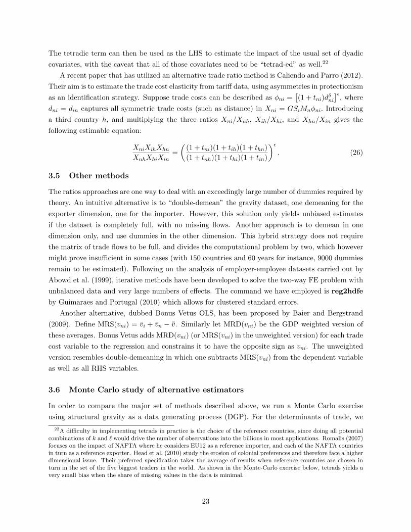
The tetradic term can then be used as the LHS to estimate the impact of the usual set of dyadic
covariates, with the caveat that all of those covariates need to be “tetrad-ed” as well.22
A recent paper that has utilized an alternative trade ratio method is Caliendo and Parro (2012).
Their aim is to estimate the trade cost elasticity from tariff data, using asymmetries in protectionism
as an identification strategy. Suppose trade costs can be described as φni =[(1 + tni)d
δni
]ε, where
dni = din captures all symmetric trade costs (such as distance) in Xni = GSiMnφni. Introducing
a third country h, and multiplying the three ratios Xni/Xnh, Xih/Xhi, and Xhn/Xin gives the
following estimable equation:
XniXihXhn
XnhXhiXin=
((1 + tni)(1 + tih)(1 + thn)
(1 + tnh)(1 + thi)(1 + tin)
)ε. (26)
3.5 Other methods
The ratios approaches are one way to deal with an exceedingly large number of dummies required by
theory. An intuitive alternative is to “double-demean” the gravity dataset, one demeaning for the
exporter dimension, one for the importer. However, this solution only yields unbiased estimates
if the dataset is completely full, with no missing flows. Another approach is to demean in one
dimension only, and use dummies in the other dimension. This hybrid strategy does not require
the matrix of trade flows to be full, and divides the computational problem by two, which however
might prove insufficient in some cases (with 150 countries and 60 years for instance, 9000 dummies
remain to be estimated). Following on the analysis of employer-employee datasets carried out by
Abowd et al. (1999), iterative methods have been developed to solve the two-way FE problem with
unbalanced data and very large numbers of effects. The command we have employed is reg2hdfe
by Guimaraes and Portugal (2010) which allows for clustered standard errors.
Another alternative, dubbed Bonus Vetus OLS, has been proposed by Baier and Bergstrand
(2009). Define MRS(vni) = vi + vn − ¯v. Similarly let MRD(vni) be the GDP weighted version of
these averages. Bonus Vetus adds MRD(vni) (or MRS(vni) in the unweighted version) for each trade
cost variable to the regression and constrains it to have the opposite sign as vni. The unweighted
version resembles double-demeaning in which one subtracts MRS(vni) from the dependent variable
as well as all RHS variables.
3.6 Monte Carlo study of alternative estimators
In order to compare the major set of methods described above, we run a Monte Carlo exercise
using structural gravity as a data generating process (DGP). For the determinants of trade, we
22A difficulty in implementing tetrads in practice is the choice of the reference countries, since doing all potentialcombinations of k and ` would drive the number of observations into the billions in most applications. Romalis (2007)focuses on the impact of NAFTA where he considers EU12 as a reference importer, and each of the NAFTA countriesin turn as a reference exporter. Head et al. (2010) study the erosion of colonial preferences and therefore face a higherdimensional issue. Their preferred specification takes the average of results when reference countries are chosen inturn in the set of the five biggest traders in the world. As shown in the Monte-Carlo exercise below, tetrads yields avery small bias when the share of missing values in the data is minimal.
23
use actual data for the 170 countries for which we have data on GDP, distance, and the existence
of a Regional Trade Agreement (RTA) in 2006. The DGP specifies accessibility as a function of
distance and RTA:
φni = exp(− ln Distni + 0.5RTAni)ηni,
where ηni is a log-normal random term. The ηni is the only stochastic term in the simulation since
the GDPs, distances, and RTA relationships are all set by actual data. We calibrate the variance
of ln ηni to replicate the RMSE of the LSDV regression on real data. As we will show later,
the distance elasticity of −1 and the 0.5 coefficient on the RTA dummy are representative of the
literature. Combining this with incomes of exporters and importers, we calculate the multilateral
resistance terms, Φn and Ωi using equation (3), which are used in (2) to generate bilateral trade
flows.23
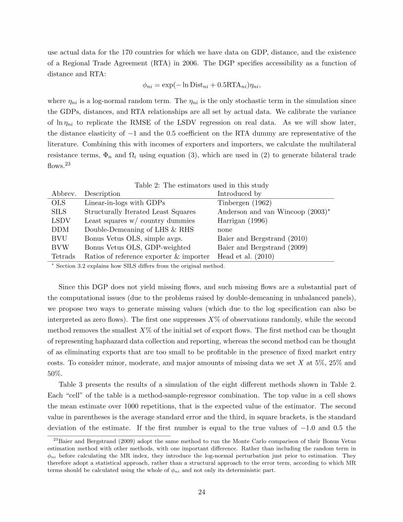
Table 2: The estimators used in this studyAbbrev. Description Introduced by
OLS Linear-in-logs with GDPs Tinbergen (1962)SILS Structurally Iterated Least Squares Anderson and van Wincoop (2003)∗
LSDV Least squares w/ country dummies Harrigan (1996)DDM Double-Demeaning of LHS & RHS noneBVU Bonus Vetus OLS, simple avgs. Baier and Bergstrand (2010)BVW Bonus Vetus OLS, GDP-weighted Baier and Bergstrand (2009)Tetrads Ratios of reference exporter & importer Head et al. (2010)∗ Section 3.2 explains how SILS differs from the original method.
Since this DGP does not yield missing flows, and such missing flows are a substantial part of
the computational issues (due to the problems raised by double-demeaning in unbalanced panels),
we propose two ways to generate missing values (which due to the log specification can also be
interpreted as zero flows). The first one suppresses X% of observations randomly, while the second
method removes the smallest X% of the initial set of export flows. The first method can be thought
of representing haphazard data collection and reporting, whereas the second method can be thought
of as eliminating exports that are too small to be profitable in the presence of fixed market entry
costs. To consider minor, moderate, and major amounts of missing data we set X at 5%, 25% and
50%.
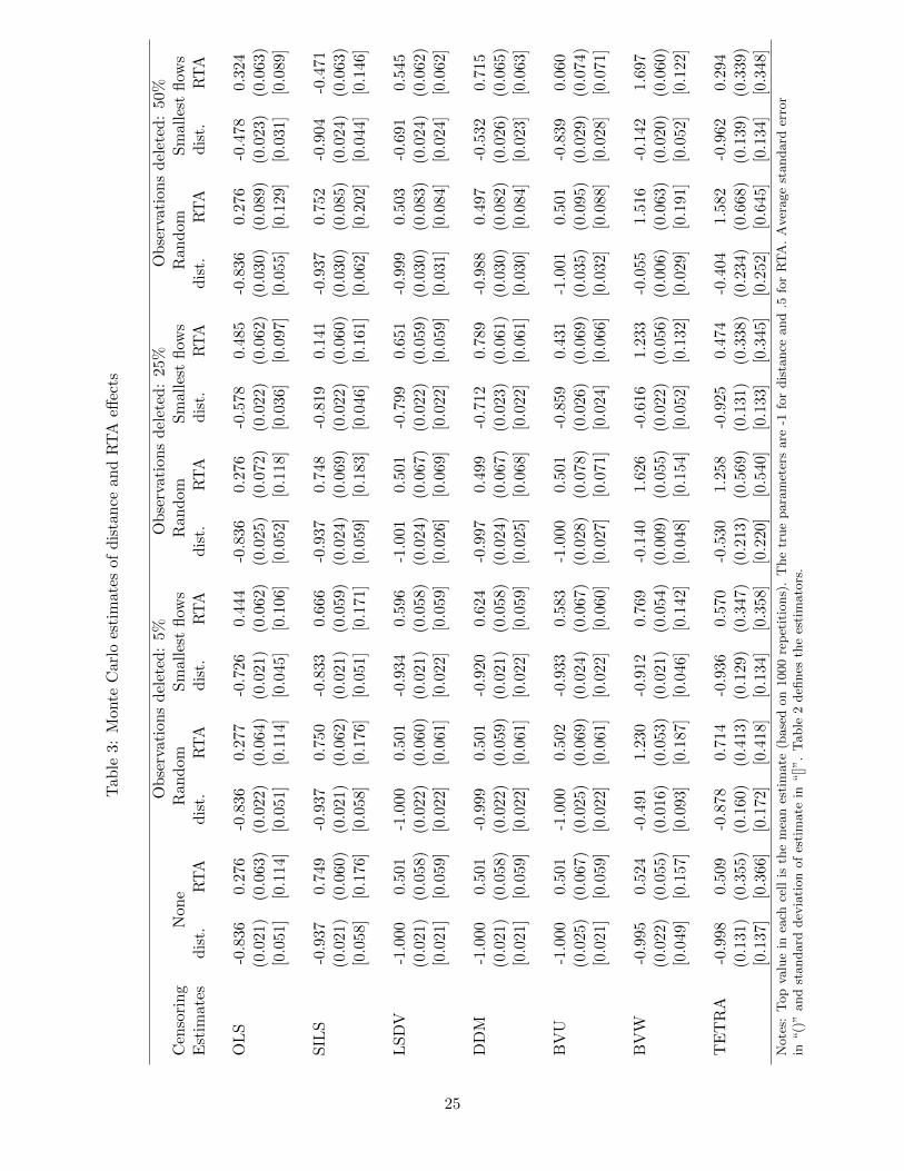
Table 3 presents the results of a simulation of the eight different methods shown in Table 2.
Each “cell” of the table is a method-sample-regressor combination. The top value in a cell shows
the mean estimate over 1000 repetitions, that is the expected value of the estimator. The second
value in parentheses is the average standard error and the third, in square brackets, is the standard
deviation of the estimate. If the first number is equal to the true values of −1.0 and 0.5 the
23Baier and Bergstrand (2009) adopt the same method to run the Monte Carlo comparison of their Bonus Vetusestimation method with other methods, with one important difference. Rather than including the random term inφni before calculating the MR index, they introduce the log-normal perturbation just prior to estimation. Theytherefore adopt a statistical approach, rather than a structural approach to the error term, according to which MRterms should be calculated using the whole of φni and not only its deterministic part.
24
Tab
le3:
Mon
teC
arlo
esti
mat
esof
dis
tan
cean
dR
TA
effec
ts
Ob
serv
atio
ns
del
eted
:5%
Ob
serv
atio
ns
del
eted
:25
%O
bse
rvat
ion
sd
elet
ed:
50%
Cen
sori
ng
Non
eR
and
omSm
alle
stfl
ows
Ran
dom
Sm
alle
stfl
ows
Ran
dom
Sm
alle
stflow
sE
stim
ate
sd
ist.
RT
Ad
ist.
RT
Ad
ist.
RT
Ad
ist.
RT
Ad
ist.
RT
Ad
ist.
RT
Ad
ist.
RT
A
OL
S-0
.836
0.2
76-0
.836
0.27
7-0
.726
0.44
4-0
.836
0.27
6-0
.578
0.48
5-0
.836
0.27
6-0
.478
0.32
4(0
.021
)(0
.063
)(0
.022)
(0.0
64)
(0.0
21)
(0.0
62)
(0.0
25)
(0.0
72)
(0.0
22)
(0.0
62)
(0.0
30)
(0.0
89)
(0.0
23)
(0.0
63)
[0.0
51]
[0.1
14]
[0.0
51]
[0.1
14]
[0.0
45]
[0.1
06]
[0.0
52]
[0.1
18]
[0.0
36]
[0.0
97]
[0.0
55]
[0.1
29]
[0.0
31]
[0.0
89]
SIL
S-0
.937
0.7
49-0
.937
0.75
0-0
.833
0.66
6-0
.937
0.74
8-0
.819
0.14
1-0
.937
0.75
2-0
.904
-0.4
71(0
.021
)(0
.060
)(0
.021)
(0.0
62)
(0.0
21)
(0.0
59)
(0.0
24)
(0.0
69)
(0.0
22)
(0.0
60)
(0.0
30)
(0.0
85)
(0.0
24)
(0.0
63)
[0.0
58]
[0.1
76]
[0.0
58]
[0.1
76]
[0.0
51]
[0.1
71]
[0.0
59]
[0.1
83]
[0.0
46]
[0.1
61]
[0.0
62]
[0.2
02]
[0.0
44]
[0.1
46]
LS
DV
-1.0
000.5
01-1
.000
0.50
1-0
.934
0.59
6-1
.001
0.50
1-0
.799
0.65
1-0
.999
0.50
3-0
.691
0.54
5(0
.021
)(0
.058
)(0
.022)
(0.0
60)
(0.0
21)
(0.0
58)
(0.0
24)
(0.0
67)
(0.0
22)
(0.0
59)
(0.0
30)
(0.0
83)
(0.0
24)
(0.0
62)
[0.0
21]
[0.0
59]
[0.0
22]
[0.0
61]
[0.0
22]
[0.0
59]
[0.0
26]
[0.0
69]
[0.0
22]
[0.0
59]
[0.0
31]
[0.0
84]
[0.0
24]
[0.0
62]
DD
M-1
.000
0.5
01-0
.999
0.50
1-0
.920
0.62
4-0
.997
0.49
9-0
.712
0.78
9-0
.988
0.49
7-0
.532
0.71
5(0
.021
)(0
.058
)(0
.022)
(0.0
59)
(0.0
21)
(0.0
58)
(0.0
24)
(0.0
67)
(0.0
23)
(0.0
61)
(0.0
30)
(0.0
82)
(0.0
26)
(0.0
65)
[0.0
21]
[0.0
59]
[0.0
22]
[0.0
61]
[0.0
22]
[0.0
59]
[0.0
25]
[0.0
68]
[0.0
22]
[0.0
61]
[0.0
30]
[0.0
84]
[0.0
23]
[0.0
63]
BV
U-1
.000
0.5
01
-1.0
000.
502
-0.9
330.
583
-1.0
000.
501
-0.8
590.
431
-1.0
010.
501
-0.8
390.
060
(0.0
25)
(0.0
67)
(0.0
25)
(0.0
69)
(0.0
24)
(0.0
67)
(0.0
28)
(0.0
78)
(0.0
26)
(0.0
69)
(0.0
35)
(0.0
95)
(0.0
29)
(0.0
74)
[0.0
21]
[0.0
59]
[0.0
22]
[0.0
61]
[0.0
22]
[0.0
60]
[0.0
27]
[0.0
71]
[0.0
24]
[0.0
66]
[0.0
32]
[0.0
88]
[0.0
28]
[0.0
71]
BV
W-0
.995
0.52
4-0
.491
1.23
0-0
.912
0.76
9-0
.140
1.62
6-0
.616
1.23
3-0
.055
1.51
6-0
.142
1.69
7(0
.022
)(0
.055
)(0
.016)
(0.0
53)
(0.0
21)
(0.0
54)
(0.0
09)
(0.0
55)
(0.0
22)
(0.0
56)
(0.0
06)
(0.0
63)
(0.0
20)
(0.0
60)
[0.0
49]
[0.1
57]
[0.0
93]
[0.1
87]
[0.0
46]
[0.1
42]
[0.0
48]
[0.1
54]
[0.0
52]
[0.1
32]
[0.0
29]
[0.1
91]
[0.0
52]
[0.1
22]
TE
TR
A-0
.998
0.50
9-0
.878
0.7
14-0
.936
0.57
0-0
.530
1.25
8-0
.925
0.47
4-0
.404
1.58
2-0
.962
0.29
4(0
.131
)(0
.355
)(0
.160)
(0.4
13)
(0.1
29)
(0.3
47)
(0.2
13)
(0.5
69)
(0.1
31)
(0.3
38)
(0.2
34)
(0.6
68)
(0.1
39)
(0.3
39)
[0.1
37]
[0.3
66]
[0.1
72]
[0.4
18]
[0.1
34]
[0.3
58]
[0.2
20]
[0.5
40]
[0.1
33]
[0.3
45]
[0.2
52]
[0.6
45]
[0.1
34]
[0.3
48]
Note
s:T
op
valu
ein
each
cell
isth
em
ean
esti
mate
(base
don
1000
rep
etit
ions)
.T
he
true
para
met
ers
are
-1fo
rdis
tance
and
.5fo
rR
TA
.A
ver
age
standard
erro
rin
“()
”and
standard
dev
iati
on
of
esti
mate
in“[]”.
Table
2defi
nes
the
esti
mato
rs.
25
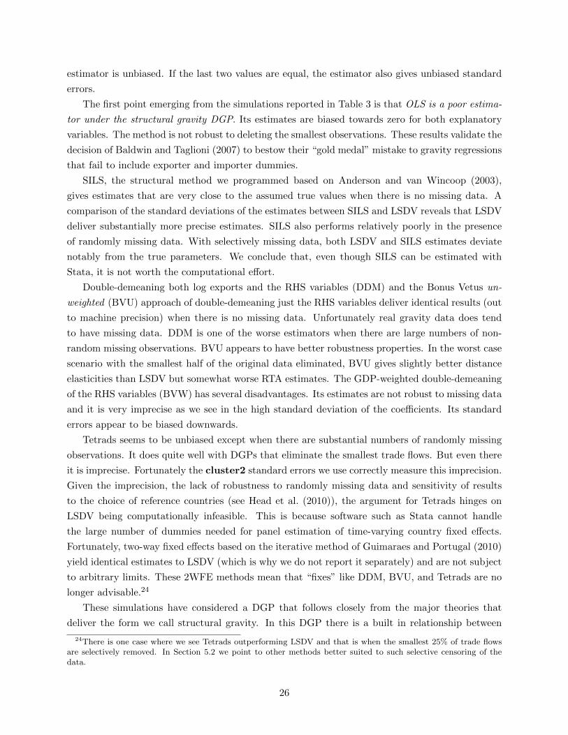
estimator is unbiased. If the last two values are equal, the estimator also gives unbiased standard
errors.
The first point emerging from the simulations reported in Table 3 is that OLS is a poor estima-
tor under the structural gravity DGP. Its estimates are biased towards zero for both explanatory
variables. The method is not robust to deleting the smallest observations. These results validate the
decision of Baldwin and Taglioni (2007) to bestow their “gold medal” mistake to gravity regressions
that fail to include exporter and importer dummies.
SILS, the structural method we programmed based on Anderson and van Wincoop (2003),
gives estimates that are very close to the assumed true values when there is no missing data. A
comparison of the standard deviations of the estimates between SILS and LSDV reveals that LSDV
deliver substantially more precise estimates. SILS also performs relatively poorly in the presence
of randomly missing data. With selectively missing data, both LSDV and SILS estimates deviate
notably from the true parameters. We conclude that, even though SILS can be estimated with
Stata, it is not worth the computational effort.
Double-demeaning both log exports and the RHS variables (DDM) and the Bonus Vetus un-
weighted (BVU) approach of double-demeaning just the RHS variables deliver identical results (out
to machine precision) when there is no missing data. Unfortunately real gravity data does tend
to have missing data. DDM is one of the worse estimators when there are large numbers of non-
random missing observations. BVU appears to have better robustness properties. In the worst case
scenario with the smallest half of the original data eliminated, BVU gives slightly better distance
elasticities than LSDV but somewhat worse RTA estimates. The GDP-weighted double-demeaning
of the RHS variables (BVW) has several disadvantages. Its estimates are not robust to missing data
and it is very imprecise as we see in the high standard deviation of the coefficients. Its standard
errors appear to be biased downwards.
Tetrads seems to be unbiased except when there are substantial numbers of randomly missing
observations. It does quite well with DGPs that eliminate the smallest trade flows. But even there
it is imprecise. Fortunately the cluster2 standard errors we use correctly measure this imprecision.
Given the imprecision, the lack of robustness to randomly missing data and sensitivity of results
to the choice of reference countries (see Head et al. (2010)), the argument for Tetrads hinges on
LSDV being computationally infeasible. This is because software such as Stata cannot handle
the large number of dummies needed for panel estimation of time-varying country fixed effects.
Fortunately, two-way fixed effects based on the iterative method of Guimaraes and Portugal (2010)
yield identical estimates to LSDV (which is why we do not report it separately) and are not subject
to arbitrary limits. These 2WFE methods mean that “fixes” like DDM, BVU, and Tetrads are no
longer advisable.24
These simulations have considered a DGP that follows closely from the major theories that
deliver the form we call structural gravity. In this DGP there is a built in relationship between
24There is one case where we see Tetrads outperforming LSDV and that is when the smallest 25% of trade flowsare selectively removed. In Section 5.2 we point to other methods better suited to such selective censoring of thedata.
26
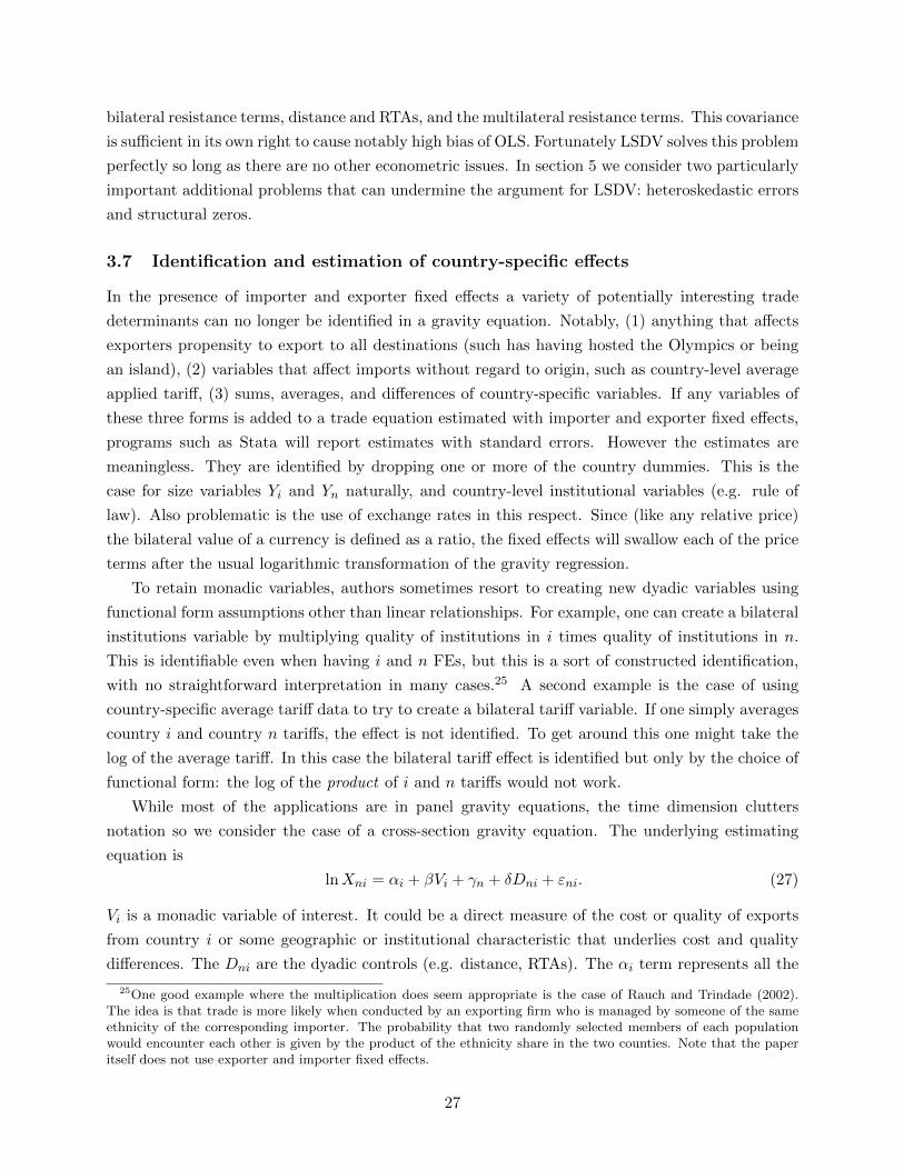
bilateral resistance terms, distance and RTAs, and the multilateral resistance terms. This covariance
is sufficient in its own right to cause notably high bias of OLS. Fortunately LSDV solves this problem
perfectly so long as there are no other econometric issues. In section 5 we consider two particularly
important additional problems that can undermine the argument for LSDV: heteroskedastic errors
and structural zeros.
3.7 Identification and estimation of country-specific effects
In the presence of importer and exporter fixed effects a variety of potentially interesting trade
determinants can no longer be identified in a gravity equation. Notably, (1) anything that affects
exporters propensity to export to all destinations (such has having hosted the Olympics or being
an island), (2) variables that affect imports without regard to origin, such as country-level average
applied tariff, (3) sums, averages, and differences of country-specific variables. If any variables of
these three forms is added to a trade equation estimated with importer and exporter fixed effects,
programs such as Stata will report estimates with standard errors. However the estimates are
meaningless. They are identified by dropping one or more of the country dummies. This is the
case for size variables Yi and Yn naturally, and country-level institutional variables (e.g. rule of
law). Also problematic is the use of exchange rates in this respect. Since (like any relative price)
the bilateral value of a currency is defined as a ratio, the fixed effects will swallow each of the price
terms after the usual logarithmic transformation of the gravity regression.
To retain monadic variables, authors sometimes resort to creating new dyadic variables using
functional form assumptions other than linear relationships. For example, one can create a bilateral
institutions variable by multiplying quality of institutions in i times quality of institutions in n.
This is identifiable even when having i and n FEs, but this is a sort of constructed identification,
with no straightforward interpretation in many cases.25 A second example is the case of using
country-specific average tariff data to try to create a bilateral tariff variable. If one simply averages
country i and country n tariffs, the effect is not identified. To get around this one might take the
log of the average tariff. In this case the bilateral tariff effect is identified but only by the choice of
functional form: the log of the product of i and n tariffs would not work.
While most of the applications are in panel gravity equations, the time dimension clutters
notation so we consider the case of a cross-section gravity equation. The underlying estimating
equation is
lnXni = αi + βVi + γn + δDni + εni. (27)
Vi is a monadic variable of interest. It could be a direct measure of the cost or quality of exports
from country i or some geographic or institutional characteristic that underlies cost and quality
differences. The Dni are the dyadic controls (e.g. distance, RTAs). The αi term represents all the
25One good example where the multiplication does seem appropriate is the case of Rauch and Trindade (2002).The idea is that trade is more likely when conducted by an exporting firm who is managed by someone of the sameethnicity of the corresponding importer. The probability that two randomly selected members of each populationwould encounter each other is given by the product of the ethnicity share in the two counties. Note that the paperitself does not use exporter and importer fixed effects.
27
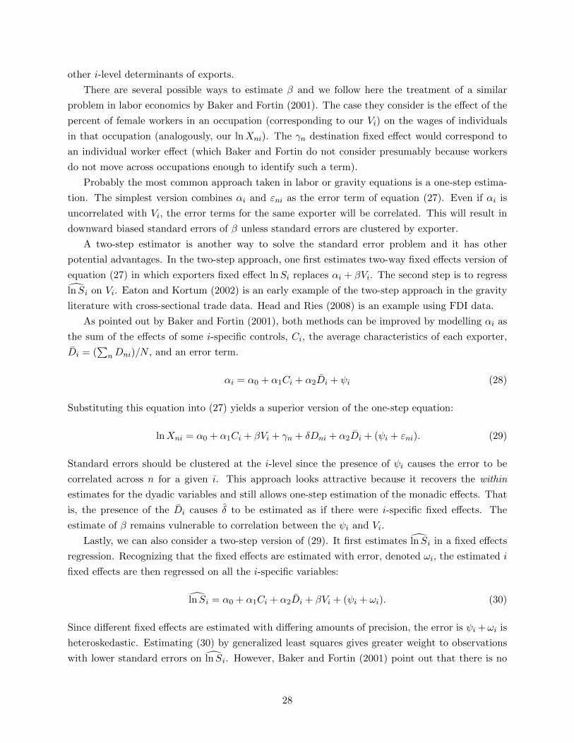
other i-level determinants of exports.
There are several possible ways to estimate β and we follow here the treatment of a similar
problem in labor economics by Baker and Fortin (2001). The case they consider is the effect of the
percent of female workers in an occupation (corresponding to our Vi) on the wages of individuals
in that occupation (analogously, our lnXni). The γn destination fixed effect would correspond to
an individual worker effect (which Baker and Fortin do not consider presumably because workers
do not move across occupations enough to identify such a term).
Probably the most common approach taken in labor or gravity equations is a one-step estima-
tion. The simplest version combines αi and εni as the error term of equation (27). Even if αi is
uncorrelated with Vi, the error terms for the same exporter will be correlated. This will result in
downward biased standard errors of β unless standard errors are clustered by exporter.
A two-step estimator is another way to solve the standard error problem and it has other
potential advantages. In the two-step approach, one first estimates two-way fixed effects version of
equation (27) in which exporters fixed effect lnSi replaces αi + βVi. The second step is to regress
lnSi on Vi. Eaton and Kortum (2002) is an early example of the two-step approach in the gravity
literature with cross-sectional trade data. Head and Ries (2008) is an example using FDI data.
As pointed out by Baker and Fortin (2001), both methods can be improved by modelling αi as
the sum of the effects of some i-specific controls, Ci, the average characteristics of each exporter,
Di = (∑
nDni)/N , and an error term.
αi = α0 + α1Ci + α2Di + ψi (28)
Substituting this equation into (27) yields a superior version of the one-step equation:
lnXni = α0 + α1Ci + βVi + γn + δDni + α2Di + (ψi + εni). (29)
Standard errors should be clustered at the i-level since the presence of ψi causes the error to be
correlated across n for a given i. This approach looks attractive because it recovers the within
estimates for the dyadic variables and still allows one-step estimation of the monadic effects. That
is, the presence of the Di causes δ to be estimated as if there were i-specific fixed effects. The
estimate of β remains vulnerable to correlation between the ψi and Vi.
Lastly, we can also consider a two-step version of (29). It first estimates lnSi in a fixed effects
regression. Recognizing that the fixed effects are estimated with error, denoted ωi, the estimated i
fixed effects are then regressed on all the i-specific variables:
lnSi = α0 + α1Ci + α2Di + βVi + (ψi + ωi). (30)
Since different fixed effects are estimated with differing amounts of precision, the error is ψi +ωi is
heteroskedastic. Estimating (30) by generalized least squares gives greater weight to observations
with lower standard errors on lnSi. However, Baker and Fortin (2001) point out that there is no
28
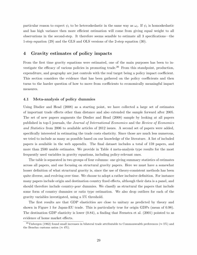
particular reason to expect ψi to be heteroskedastic in the same way as ωi. If ψi is homoskedastic
and has high variance then more efficient estimation will come from giving equal weight to all
observations in the second-step. It therefore seems sensible to estimate all 3 specifications—the
1-step equation (29) and the GLS and OLS versions of the 2-step equation (30).
4 Gravity estimates of policy impacts
From the first time gravity equations were estimated, one of the main purposes has been to in-
vestigate the efficacy of various policies in promoting trade.26 From this standpoint, production,
expenditure, and geography are just controls with the real target being a policy impact coefficient.
This section considers the evidence that has been gathered on the policy coefficients and then
turns to the harder question of how to move from coefficients to economically meaningful impact
measures.
4.1 Meta-analysis of policy dummies
Using Disdier and Head (2008) as a starting point, we have collected a large set of estimates
of important trade effects other than distance and also extended the sample forward after 2005.
The set of new papers augments the Disdier and Head (2008) sample by looking at all papers
published in top-5 journals, the Journal of International Economics and the Review of Economics
and Statistics from 2006 to available articles of 2012 issues. A second set of papers were added,
specifically interested in estimating the trade costs elasticity. Since those are much less numerous,
we tried to include as many as possible based on our knowledge of the literature. A list of included
papers is available in the web appendix. The final dataset includes a total of 159 papers, and
more than 2500 usable estimates. We provide in Table 4 meta-analysis type results for the most
frequently used variables in gravity equations, including policy-relevant ones.
The table is separated in two groups of four columns: one giving summary statistics of estimates
across all papers, and one focusing on structural gravity papers. Here we must have a somewhat
looser definition of what structural gravity is, since the use of theory-consistent methods has been
quite diverse, and evolving over time. We choose to adopt a rather inclusive definition. For instance
many papers include origin and destination country fixed effects, although their data is a panel, and
should therefore include country-year dummies. We classify as structural the papers that include
some form of country dummies or ratio type estimation. We also drop outliers for each of the
gravity variables investigated, using a 5% threshold.
The first results are that GDP elasticities are close to unitary as predicted by theory and
shown in Figure 1 for Japan-EU trade. This is particularly true for origin GDPs (mean of 0.98).
The destination GDP elasticity is lower (0.84), a finding that Feenstra et al. (2001) pointed to as
evidence of home market effects.
26Tinbergen (1962) found small increases in bilateral trade attributable to Commonwealth preferences (≈ 5%) andthe Benelux customs union (≈ 4%).
29
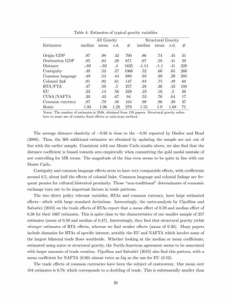
Table 4: Estimates of typical gravity variables
All Gravity Structural GravityEstimates: median mean s.d. # median mean s.d. #
Origin GDP .97 .98 .42 700 .86 .74 .45 31Destination GDP .85 .84 .28 671 .67 .58 .41 29Distance -.89 -.93 .4 1835 -1.14 -1.1 .41 328Contiguity .49 .53 .57 1066 .52 .66 .65 266Common language .49 .54 .44 680 .33 .39 .29 205Colonial link .91 .92 .61 147 .84 .75 .49 60RTA/FTA .47 .59 .5 257 .28 .36 .42 108EU .23 .14 .56 329 .19 .16 .5 26CUSA/NAFTA .39 .43 .67 94 .53 .76 .64 17Common currency .87 .79 .48 104 .98 .86 .39 37Home 1.93 1.96 1.28 279 1.55 1.9 1.68 71
Notes: The number of estimates is 2508, obtained from 159 papers. Structural gravity refershere to some use of country fixed effects or ratio-type method.
The average distance elasticity of −0.93 is close to the −0.91 reported by Disdier and Head
(2008). Thus, the 368 additional estimates we obtained by updating the sample are not out of
line with the earlier sample. Consistent with our Monte Carlo results above, we also find that the
distance coefficient is biased towards zero empirically when committing the gold medal mistake of
not controlling for MR terms. The magnitude of the bias even seems to be quite in line with our
Monte Carlo.
Contiguity and common language effects seem to have very comparable effects, with coefficients
around 0.5, about half the effects of colonial links. Common language and colonial linkage are fre-
quent proxies for cultural/historical proximity. Those “non-traditional” determinants of economic
exchange turn out to be important factors in trade patterns.
The two direct policy relevant variables, RTAs and common currency, have large estimated
effects—albeit with large standard deviations. Interestingly, the meta-analysis by Cipollina and
Salvatici (2010) on the trade effects of RTAs report that a mean effect of 0.59 and median effect of
0.38 for their 1867 estimates. This is quite close to the characteristics of our smaller sample of 257
estimates (mean of 0.59 and median of 0.47). Interestingly, they find that structural gravity yields
stronger estimates of RTA effects, whereas we find weaker effects (mean of 0.36). Many papers
include dummies for RTAs of specific interest, notably the EU and NAFTA which involve some of
the largest bilateral trade flows worldwide. Whether looking at the median or mean coefficients,
estimated using naive or structural gravity, the North-American agreement seems to be associated
with larger amounts of trade creation. Cipollina and Salvatici (2010) also find this pattern, with a
mean coefficient for NAFTA (0.90) almost twice as big as the one for EU (0.52).
The trade effects of common currencies have been the subject of controversy. Our mean over
104 estimates is 0.79, which corresponds to a doubling of trade. This is substantially smaller than
30
initial estimates by Rose (2000) who put the currency union coefficient at 1.21, implying more
than tripling trade. However, the meta-analysis average is substantially larger than the preferred
estimates of some recent work. Baldwin (2006), synthesizing a stream of papers focusing mainly on
the Euro, puts the currency effect at about 30%. Santos Silva and Tenreyro (2010) find virtually
no effects on trade for the Euro, after taking account the high level of trade integration of Eurozone
members even before they formed a common currency. Berthou and Fontagne (2012) use firm-level
exports by French firms and find a weakly significant 5% effect, coming mostly from average exports
by the most productive firms. Frankel (2010) finds a more optimistic 15% increase of trade that
takes about 5 years to take place, and then stabilizes.27
The numbers reported in Table 4 establish the typical findings but they should not be interpreted
as preferred estimates of the causal effects of the policy variables. This is because by and large they
fail to address the endogeneity related to many of the policy variables and especially to currency
unions and RTAs. There are many examples where the countries that sign a trade enhancing
agreement already trade a great deal together (NAFTA, EU). Since currency unions economize on
transaction costs of converting exchange, they will be greater when there are more transactions, that
is when countries trade a lot with each other. Cross-section or pooled panel estimates are therefore
not reliable—even if they have country or country-year fixed effects. The textbook solution would be
to find instrumental variables but we are not aware of any compelling instruments. Most variables
that plausibly cause currency unions or RTAs also “belong” in the trade equation on their own
(e.g. distance, colonial history). Lacking plausible IVs, the most promising approach is to include
country-pair fixed effects. This forces identification to come from the within dimension of the data.
Studies that introduce dyadic fixed effects often obtain dramatically different coefficient estimates
from the pooled OLS estimates.28 Another strategy is to use a natural experiment. In the final
part of the paper, Frankel (2010) uses the conversion of the French Franc to the euro in 1999 as an
exogenous shock hitting Western African countries that had the CFA Franc (linked to the French
Franc) as a currency. The switch to a common currency with members of the eurozone other
than France can reasonably be considered as exogenous for this group of African countries. The
trade creating effect seems stronger with this method (around 50%) than with the more classical
approach used in the first part of this paper. It also coincides with the switch to the euro, although
coefficients puzzlingly lose significance in the two last years of the sample (2005 and 2006).
27Differences might come from different sets of fixed effects, and also from different estimators. Baldwin andTaglioni (2007, table 4) turn the Eurozone coefficient from a significant positive 0.17 with OLS, to a significant -0.09with the appropriate set of country-year and country-pair fixed effects that account for MR terms, and identify inthe within dimension. Santos Silva and Tenreyro (2010) have similar identification strategy and results, with PPMLrather than a linear in logs estimator. Frankel (2010) regressions have a country pair fixed effect, but not the countryyear dummies that would control for MR terms.
28For instance, Baier and Bergstrand (2007) find that the RTA estimate is multiplied by more than two, whileGlick and Rose (2002) find that the common currency effect is divided by around the same factor. Head et al. (2010)also conduct a dyadic fixed effect specification. Compared to a naive specification, they find a rise in the effect ofGATT/WTO (which is also the case in Rose (2004)), and confirm the fall in common currency effects. On RTA theyfind that the coefficient is halved, in contrast to the results of Baier and Bergstrand (2007).
31
4.2 The elasticity of trade with respect to trade costs
Arkolakis et al. (2012b) show that a gravity equation is all that is needed to calculate welfare
gains from trade. Indeed, of the two sufficient statistics required when their macro restrictions
hold, one is directly observable (the import ratio), and the other, the trade cost elasticity of trade,
can be estimated using a gravity equation for bilateral trade. While relatively few gravity papers
estimate trade cost elasticities, we have identified 32 papers that do so, and we summarize their
results in Table 5. We will refer to those as “gravity-based” estimates. They involve regressing
bilateral trade on measures of bilateral trade costs or on exporter “competitiveness” such as wages
or productivity.29 About three quarters of our estimates of ε are of the first type, and come from
regressions along the lines of
lnXni = lnSi + lnMn + ε ln τni. (31)
In many cases, equation (31) is estimated at the industry level. This explains in part the very large
variance observed across estimates in the literature, reported in Table 5 below.30 Most specifications
measure ln τni as the log of one plus the ad valorem bilateral tariff rate. In some cases the ad valorem
freight rates are used instead of or in addition to tariff rates (Hummels (1999) in particular).
We define the gravity-based method broadly enough to encompass estimates derived from re-
gressing bilateral trade on proxies for exporter competitiveness such as wages, exchange rates, and
prices. The precise implementation of the competitiveness-based estimate can take two forms: 1)
estimate the exporter in a first stage and regress it on wages in a second stage, 2) directly estimate
the bilateral equation using the determinants of Si, including wages. Eaton and Kortum (2002) is
an example of the first approach. They regress exporter fixed effects (derived from a transformed
bilateral trade variable) on proxies for technology (R&D expenditures, average years of education)
and wages. Instrumenting for wages, they obtain an elasticity of −3.6. As with the trade cost
methods, this approach is actually more general than the precise model used by Eaton and Kortum
(2002). Indeed, when looking at Table 1, we see that the wage in the origin country exhibits an
elasticity that is the same or closely related to the elasticity with respect to bilateral trade costs in
most foundations of gravity. In Eaton and Kortum (2002), the wage elasticity is −βθ whereas the
trade elasticity is −θ. Thus, if we know β (the share of wages in the cost function in their model),
the effect of wage variation on estimated lnSi is an alternative source of identification for the same
key parameter.31 The second approach is chosen by Costinot et al. (2012), who estimate a trade
29In addition to the gravity-based estimates included in our meta-analysis, there are two other influential ap-proaches. One method, devised by Feenstra (1994) and applied more broadly by Broda and Weinstein (2006), is toestimate the “Armington” elasticity, σ, using GMM identification via heteroskedasticity. Then 1−σ could be used asthe estimate of ε. A second method originated by Eaton and Kortum (2002) and refined by Simonovska and Waugh(2011), estimates ε by relating trade variation to price gaps.
30Taking into account this heterogeneity has been shown recently to be particularly important for the estimation ofwelfare gains from trade, which are larger when ε varies across sectors (see Ossa (2012) and Costinot and Rodriguez-Clare (2013) for expositions and estimations of the aggregation bias in welfare gains calculations).
31Since wages are likely to be simultaneously determined with trade patterns, it seems important to instrument forwages, and indeed, the estimated parameter seems to be systematically larger (in absolute value) when instrumenting.
32
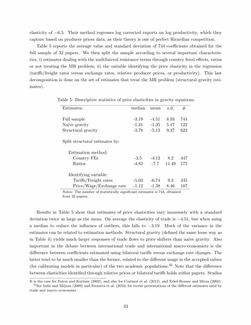
elasticity of −6.5. Their method regresses log corrected exports on log productivity, which they
capture based on producer prices data, as their theory is one of perfect Ricardian competition.
Table 5 reports the average value and standard deviation of 744 coefficients obtained for the
full sample of 32 papers. We then split the sample according to several important characteris-
tics, i) estimates dealing with the multilateral resistance terms through country fixed effects, ratios
or not treating the MR problem; ii) the variable identifying the price elasticity in the regression
(tariffs/freight rates versus exchange rates, relative producer prices, or productivity). This last
decomposition is done on the set of estimates that treat the MR problem (structural gravity esti-
mates).
Table 5: Descriptive statistics of price elasticities in gravity equations
Estimates: median mean s.d. #
Full sample -3.19 -4.51 8.93 744Naive gravity -1.31 -1.35 5.17 122Structural gravity -3.78 -5.13 9.37 622
Split structural estimates by:
Estimation method:Country FEs -3.5 -4.12 8.2 447Ratios -4.82 -7.7 11.49 175
Identifying variable:Tariffs/Freight rates -5.03 -6.74 9.3 435Price/Wage/Exchange rate -1.12 -1.38 8.46 187
Notes: The number of statistically significant estimates is 744, obtainedfrom 32 papers.
Results in Table 5 show that estimates of price elasticities vary immensely with a standard
deviation twice as large as the mean. On average the elasticity of trade is −4.51, but when using
a median to reduce the influence of outliers, this falls to −3.19. Much of the variance in the
estimates can be related to estimation methods: Structural gravity (defined the same loose way as
in Table 4) yields much larger responses of trade flows to price shifters than naive gravity. Also
important in the debate between international trade and international macro-economists is the
difference between coefficients estimated using bilateral tariffs versus exchange rate changes. The
latter tend to be much smaller than the former, related to the different usage in the accepted values
(for calibrating models in particular) of the two academic populations.32 Note that the difference
between elasticities identified through relative prices or bilateral tariffs holds within papers. Studies
It is the case for Eaton and Kortum (2002), and also for Costinot et al. (2012), and Erkel-Rousse and Mirza (2002).32See Imbs and Mejean (2009) and Feenstra et al. (2010) for recent presentations of the different estimates used by
trade and macro economists.
33
such as De Sousa et al. (2012) and Fitzgerald and Haller (2012) which estimate the effects of
exchange rates and tariffs in the same regressions find comparable differences to ones seen in
Table 5. Overall, our preferred estimate for ε is −5.03, the median coefficient obtained using tariff
variation, while controlling for multilateral resistance terms.
Armed with this estimate of the trade elasticity, we can do a simple calculation to determine
if estimated RTA effects in Table 4 are reasonable. Let ρ be the estimated coefficient on the
RTA dummy variable. Since it measures the reduction in trade costs achieved by the RTA, ρ =
ε(ln τMFNni − ln τRTA
ni ), where τMFNni is the “most-favored-nation” trade cost factor that n would apply
to imports from i were they not in a free trade agreement. Denote as t the MFN tariffs that must be
removed in the RTA (as per GATT article 24) and let κ capture the ad-valorem tariff-equivalent of
all trade barriers that remain in force after the implementation of the RTA. Then τMFNni = 1 +κ+ t
and τRTAni = 1 + κ. After some algebra, we obtain t = (1 + κ)[exp(ρ/ε) − 1]. Martin et al. (2012)
estimate ρ = 0.26, implicitly assume κ = 0, and set ε = 4 to calculate t = exp(0.26/4) = 6.7%.
With our median structural gravity estimate of ρ = 0.28 and tariff-based ε = −5.03, assuming κ = 0
implies t = 5.7%. The problem with this assumption is that “home” (trade with self) coefficients
are estimated at 1.55. This implies κ = exp(1.55/5.03)− 1 = 36%. Substituting this value back in
yields t = 7.8%. This is considerably higher than the current 3.83% weighted world MFN tariff but
lower than the 2000 world simple average MFN tariff of 12.8% (both reported by World Bank WDI
database). Thus, our results on border effects, RTA impacts, and trade elasticities are mutually
consistent with the proposition that the main channel through which RTAs liberalize trade is the
elimination of MFN tariffs. The more general point is that to be in line with actual tariffs, the
trade elasticity should be somewhat over ten times the RTA coefficient; our meta-analysis suggests
this is indeed the case.
4.3 Partial vs general equilibrium impacts on trade
The consideration of price index and multilateral resistance terms is not only important from
the point of view of estimating the correct β for each of the variables that comprise the trade cost
determinants. A second point that Anderson and van Wincoop (2003) emphasize is that the indexes
change when trade costs change. Thus, merely exponentiating the coefficients on dummy variables
(which we will call the Partial Trade Impact, PTI) may not give a reliable estimate of the full impact
on trade. Indeed, one of the points emphasized by Anderson and van Wincoop (2003) is that taking
into account price index changes leads to substantially smaller trade impacts of borders. The trade
impact holding production and expenditure constant but adjusting Φn and Ωi via the contraction
mapping does not have an obvious name. It should not really be thought of as a general equilibrium
impact because it holds GDP constant and the GDPs depend on factor prices. Anderson (2011)
emphasizes the modular nature of the structural gravity model: the determination of output and
expenditures occurs in a different module from the allocation of bilateral flows. Hence, we will
label the trade impact that observes this feature of the model the Modular Trade Impact (MTI).
We reserve the title of General Equilibrium Trade Impact (GETI) for the case where wages (and
34

therefore GDPs) also adjust to trade cost changes.
Suppose that Bni is one of the bilateral variables determining τni. Further suppose that lnφni
is linear in Bni with coefficient β. We want to see the impact on trade of changing Bni to B′ni.
Holding the multilateral terms constant the ratio of new to original trade is just the ratio of new
to original trade freeness. Thus the partial trade impact is given by
PTIni = φni = φ′ni/φni = exp[β(B′ni −Bni)]. (32)
Note that PTIni = 0 for any country pair that does not change bilateral linkages, i.e. B′ni =
Bni. Thus, the PTI omits third-country effects, which are to be expected because the multilateral
resistance terms change whenever other countries change their trade costs.
For any trade equation fitting into structural gravity, the ratio of new bilateral trade, X ′ni, to
original trade taking MR changes into account (but leaving incomes unchanged) is obtained from
equation (2) as
MTIni =X ′niXni
= exp[β(B′ni −Bni)]︸ ︷︷ ︸PTI
× Ωi
Ω′i
Φn
Φ′n︸ ︷︷ ︸MR adjustment
(33)
The procedure to implement is therefore to retrieve lnφni, including coefficient β for Bni either
using estimates from the literature or estimating φni through an implementation of equation (22).
Then, using φni, Yi and Xn in equation (3), a contraction mapping gives us Φn and Ωi. The third
step is to do a counterfactual change to Bni (for instance, turn off all RTAs), which results in a
new freeness of trade index φ′ni. Re-running the contraction mapping provides us with Φ′n and Ω′i.
We have all the needed elements to calculate X ′ni/Xni. Contrary to the PTI approach, a change in
a variable specific to a pair of country using this approach will provide counterfactual changes in
trade flows for all country pairs.
A growing number of papers, following the initial motivation for structural estimation, do
counterfactuals using MTI (although the terminologies vary). Glick and Taylor (2010) is an example
where MTI is used to estimate the costs of military conflicts. Anderson and Yotov (2010a) apply
this method to assess the impact of an agreement on trade between Canadian provinces that took
place in 1995.
An important issue with the MTI is that while (33) does account for changes in MR terms
(Φn and Ωi), it assumes constant expenditure (Xn) and output (Yi) for all countries, which raises a
question of interpretation. Recall that Si = Yi/Ωi. Holding Yi constant, it must be that S′i = Yi/Ω′i.
The conceptual problem is that Si in many models summarized in Table 1 depends on wages and
exogenous parameters such as quality, A, or technology, T , of all products manufactured in i.
Changes in trade costs are not permitted to change wages since that would affect Yi, but it is
peculiar to allow trade costs to change deep parameters.
A second issue is that MTI may omit potentially important effects. For instance, if the thought
experiment is the removal of trade costs with a major partner, it is very unlikely that such a
drastic change in the trade cost matrix, and therefore in predicted trade flows, would leave incomes
35
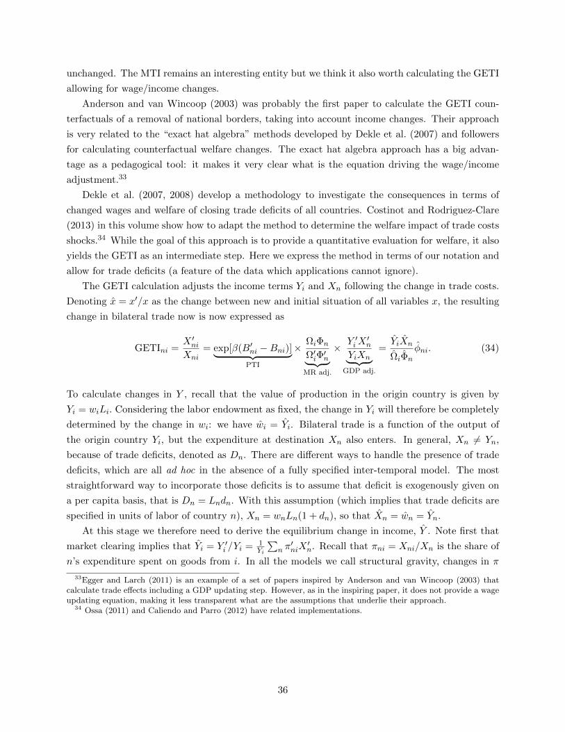
unchanged. The MTI remains an interesting entity but we think it also worth calculating the GETI
allowing for wage/income changes.
Anderson and van Wincoop (2003) was probably the first paper to calculate the GETI coun-
terfactuals of a removal of national borders, taking into account income changes. Their approach
is very related to the “exact hat algebra” methods developed by Dekle et al. (2007) and followers
for calculating counterfactual welfare changes. The exact hat algebra approach has a big advan-
tage as a pedagogical tool: it makes it very clear what is the equation driving the wage/income
adjustment.33
Dekle et al. (2007, 2008) develop a methodology to investigate the consequences in terms of
changed wages and welfare of closing trade deficits of all countries. Costinot and Rodriguez-Clare
(2013) in this volume show how to adapt the method to determine the welfare impact of trade costs
shocks.34 While the goal of this approach is to provide a quantitative evaluation for welfare, it also
yields the GETI as an intermediate step. Here we express the method in terms of our notation and
allow for trade deficits (a feature of the data which applications cannot ignore).
The GETI calculation adjusts the income terms Yi and Xn following the change in trade costs.
Denoting x = x′/x as the change between new and initial situation of all variables x, the resulting
change in bilateral trade now is now expressed as
GETIni =X ′niXni
= exp[β(B′ni −Bni)]︸ ︷︷ ︸PTI
× ΩiΦn
Ω′iΦ′n︸ ︷︷ ︸
MR adj.
× Y ′iX′n
YiXn︸ ︷︷ ︸GDP adj.
=YiXn
ΩiΦn
φni. (34)
To calculate changes in Y , recall that the value of production in the origin country is given by
Yi = wiLi. Considering the labor endowment as fixed, the change in Yi will therefore be completely
determined by the change in wi: we have wi = Yi. Bilateral trade is a function of the output of
the origin country Yi, but the expenditure at destination Xn also enters. In general, Xn 6= Yn,
because of trade deficits, denoted as Dn. There are different ways to handle the presence of trade
deficits, which are all ad hoc in the absence of a fully specified inter-temporal model. The most
straightforward way to incorporate those deficits is to assume that deficit is exogenously given on
a per capita basis, that is Dn = Lndn. With this assumption (which implies that trade deficits are
specified in units of labor of country n), Xn = wnLn(1 + dn), so that Xn = wn = Yn.
At this stage we therefore need to derive the equilibrium change in income, Y . Note first that
market clearing implies that Yi = Y ′i /Yi = 1Yi
∑n π′niX
′n. Recall that πni = Xni/Xn is the share of
n’s expenditure spent on goods from i. In all the models we call structural gravity, changes in π
33Egger and Larch (2011) is an example of a set of papers inspired by Anderson and van Wincoop (2003) thatcalculate trade effects including a GDP updating step. However, as in the inspiring paper, it does not provide a wageupdating equation, making it less transparent what are the assumptions that underlie their approach.
34 Ossa (2011) and Caliendo and Parro (2012) have related implementations.
36
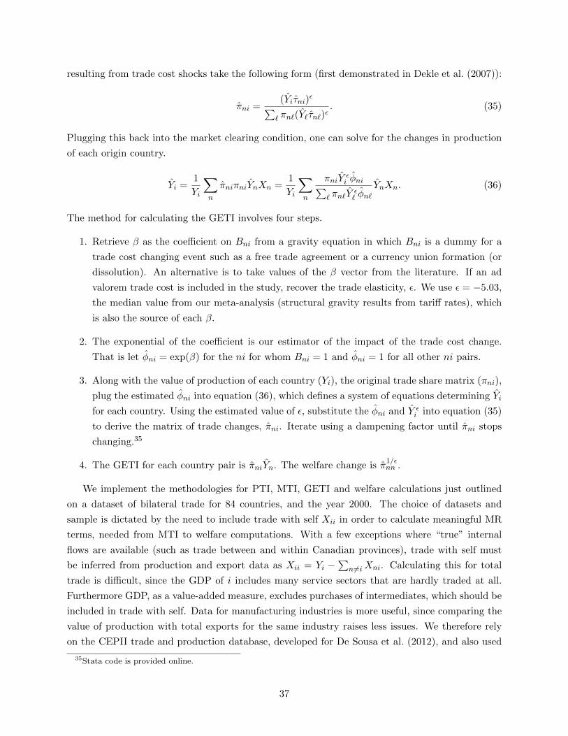
resulting from trade cost shocks take the following form (first demonstrated in Dekle et al. (2007)):
πni =(Yiτni)
ε∑` πn`(Y`τn`)
ε. (35)
Plugging this back into the market clearing condition, one can solve for the changes in production
of each origin country.
Yi =1
Yi
∑n
πniπniYnXn =1
Yi
∑n
πniYεi φni∑
` πn`Yε` φn`
YnXn. (36)
The method for calculating the GETI involves four steps.
1. Retrieve β as the coefficient on Bni from a gravity equation in which Bni is a dummy for a
trade cost changing event such as a free trade agreement or a currency union formation (or
dissolution). An alternative is to take values of the β vector from the literature. If an ad
valorem trade cost is included in the study, recover the trade elasticity, ε. We use ε = −5.03,
the median value from our meta-analysis (structural gravity results from tariff rates), which
is also the source of each β.
2. The exponential of the coefficient is our estimator of the impact of the trade cost change.
That is let φni = exp(β) for the ni for whom Bni = 1 and φni = 1 for all other ni pairs.
3. Along with the value of production of each country (Yi), the original trade share matrix (πni),
plug the estimated φni into equation (36), which defines a system of equations determining Yi
for each country. Using the estimated value of ε, substitute the φni and Y εi into equation (35)
to derive the matrix of trade changes, πni. Iterate using a dampening factor until πni stops
changing.35
4. The GETI for each country pair is πniYn. The welfare change is π1/εnn .
We implement the methodologies for PTI, MTI, GETI and welfare calculations just outlined
on a dataset of bilateral trade for 84 countries, and the year 2000. The choice of datasets and
sample is dictated by the need to include trade with self Xii in order to calculate meaningful MR
terms, needed from MTI to welfare computations. With a few exceptions where “true” internal
flows are available (such as trade between and within Canadian provinces), trade with self must
be inferred from production and export data as Xii = Yi −∑
n 6=iXni. Calculating this for total
trade is difficult, since the GDP of i includes many service sectors that are hardly traded at all.
Furthermore GDP, as a value-added measure, excludes purchases of intermediates, which should be
included in trade with self. Data for manufacturing industries is more useful, since comparing the
value of production with total exports for the same industry raises less issues. We therefore rely
on the CEPII trade and production database, developed for De Sousa et al. (2012), and also used
35Stata code is provided online.
37
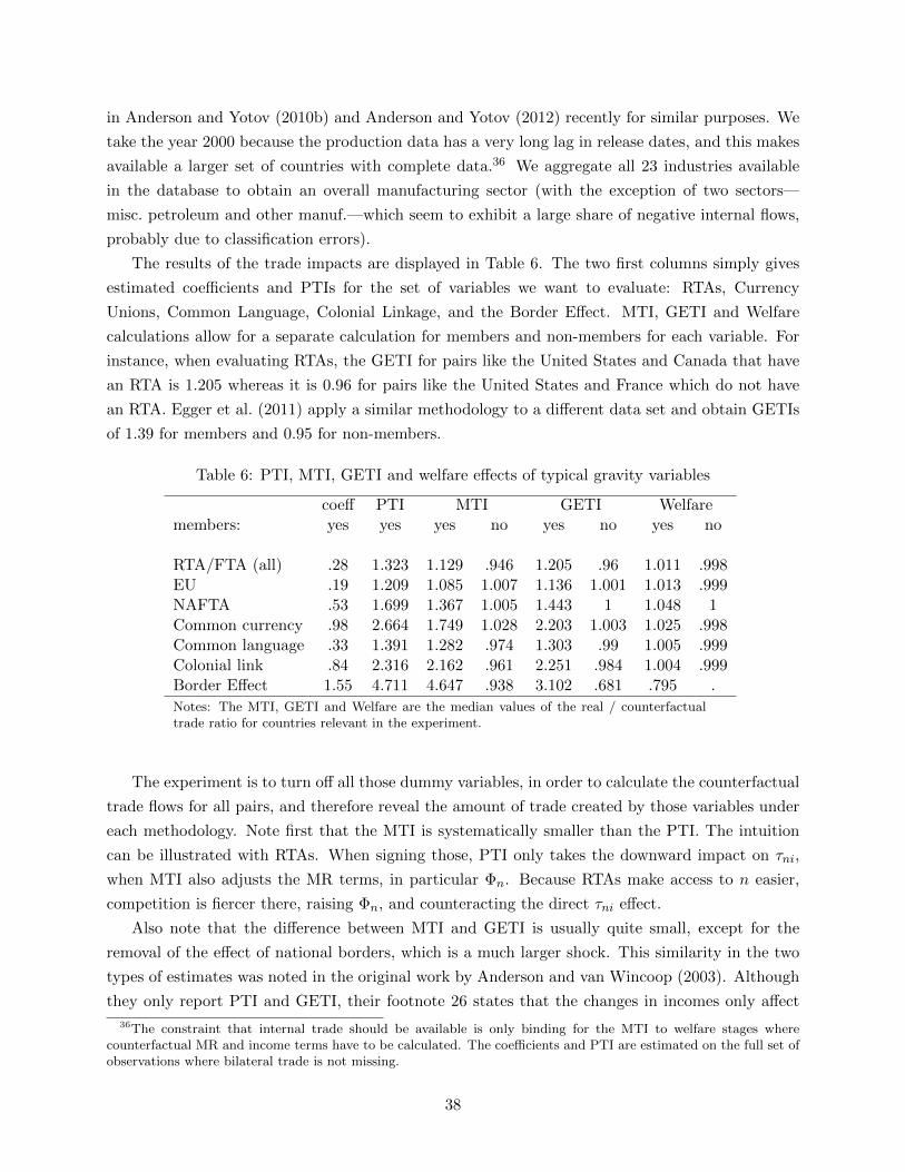
in Anderson and Yotov (2010b) and Anderson and Yotov (2012) recently for similar purposes. We
take the year 2000 because the production data has a very long lag in release dates, and this makes
available a larger set of countries with complete data.36 We aggregate all 23 industries available
in the database to obtain an overall manufacturing sector (with the exception of two sectors—
misc. petroleum and other manuf.—which seem to exhibit a large share of negative internal flows,
probably due to classification errors).
The results of the trade impacts are displayed in Table 6. The two first columns simply gives
estimated coefficients and PTIs for the set of variables we want to evaluate: RTAs, Currency
Unions, Common Language, Colonial Linkage, and the Border Effect. MTI, GETI and Welfare
calculations allow for a separate calculation for members and non-members for each variable. For
instance, when evaluating RTAs, the GETI for pairs like the United States and Canada that have
an RTA is 1.205 whereas it is 0.96 for pairs like the United States and France which do not have
an RTA. Egger et al. (2011) apply a similar methodology to a different data set and obtain GETIs
of 1.39 for members and 0.95 for non-members.
Table 6: PTI, MTI, GETI and welfare effects of typical gravity variables
coeff PTI MTI GETI Welfaremembers: yes yes yes no yes no yes no
RTA/FTA (all) .28 1.323 1.129 .946 1.205 .96 1.011 .998EU .19 1.209 1.085 1.007 1.136 1.001 1.013 .999NAFTA .53 1.699 1.367 1.005 1.443 1 1.048 1Common currency .98 2.664 1.749 1.028 2.203 1.003 1.025 .998Common language .33 1.391 1.282 .974 1.303 .99 1.005 .999Colonial link .84 2.316 2.162 .961 2.251 .984 1.004 .999Border Effect 1.55 4.711 4.647 .938 3.102 .681 .795 .
Notes: The MTI, GETI and Welfare are the median values of the real / counterfactualtrade ratio for countries relevant in the experiment.
The experiment is to turn off all those dummy variables, in order to calculate the counterfactual
trade flows for all pairs, and therefore reveal the amount of trade created by those variables under
each methodology. Note first that the MTI is systematically smaller than the PTI. The intuition
can be illustrated with RTAs. When signing those, PTI only takes the downward impact on τni,
when MTI also adjusts the MR terms, in particular Φn. Because RTAs make access to n easier,
competition is fiercer there, raising Φn, and counteracting the direct τni effect.
Also note that the difference between MTI and GETI is usually quite small, except for the
removal of the effect of national borders, which is a much larger shock. This similarity in the two
types of estimates was noted in the original work by Anderson and van Wincoop (2003). Although
they only report PTI and GETI, their footnote 26 states that the changes in incomes only affect
36The constraint that internal trade should be available is only binding for the MTI to welfare stages wherecounterfactual MR and income terms have to be calculated. The coefficients and PTI are estimated on the full set ofobservations where bilateral trade is not missing.
38
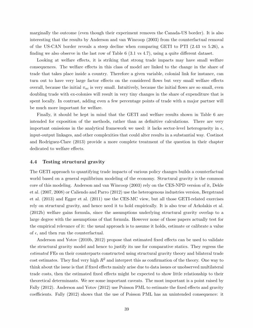
marginally the outcome (even though their experiment removes the Canada-US border). It is also
interesting that the results by Anderson and van Wincoop (2003) from the counterfactual removal
of the US-CAN border reveals a steep decline when comparing GETI to PTI (2.43 vs 5.26), a
finding we also observe in the last row of Table 6 (3.1 vs 4.7), using a quite different dataset.
Looking at welfare effects, it is striking that strong trade impacts may have small welfare
consequences. The welfare effects in this class of model are linked to the change in the share of
trade that takes place inside a country. Therefore a given variable, colonial link for instance, can
turn out to have very large factor effects on the considered flows but very small welfare effects
overall, because the initial πni is very small. Intuitively, because the initial flows are so small, even
doubling trade with ex-colonies will result in very tiny changes in the share of expenditure that is
spent locally. In contrast, adding even a few percentage points of trade with a major partner will
be much more important for welfare.
Finally, it should be kept in mind that the GETI and welfare results shown in Table 6 are
intended for exposition of the methods, rather than as definitive calculations. There are very
important omissions in the analytical framework we used: it lacks sector-level heterogeneity in ε,
input-output linkages, and other complexities that could alter results in a substantial way. Costinot
and Rodriguez-Clare (2013) provide a more complete treatment of the question in their chapter
dedicated to welfare effects.
4.4 Testing structural gravity
The GETI approach to quantifying trade impacts of various policy changes builds a counterfactual
world based on a general equilibrium modeling of the economy. Structural gravity is the common
core of this modeling. Anderson and van Wincoop (2003) rely on the CES-NPD version of it, Dekle
et al. (2007, 2008) or Caliendo and Parro (2012) use the heterogenous industries version, Bergstrand
et al. (2013) and Egger et al. (2011) use the CES-MC view, but all those GETI-related exercises
rely on structural gravity, and hence need it to hold empirically. It is also true of Arkolakis et al.
(2012b) welfare gains formula, since the assumptions underlying structural gravity overlap to a
large degree with the assumptions of that formula. However none of those papers actually test for
the empirical relevance of it: the usual approach is to assume it holds, estimate or calibrate a value
of ε, and then run the counterfactual.
Anderson and Yotov (2010b, 2012) propose that estimated fixed effects can be used to validate
the structural gravity model and hence to justify its use for comparative statics. They regress the
estimated FEs on their counterparts constructed using structural gravity theory and bilateral trade
cost estimates. They find very high R2 and interpret this as confirmation of the theory. One way to
think about the issue is that if fixed effects mainly arise due to data issues or unobserved multilateral
trade costs, then the estimated fixed effects might be expected to show little relationship to their
theoretical determinants. We see some important caveats. The most important is a point raised by
Fally (2012). Anderson and Yotov (2012) use Poisson PML to estimate the fixed effects and gravity
coefficients. Fally (2012) shows that the use of Poisson PML has an unintended consequence: it
39
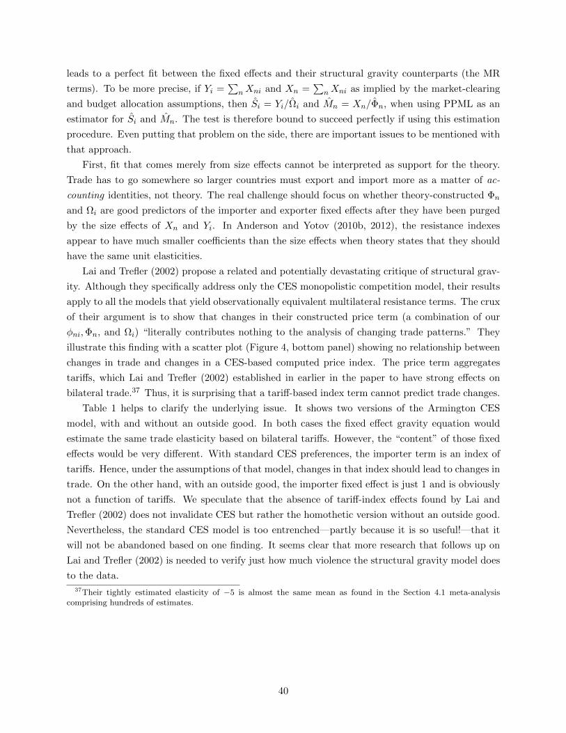
leads to a perfect fit between the fixed effects and their structural gravity counterparts (the MR
terms). To be more precise, if Yi =∑
nXni and Xn =∑
nXni as implied by the market-clearing
and budget allocation assumptions, then Si = Yi/Ωi and Mn = Xn/Φn, when using PPML as an
estimator for Si and Mn. The test is therefore bound to succeed perfectly if using this estimation
procedure. Even putting that problem on the side, there are important issues to be mentioned with
that approach.
First, fit that comes merely from size effects cannot be interpreted as support for the theory.
Trade has to go somewhere so larger countries must export and import more as a matter of ac-
counting identities, not theory. The real challenge should focus on whether theory-constructed Φn
and Ωi are good predictors of the importer and exporter fixed effects after they have been purged
by the size effects of Xn and Yi. In Anderson and Yotov (2010b, 2012), the resistance indexes
appear to have much smaller coefficients than the size effects when theory states that they should
have the same unit elasticities.
Lai and Trefler (2002) propose a related and potentially devastating critique of structural grav-
ity. Although they specifically address only the CES monopolistic competition model, their results
apply to all the models that yield observationally equivalent multilateral resistance terms. The crux
of their argument is to show that changes in their constructed price term (a combination of our
φni,Φn, and Ωi) “literally contributes nothing to the analysis of changing trade patterns.” They
illustrate this finding with a scatter plot (Figure 4, bottom panel) showing no relationship between
changes in trade and changes in a CES-based computed price index. The price term aggregates
tariffs, which Lai and Trefler (2002) established in earlier in the paper to have strong effects on
bilateral trade.37 Thus, it is surprising that a tariff-based index term cannot predict trade changes.
Table 1 helps to clarify the underlying issue. It shows two versions of the Armington CES
model, with and without an outside good. In both cases the fixed effect gravity equation would
estimate the same trade elasticity based on bilateral tariffs. However, the “content” of those fixed
effects would be very different. With standard CES preferences, the importer term is an index of
tariffs. Hence, under the assumptions of that model, changes in that index should lead to changes in
trade. On the other hand, with an outside good, the importer fixed effect is just 1 and is obviously
not a function of tariffs. We speculate that the absence of tariff-index effects found by Lai and
Trefler (2002) does not invalidate CES but rather the homothetic version without an outside good.
Nevertheless, the standard CES model is too entrenched—partly because it is so useful!—that it
will not be abandoned based on one finding. It seems clear that more research that follows up on
Lai and Trefler (2002) is needed to verify just how much violence the structural gravity model does
to the data.
37Their tightly estimated elasticity of −5 is almost the same mean as found in the Section 4.1 meta-analysiscomprising hundreds of estimates.
40
5 Frontiers of gravity research
This section investigates three areas of ongoing research. The first issue is how to appropriately
model the error term in the gravity equation, in particular considering the problem of heteroskedas-
ticity in multiplicative models. The second topic is the appropriate estimation response to large
numbers of zero trade flows, a phenomena at odds with a model in which predicted trade is a
multiple of strictly positive numbers. The last item covers the rising use of firm-level trade data
with its associated set of new issues regarding estimation and interpretation.
5.1 Gravity’s errors
Part of the original attraction of the gravity equation—and of other multiplicative models such as
the Cobb-Douglas production function—is that after taking logs they can be estimated with OLS.
Santos Silva and Tenreyro (2006) (hereafter SST) brought to the attention of the field that this
seemingly innocuous approach involves taking a much stronger stance on the functional form of the
error than we do when estimating truly linear models with OLS.
SST frame the problem in terms of heteroskedasticity but this begs the question of which error
is not homoskedastic. There are two ways of expressing the error in a gravity equation. Suppose
that the exporter and importer fixed effects as well as all determinants of φni have been combined
into a k-length vector zni and that the coefficients on these variables are vector ζ. The conventional
way to express the error is as the difference between data and prediction: εni ≡ Xni − exp(z′niζ).
The second way to express the error is as a ratio of data to prediction: ηni ≡ Xni/ exp(z′niζ).
After taking logs, the linear regression error term is given by lnXni−z′niζ = ln ηni. In standard
OLS regressions, heteroskedasticity of ln ηni is a minor concern. The grave concern is whether ln ηni
is independent from the zni. SST point out that if the variance of η depends on zni then the log
transformation will prevent ln ηni from having a zero conditional expectation and will therefore
lead to inconsistent coefficient estimates in linear (in logs) regression.
Should we then try to minimize the sum of the squared residuals, ε2ni, using non-linear least
squares? A homoskedastic additive error is an unappealing assumption. It defies common sense to
think that deviations of true trade from predicted trade would be of the same order of magnitude for
the US and Aruba. Moreover, SST find that NLLS performs very badly in Monte Carlo simulations.
SST argue that Poisson pseudo-maximum likelihood (PML) is an attractive alternative to linear-
in-logs OLS for multiplicative models like the gravity equation. Poisson is not the only PML that
could be applied to gravity equations and SST also consider Gamma PML. To understand what
each estimator is doing it is useful to compare their first order conditions side by side.
Actual exports are given by Xni = exp(z′niζ)ηni, where η is a multiplicative error term. Using∑to represent summation over all ni dyads, the moment conditions for the Poisson PML, OLS,
41
and Gamma PML are∑zni · (Xni − Xni) = 0︸ ︷︷ ︸
Poisson
,∑
zni · (lnXni − ln Xni) = 0︸ ︷︷ ︸OLS
,∑
zni · (Xni/Xni − 1) = 0︸ ︷︷ ︸Gamma
, (37)
where Xni ≡ exp(z′niζ) denotes the prediction forXni conditional on the observables. The first set of
first order conditions are the ones used for Poisson “true” MLE on count data. Comparing with the
OLS first order conditions we see that the Poisson involves level deviations of Xni from its expected
value whereas the OLS involves log deviations.38 The term in parentheses in the Gamma PML
FOC is just the percent deviation of actual trade from predicted trade. Since percent deviations are
approximately equal to log deviations, the Gamma PML pursues an objective that is very similar
to that of OLS shown in equation (37). A useful feature of the two PML is that FOC permit the
inclusion of zeros, unlike the linear-in-logs form. However, we delay treatment of the zero issue to
the following section so as to focus on the role of assumptions about the error term.
Both the Poisson and Gamma PML deliver consistent ζ estimates regardless of the distribution
of ηni so long as E[Xni | zni] = exp(z′niζ). The question of which one is more efficient depends on
how the variance of Xni relates to its expected value. Consider the following (fairly) general case:
Var[Xni | zni] = hE[Xni | zni]λ (38)
If λ = 1, a case we will call the Constant Variance to Mean Ratio (CVMR) assumption, then Poisson
PML is efficient. The CVMR assumption is a generalization of the Poisson variance assumption
in which h = λ = 1. The Gamma PML is the efficient PML if λ = 2, that is if the standard
deviation is proportional to the mean. We will therefore refer to a DGP that satisfies λ = 2 as one
that adheres to the Constant Coefficient of Variation (CCV) assumption. As the log-normal has
a CCV, this provides the intuition for why the Gamma PML estimates tend to be similar to the
OLS (on logs), since the latter is the MLE under the assumption of homoskedastic log-normality
(which we abbreviate as log-normality). Given that both Poisson and Gamma PML are consistent
under the same conditional expectation assumption, their estimates, ζ, should be approximately
the same if the sample is large enough. Their estimates will only converge on the OLS estimates
under log-normality of ηni.
Poisson and Gamma PML remain consistent (and efficient for the corresponding cases for λ)
even if h > 1, i.e. what is called “over-dispersion.” Thus, the finding that variance exceeds the mean
does not justify use of estimators such as the negative binomial, suggested by De Benedictis and
Taglioni (2011). This estimator is alluring because it has Poisson as a special case but estimates
what appears to be more general variance function with a parameter estimating the amount of
over-dispersion. We urge researchers to resist the siren song of the Negative Binomial. The most
important reason, pointed out by Boulhol and Bosquet (2012), is that Negative Binomial PML
38Wooldridge (2010, p. 741) provides further detail on the robustness and efficiency properties of Poisson PML.SST have provided responses to a variety of potential concerns about the Poisson PML estimator on their “log ofgravity” page.
42
estimates depend on the units of measurement for the dependent variable. The web appendix uses
actual data to show that measuring trade in thousands of dollars instead of billions not only leads
to large changes in the magnitudes of estimated elasticities, it even reverses the signs on some of
the indicator variables.39
Here we conduct Monte Carlo simulations that re-express some key insights derived from SST.
We illustrate attractive robustness features of PML estimators. For each repetition of the simulation
we also estimate a test statistic proposed by Manning and Mullahy (2001) to diagnose the error
term. This MaMu test—referred to by SST as a “Park-type” test—takes the log of equation (38)
and replaces the variance and expected value terms with their sample counterparts to obtain
ln ε2ni = constant + λ ln Xni, (39)
where ε = Xni − exp(z′niζ) and ln Xni = z′niζ. Equation (39) is estimated using OLS.
In order to focus on issues related to the distribution of the error term, the DGP does not
contain i, n, and ni-level components. Rather, as with the Monte Carlos of SST, it is a single-
dimensional cross-section. Also following SST, we include a continuous trade determinant, denoted
Dist for distance and assumed to be log-normal, as well as a binary variable, called RTA. The
results for the binary variable did not offer additional insights but they are available to interested
readers by running the program, which is available in the web appendix.
Figure 3 displays results for four versions of the following data generating process (where ui
denotes a standard normal pseudo-random term):
Xi = exp[θi ln Disti + 0.5RTAi + σi × ui].
Versions (a) and (b) have the usual distance elasticity (θi = −1) and differ regarding the assumed
error term. Cases (a) considers log-normal errors with a constant variance parameter σ = 2.
Case (b) departs from lognormal η by assuming a constant mean-variance ratio (CVMR), i.e.
heteroskedasticity a la Poisson. The σi is set to satisfy Var[Xi | RTAi,Disti] = h×exp[−1 ln Disti+
0.5RTAi]. Case (c) reverts to log-normal errors with σ = 2 but introduces a mis-specification. True
θi = −0.5 for Disti < Dist (where we set Dist equal to the median distance) and θi = −1.5 for
Disti ≥ Dist. Case (d) uses the same break in the distance elasticity but follows case (b) in using
as CVMR error. The regressions in (c) and (d) are mis-specified because they estimate a constant
distance elasticity.
The two left panels of Figure 3 consider the error term structure that is most favourable to OLS
and Gamma, that of log-normality with a σ parameter that is constant across all observations.
The key result in panel (a) is that Poisson PML underestimates the (absolute) magnitude of the
distance effect (and, while not shown, the RTA effect), but that estimates converge on the true
value as the sample size rises. The bias exhibited by Poisson PML in panel (a) is increasing in the
39Other drawbacks of the negative binomial include (a) as pointed out in Wooldridge (2010, p. 738), the one-stepform of Stata’s negbin command lacks the robustness properties of the other PML, (b) even the 2-step method doesnot nest the CVMR assumption.
43
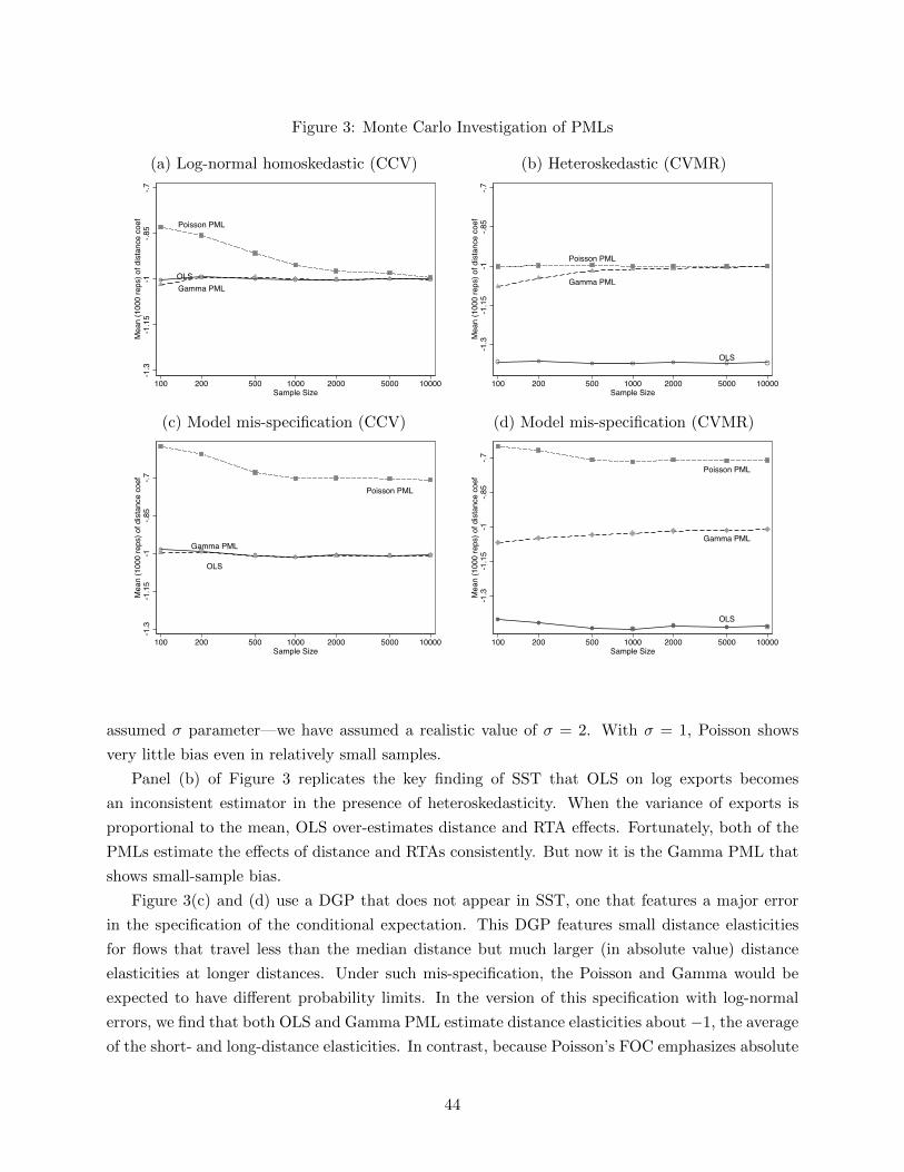
Figure 3: Monte Carlo Investigation of PMLs
(a) Log-normal homoskedastic (CCV) (b) Heteroskedastic (CVMR)
Poisson PML
Gamma PMLOLS
-1.3
-1.1
5-1
-.85
-.7M
ean
(100
0 re
ps) o
f dist
ance
coe
f
100 200 500 1000 2000 5000 10000Sample Size
Poisson PML
Gamma PML
OLS
-1.3
-1.1
5-1
-.85
-.7M
ean
(100
0 re
ps) o
f dist
ance
coe
f
100 200 500 1000 2000 5000 10000Sample Size
(c) Model mis-specification (CCV) (d) Model mis-specification (CVMR)
Poisson PML
Gamma PML
OLS
-1.3
-1.1
5-1
-.85
-.7M
ean
(100
0 re
ps) o
f dist
ance
coe
f
100 200 500 1000 2000 5000 10000Sample Size
Poisson PML
Gamma PML
OLS
-1.3
-1.1
5-1
-.85
-.7M
ean
(100
0 re
ps) o
f dist
ance
coe
f
100 200 500 1000 2000 5000 10000Sample Size
assumed σ parameter—we have assumed a realistic value of σ = 2. With σ = 1, Poisson shows
very little bias even in relatively small samples.
Panel (b) of Figure 3 replicates the key finding of SST that OLS on log exports becomes
an inconsistent estimator in the presence of heteroskedasticity. When the variance of exports is
proportional to the mean, OLS over-estimates distance and RTA effects. Fortunately, both of the
PMLs estimate the effects of distance and RTAs consistently. But now it is the Gamma PML that
shows small-sample bias.
Figure 3(c) and (d) use a DGP that does not appear in SST, one that features a major error
in the specification of the conditional expectation. This DGP features small distance elasticities
for flows that travel less than the median distance but much larger (in absolute value) distance
elasticities at longer distances. Under such mis-specification, the Poisson and Gamma would be
expected to have different probability limits. In the version of this specification with log-normal
errors, we find that both OLS and Gamma PML estimate distance elasticities about −1, the average
of the short- and long-distance elasticities. In contrast, because Poisson’s FOC emphasizes absolute
44
deviations, it puts more emphasis on the high-expected-trade observations, delivering an elasticity,
−0.7, that is much closer to the short-distance elasticity. The final simulation shown in Figure 3(d)
combines the CVMR error with the distance elasticity mis-specification. The two PML are hardly
changed compared to frame (c), but OLS now estimates the absolute distance elasticity to be over
1.3, as was the case in frame (b).
The Monte Carlo simulations also attest to the usefulness of estimating the MaMu regression.
We find that in the log-normal DGP that λ ≈ 2. On the other hand, under the CVMR DGP,
λ ≈ 1.6 with a range of 1.55 to 1.66 if there are 10,000 observations. Even though the MaMu
regression does not robustly estimate true λ, it appears to be a reliable method for distinguishing
between the two DGPs. Estimates of λ significantly below two were a near perfect predictor of a
CVMR DGP. 40
Our Monte Carlo results suggest that rather than selecting the Poisson PML as the single
“workhorse” estimator of gravity equations, it should be used as part of a robustness-exploring
ensemble that also includes OLS and Gamma PML. Upon comparing the results of each method,
we suggest the following conclusions be drawn.
1. If all three estimates are similar, then we can relax because the model appears to be well-
specified and η is approximately lognormal with a constant σ parameter.
2. If the Poisson and Gamma PML coefficients are similar to each other and both are distinct
from the OLS, then it is reasonable to conclude that heteroskedasticity is a problem and the
OLS estimates are unreliable.
3. If the Gamma and OLS coefficients on trade cost proxies are similar and the Poisson coeffi-
cients are smaller in absolute magnitude—as occurs in panels (a) and (c)—our simulations
suggest two possible interpretations.
(a) If the root mean squared error is large and sample size is not very large, this pattern
might be arising from small sample bias of the Poisson PML.
(b) If the sample size is large enough to dismiss small-sample bias, then trade cost elasticities
may be falling in absolute value as trade itself rises.
4. More generally, major divergence in large samples between Poisson and Gamma PML—as
exhibited in cases (c) and (d)—can signal model mis-specification.
5.2 Causes and consequences of zeros
The structural gravity models we have considered in this paper express trade as the multiple of
strictly positive variables. Hence, they do not naturally generate zero flows. Most actual trade data
sets exhibit substantial fractions of zeros, which become more frequent with disaggregation at the
40Specifically under log-normality, only 6 in 1,000 cases with a sample size of 10,000 did the MaMu test find λ < 2at the 5% significance. With CVMR errors, the MaMu test rejects λ = 2 in all repetitions.
45
firm or product level. Haveman and Hummels (2004) is an early paper tabulating the frequency
of zeros. Even at the country level, Helpman et al. (2008) report that country pairs that do not
trade with each other or trade in only one direction account for about half the observations. The
high frequency of zeros calls for two things. First, we need to adjust our trade models in order
to accommodate zeros since they are an important feature of the data. Second, we need to revise
our methods of estimation to allow for consistent estimates in the presence of a dependent variable
that takes on zeros frequently.
There a number of possible modifications to the structural gravity model to incorporate zeros.
The simplest approach is to assume that zeros are simply a data recording issue, i.e. that there are
no “structural zeros” but only “statistical zeros.” This would occur due to rounding or declaration
thresholds. Structural models of zeros mainly work by adding a fixed cost of exporting a positive
amount from i to n. In the Chaney (2008) model, fixed costs are not enough to cause zeros because
of the assumption of a continuum of firms with unbounded productivity. Helpman et al. (2008)
truncate the productivity distribution and this leads to zeros for some dyads. In contrast, Eaton
et al. (2012) generate zeros by abandoning the assumption of a continuum of firms. With a finite
number of draws there will be (in realization) a maximum productivity firm even if the productivity
distribution has infinite upper support. If the most productive firm from i cannot export profitably
to n, then there will be no trade between these countries. Also, as we noted in 2.3, with a finite
number of consumers, each selecting a single supplier, there will be realizations of the random
utility model in which two countries do not trade.
These models all share the feature that zeros are more likely when bilateral trade is expected
to be low, i.e. between distant and/or small countries.41 Unobserved trade costs will endogenously
create zeros. When taking logs of the zeros we remove those observations. That leads to the
systematic selection bias illustrated in Table 3. For this reason, it is important to determine
which estimators can deliver good results even when zeros are endogenous component of the data
generating process.
We now proceed to consider several candidate estimating methods prior to judging them using a
Monte Carlo simulation. One commonly used method that does not deserve Monte Carlo treatment
is the practice of adding one to observed exports and then taking logs. This gives a lower limit of 0
so Tobit is sometimes applied. The method should be avoided because results depend on the units
of measurement. Thus, the interpretation of coefficients as elasticities is lost. In the web appendix
we show that distance elasticities range from −1.93 to −0.09 as we change the exports units from
dollars to billions of dollars. The estimated impact of common currencies switches from negative
and significant to positive and significant simply by changing units from millions to billions.
Eaton and Tamura (1994) developed an early solution to incorporate zeros that can be thought
of as a model of ln(a + Xni) where instead of arbitrarily setting a = 1, it is instead treated as a
parameter to be estimated. One could think of a as a fixed amount of trade that “melts” away
before the trade flow is measured by government. More formally, the method, which we refer to as
41Baldwin and Harrigan (2011) find this pattern of zeros in the US product-level trade data.
46
ET Tobit, defines a strictly positive latent variable X∗ni and a threshold a such that when X∗ni > a
we observe Xni = X∗ni − a and when X∗ni ≤ a we observe Xni = 0. Unfortunately, a lacks a
compelling structural interpretation. Another drawback of ET Tobit is that it is not a “canned”
program.
Eaton and Kortum (2001) propose another method that has the advantage of being both easier
to implement and interpret. Suppose that there is minimum level of trade, a, such that if “ideal”
trade, X∗ni, falls below a we observe Xni = 0 but otherwise we observe Xni = X∗ni. Each an is
estimated as the minimum Xni for a given n, which we denote as Xni. To estimate the model, all
the observed zeros in Xni are replaced with Xni and the new bottom-coded lnXni is the dependent
variable in a Tobit command that allows for a user-specified lower limit of lnXni. The EK Tobit,
as we will refer to this method, has the advantages of (a) not requiring exclusion restrictions, (b)
being easily estimable using Stata’s intreg command.
Helpman et al. (2008) take a Heckman-based approach to zeros. This involves first using probit
to estimate the probability that n imports a positive amount from i. The second step estimates
the gravity equation on the positive-flow observations including a selection correction. A challenge,
common to Heckman-based methods, is that it is difficult to find an exclusion restriction. Thus, one
ideally would like to use a variable in the export status probit that theory tells you can be excluded
from the gravity equation. Since both equations have country fixed effects, this variable needs to
be dyadic in nature. Helpman et al. (2008) consider overlap in religion and the product of dummies
for low entry barriers in countries i and n. While their model deals with zeros, the main focus of
their method is to remove the effect of the extensive firm margin so as to estimate intensive margin
effects. Thus, they are designed to uncover a different set of parameters than the other approaches
which estimate coefficients that combine extensive and intensive margins. Consequently, we omit
this method from the Monte Carlo simulations.
In any model that abandons the continuum assumption, the market shares πni that appear
in all structural gravity formulations should be reinterpreted as expectations. For a wide class
of models featuring finite numbers of buyers and sellers, we conjecture that it is reasonable to
stipulate E(Xni/Xn) = πni. In that case, the appropriate estimator is the Multinomial PML, a
solution advanced by Eaton et al. (2012) for the case of a finite numbers of firms. Fortunately,
as proven in unpublished notes by Sebastian Sotelo, the Multinomial PML can be estimated by
applying the poisson command to the market share variable Xni/Xn, along with country-specific
fixed effects.42 By using a dependent variable that divides raw trade by the importing country’s
total expenditure, the MNPML accords less importance to large levels of trade. This is because the
biggest dyadic flows tend to be imported by country’s with large aggregate expenditures. Shares
prevent this dependent variable from obtaining values over one.43
Since one of the original draws of the Poisson PML method was that it allows for easy incorpo-
42The Eaton et al. (2012) specification also includes country dummies interacted with a dummy for trade with self(n = i).
43The potential drawback is the maintained assumption of an expenditure elasticity of one. In gravity modelsfeaturing quasi-linear utility for instance, that elasticity is zero.
47

ration of zeros, we will consider the performance of both Poisson and Gamma PML in the Monte
Carlo simulation. Previous simulation evidence had produced mixed results. While Poisson PML
performs well in Santos Silva and Tenreyro (2006), their simulation uses statistical zeros, obtained
via rounding. Santos Silva and Tenreyro (2011) propose a mixture model to generate zeros. Total
bilateral exports are given as the product of a random number of exporters and a random level of
exports per firm. Santos Silva and Tenreyro (2011) set the share of zeros between 62% and 83%
by choosing high variance parameters for the assumed negative binomial count distribution deter-
mining the number of exporters. Even with such high zero frequencies, they find both Poisson and
Gamma PML outperform alternatives such as linear-in-logs OLS (on the positives), log of one plus
exports, and the ET Tobit. These simulations make it clear that the mere presence of large shares
of zeros does not undermine the performance of PML estimators such as Poisson and Gamma.
The issue left unresolved by Santos Silva and Tenreyro (2011) is whether a DGP that followed
modern theory by explicitly featuring fixed costs might be problematic for the PML estimators. In
particular, the number of exporting firms should not be purely random but should instead depend
on trade costs and market sizes, just as the volume of exports does. Martin and Pham (2011)
consider DGPs involving threshold values and find that Tobit and Heckman methods outperform
the Poisson PML. However, as noted by Santos Silva and Tenreyro (2011), their DGP is not
multiplicative so it does not embed the fundamental problem of linear estimation in the presence
of heteroskedasticity.
We consider a DGP that takes as its starting point the structural gravity model. We make
a straightforward modification of the heterogeneous firms’ version of structural gravity seen in
section 2.3.2 so that it can generate zeroes. The simple idea is that profits for firm α from i
exporting to market n in the CES monopolistic competition model are given by xni(α)/σ − fn.
The threshold level of sales at which zero profits would be earned is x∗ni = σfn. Therefore if the
initial prediction for aggregate trade Xni falls below σfn then it would be impossible for any firm
to enter and break even. The result would be an observation of Xni = 0. Thus this data generating
process corresponds to the assumptions of the EK Tobit so long as the disturbances are log-normally
distributed.
We do not observe the market-specific entry costs but instead assume that fn is log-normal,
with mean and variance parameters chosen so as to replicate the 25% of zeroes in the DOTS data
for 2006 that we also used in the first Monte Carlo exercise of section 3. The procedure is also
very much in line with the first Monte Carlo, modified to generate and account for the zeros. The
assumed parameters on log distance and RTAs are maintained at −1 and 0.5 respectively, such that
τ−θni = exp(− ln Distni + 0.5RTAni)ηni. As before the model has an error term ηni that is assumed
to come from unobserved variable trade costs. We first specify ηni as a homoskedastic log-normal
term and then consider a second specification in which ηni is heteroskedastic, such that bilateral
trade has a constant variance to mean ratio (CVMR).
The contraction mapping algorithm generating simulated trade flows requires both i and n
incomes, combined with bilateral trade freeness, φni = τ−θni f−[ θ
σ−1−1]
n in this model. Based on our
48
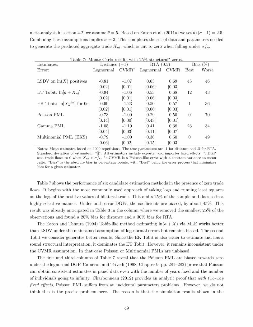
meta-analysis in section 4.2, we assume θ = 5. Based on Eaton et al. (2011a) we set θ/(σ−1) = 2.5.
Combining these assumptions implies σ = 3. This completes the set of data and parameters needed
to generate the predicted aggregate trade Xni, which is cut to zero when falling under σfn.
Table 7: Monte Carlo results with 25% structural? zeros.Estimates: Distance (−1) RTA (0.5) Bias (%)Error: Lognormal CVMR† Lognormal CVMR Best Worse
LSDV on ln(X) positives -0.81 -1.07 0.63 0.69 45 46[0.02] [0.01] [0.06] [0.03]
ET Tobit: ln[a+Xni] -0.94 -1.06 0.53 0.68 12 43[0.02] [0.01] [0.06] [0.03]
EK Tobit: ln[Xminn ] for 0s -0.99 -1.23 0.50 0.57 1 36
[0.02] [0.01] [0.06] [0.03]Poisson PML -0.73 -1.00 0.29 0.50 0 70
[0.14] [0.00] [0.43] [0.01]Gamma PML -1.05 -1.10 0.41 0.38 23 34
[0.04] [0.03] [0.11] [0.07]Multinomial PML (EKS) -0.79 -1.00 0.36 0.50 0 49
[0.06] [0.02] [0.15] [0.03]
Notes: Mean estimates based on 1000 repetitions. The true parameters are -1 for distance and .5 for RTA.Standard deviation of estimate in “[]”. All estimators include exporter and importer fixed effects. ?: DGPsets trade flows to 0 when Xni < σfn. †: CVMR is a Poisson-like error with a constant variance to meanratio. “Bias” is the absolute bias in percentage points, with “Best” being the error process that minimizesbias for a given estimator.
Table 7 shows the performance of six candidate estimation methods in the presence of zero trade
flows. It begins with the most commonly used approach of taking logs and running least squares
on the logs of the positive values of bilateral trade. This omits 25% of the sample and does so in a
highly selective manner. Under both error DGPs, the coefficients are biased, by about 45%. This
result was already anticipated in Table 3 in the column where we removed the smallest 25% of the
observations and found a 20% bias for distance and a 30% bias for RTA.
The Eaton and Tamura (1994) Tobit-like method estimating ln(a + X) via MLE works better
than LSDV under the maintained assumption of log-normal errors but remains biased. The second
Tobit we consider generates better results. Since the EK Tobit is also easier to estimate and has a
sound structural interpretation, it dominates the ET Tobit. However, it remains inconsistent under
the CVMR assumption. In that case Poisson or Multinomial PMLs are unbiased.
The first and third columns of Table 7 reveal that the Poisson PML are biased towards zero
under the lognormal DGP. Cameron and Trivedi (1998, Chapter 9, pp. 281–282) prove that Poisson
can obtain consistent estimates in panel data even with the number of years fixed and the number
of individuals going to infinity. Charbonneau (2012) provides an analytic proof that with two-way
fixed effects, Poisson PML suffers from an incidental parameters problems. However, we do not
think this is the precise problem here. The reason is that the simulation results shown in the
49
second and fourth columns show that Poisson with country effects is unbiased with CVMR errors.
Furthermore, the underestimates under log-normality appeared in the previous section even in the
absence of fixed effects. We conjecture that asymptotic properties of PPDV are not achieved due to
the high coefficient of variation in the simulation (calibrated on real data) and the need to estimate
(170− 1)× 2 = 338 importer and exporter effects.
Gamma PML does badly in the presence of the CVMR DGP and is even biased under the
log-normal assumption, where it had performed well in the previous simulation. Evidently, the
presence of zeros undermines its performance here. The most positive comment on Gamma PML
in the presence of structural zeros is that it exhibits the lowest worst-case bias (34%).
The selection of the appropriate estimator therefore appears to be contingent on the process
generating the error term. Under the CVMR we would want to use Poisson or Multinomial PML
but under log-normality EK Tobit is preferred. This points to the potential of the MaMu test for
log-normal errors introduced in the previous subsection. We ran 1000 repetitions of the MaMu test
for DGPs featuring varying shares of “structural zeros.” We estimated λ by applying OLS to the
logged squared residuals from the LSDV model. The results are reported in Figure 4.
Figure 4: Discriminating between different DGPs with structural zeros
log-normal prediction
LSDV: DOTS dataLSDV: TAP data
log-normal mean
CVMR mean
1.6
1.8
22.
2
1 5 10 25 50pct obs. missing
lam
bda
in M
aMu
test
Since LSDV excludes the zeros, there is reason to be doubtful that a MaMu test based on LSDV
errors would be unbiased. Figure 4 shows that as the percent of zeros increases, the expected value
of λ under log-normality departs from the true value of two. LSDV estimates give λ average 2.1
when the DGP is set to reflect the percent of zeros in the DOTS data (25%). Figure 4 shows that,
when the error term follows the CVMR DGP, λ is even worse at estimating the true λ, which in that
case is one. This is not due to zeros, as we found similar bias in the previous section without zeros.
Indeed, raising the share of zeros brings LSDV-based λ closer to the true value. More importantly,
as shown by the 99% confidence intervals on point, there is no overlap in the λ from the two error
structures.
In sum, while the MaMu test delivers biased estimates of λ under both DGPs, it can nevertheless
50
be used to distinguish between log-normal and CVMR with perfect accuracy in 1000 repetitions
of each DGP. A finding that λ ≥ 2 suggests EK Tobit is the estimator best matched to data
where zeros are generated by bilateral fixed entry costs. In contrast a λ significantly less than 2
militates for Poisson or Multinomial PML, with the preference going to MNPML since its worst-case
performance is better than Poisson.
A puzzle illustrated in Figure 4 is that the λ we obtain from regression on real data lie between
the simulation predictions. Export data on all goods from the 2006 IMF Direction of Trade Statis-
tics (DOTS) and manufactured goods in 2000 from the Trade and Production (TAP) data yield
strikingly similar estimates of 1.77 and 1.79, respectively. This could point to a mixture distribution
or to a process, such as the multinomial, that gives intermediate results.
5.3 Firm-level gravity, extensive and intensive margins
With the simultaneous emergence of the heterogenous firms modeling framework and firm-level
trade data, questions about the margins of adjustment to trade shocks have become important in
the literature. Researchers became interested in whether, after a rise in trade costs, or a fall in
final demand for instance, the global trade fall comes from all firms reducing their individual flows,
or on the contrary from exit of the smallest exporters. A recent example is Bricongne et al. (2012),
who apply this decomposition to the 2008–2009 trade collapse to find that most of the adjustment
came from existing firms cutting their shipments rather than from exit. There are however different
ways to decompose aggregate exports. To determine the most useful way, we need keep in mind
what different models predict.
The first extensive/intensive margin definition was proposed by Eaton et al. (2004), Hillberry
and Hummels (2008) and Bernard et al. (2007) and uses the identity that total exports equals the
number of active exporters multiplied by average shipments: Xni = Nnixni. The total elasticity
with respect to trade costs is therefore the sum of the elasticities of these two factors:44
∂ lnXni
∂ ln τni=∂ lnNni
∂ ln τni+∂ ln xni∂ ln τni
. (40)
This decomposition respects the traditional use of the extensive margin terminology as being the
change in the number of exporters, but the use of the intensive margin is unconventional. It
seems more in keeping with traditional usage to limit “intensive margin” changes to the individual
responses of firms following the change in trade costs. In (40), ∂ ln xni∂ ln τni
contains this effect, but
confounds it with the change in average shipments that comes from the changing composition of
exporters. We therefore want to split this term itself into two margins, the intensive and compo-
sitional. Using xni = 1G(α∗ni)
∫ α∗ni0 xni(α)g(α)dα, and using Leibniz rule as in Chaney (2008), it can
44Bernard et al. (2007), Mayer and Ottaviano (2007), and Bernard et al. (2011) have analyzed finer decompositions,taking into account multiproduct firms. Models of such firms are covered in this handbook by Melitz and Redding(2013).
51
be shown that:45
∂ lnXni
∂ ln τni=
∂ lnNni
∂ ln τni︸ ︷︷ ︸ext. margin
+1
xni
(∫ α∗ni
0
∂ lnxni(α)
∂ ln τnixni(α)
g(α)
G(α∗ni)dα
)︸ ︷︷ ︸
int. margin
+∂ lnG(α∗ni)
∂ lnα∗ni
∂ lnα∗ni∂ ln τni
(xni(α
∗ni)
xni− 1
)︸ ︷︷ ︸
compos. margin
. (41)
This 3-way decomposition nests the one proposed by Eaton et al. (2004), Hillberry and Hummels
(2008) and Bernard et al. (2007). In their decomposition, they simply add up the intensive and
compositional ones and call it intensive. It also nests the alternative decomposition proposed
by Chaney (2008), which is obtained when summing up our extensive and compositional and
calling it the extensive.46 The extensive and intensive margins in (40) have the classical respective
interpretations. The compositional margin is caused by the fact that new entrants/exitors do not
have the same productivity as the existing exporters. This margin is a function of the difference
between the marginal firm, with shipments xni(α∗ni) and the average shipment before the shock,
xni. This percentage difference is weighted in the overall effect by the change in the distribution of
firms associated with changes in trade costs (through changes in the cutoff).
Up to this point, the decomposition is purely definitional and does not depend on specifics
of the model nor on the assumed distribution of heterogeneity. Also important is that the two
first margins can be measured directly. The extensive margin is the elasticity of the number of
exporters (from i to n) with respect to trade costs, and the intensive margin is the elasticity of the
average shipments of the incumbent firms, that is the firms that were exporting before the shock
and still do afterwards.47 One can therefore calculate these two margins and back out the third
one as a residual to quantify the share of each. This “margins accounting” can in principle be
done independently of the underlying foundation for gravity, or even with models that do not have
closed-form solutions for those margins.
What should we expect for the value of the different margin elasticities? This will depend on
modeling assumptions naturally. There are two types of such assumptions that are usually made:
45The web appendix provides the derivation.46Chaney (2008) starts from aggregate trade Xni = Ni
∫ α∗ni
0xni(α)dG(α), and proceeds to decomposing between
the elasticity of shipments due to incumbent exporters, and the one caused by entrants/exitors:
∂ lnXni∂ ln τni
=τniXni
(Ni
∫ α∗ni
0
∂xni(α)
∂τnidG(α)
)+
τniXni
(Nixni(α
∗ni)g(α∗ni)
∂α∗ni∂τni
).
47Incumbents is a slight abuse of language here. Strictly speaking, the relevant set of firms in the model is the oneof firms that fall below the cost cutoff both before and after the trade cost shock, and therefore is defined in termsof productivity draw, rather than on initial presence in the market.
52
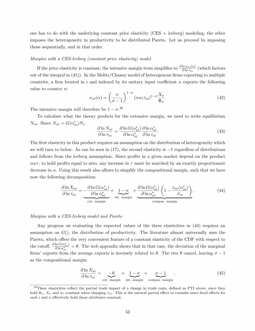
one has to do with the underlying constant price elasticity (CES + iceberg) modeling, the other
imposes the heterogeneity in productivity to be distributed Pareto. Let us proceed by imposing
those sequentially, and in that order.
Margins with a CES-Iceberg (constant price elasticity) model
If the price elasticity is constant, the intensive margin term simplifies to ∂ lnxni(α)∂ ln τni
(which factors
out of the integral in (41)). In the Melitz/Chaney model of heterogenous firms exporting to multiple
countries, a firm located in i and indexed by its unitary input coefficient α exports the following
value to country n:
xni(α) =
(σ
σ − 1
)1−σ(αwiτni)
1−σXn
Φn. (42)
The intensive margin will therefore be 1− σ.48
To calculate what the theory predicts for the extensive margin, we need to write equilibrium
Nni. Since Nni = G(α∗ni)Ni,∂ lnNni
∂ ln τni=∂ lnG(α∗ni)
∂ lnα∗ni
∂ lnα∗ni∂ ln τni
. (43)
The first elasticity in this product requires an assumption on the distribution of heterogeneity which
we will turn to below. As can be seen in (17), the second elasticity is −1 regardless of distributions
and follows from the iceberg assumption. Since profits in a given market depend on the product
αwτ , to hold profits equal to zero, any increase in τ must be matched by an exactly proportionate
decrease in α. Using this result also allows to simplify the compositional margin, such that we have
now the following decomposition:
∂ lnXni
∂ ln τni= −∂ lnG(α∗ni)
∂ lnα∗ni︸ ︷︷ ︸ext. margin
+ 1− σ︸ ︷︷ ︸int. margin
+∂ lnG(α∗ni)
∂ lnα∗ni
(1− xni(α
∗ni)
xni
)︸ ︷︷ ︸
compos. margin
. (44)
Margins with a CES-Iceberg model and Pareto
Any progress on evaluating the expected values of the three elasticities in (44) requires an
assumption on G(), the distribution of productivity. The literature almost universally uses the
Pareto, which offers the very convenient feature of a constant elasticity of the CDF with respect to
the cutoff,∂ lnG(α∗ni)∂ lnα∗ni
= θ. The web appendix shows that in that case, the deviation of the marginal
firms’ exports from the average exports is inversely related to θ. The two θ cancel, leaving σ − 1
as the compositional margin:
∂ lnXni
∂ ln τni= −θ︸︷︷︸
ext. margin
+ 1− σ︸ ︷︷ ︸int. margin
+ σ − 1︸ ︷︷ ︸compos. margin
. (45)
48These elasticities reflect the partial trade impact of a change in trade costs, defined as PTI above, since theyhold Φn, Xn and wi constant when changing τni. This is the natural partial effect to consider since fixed effects foreach i and n effectively hold those attributes constant.
53
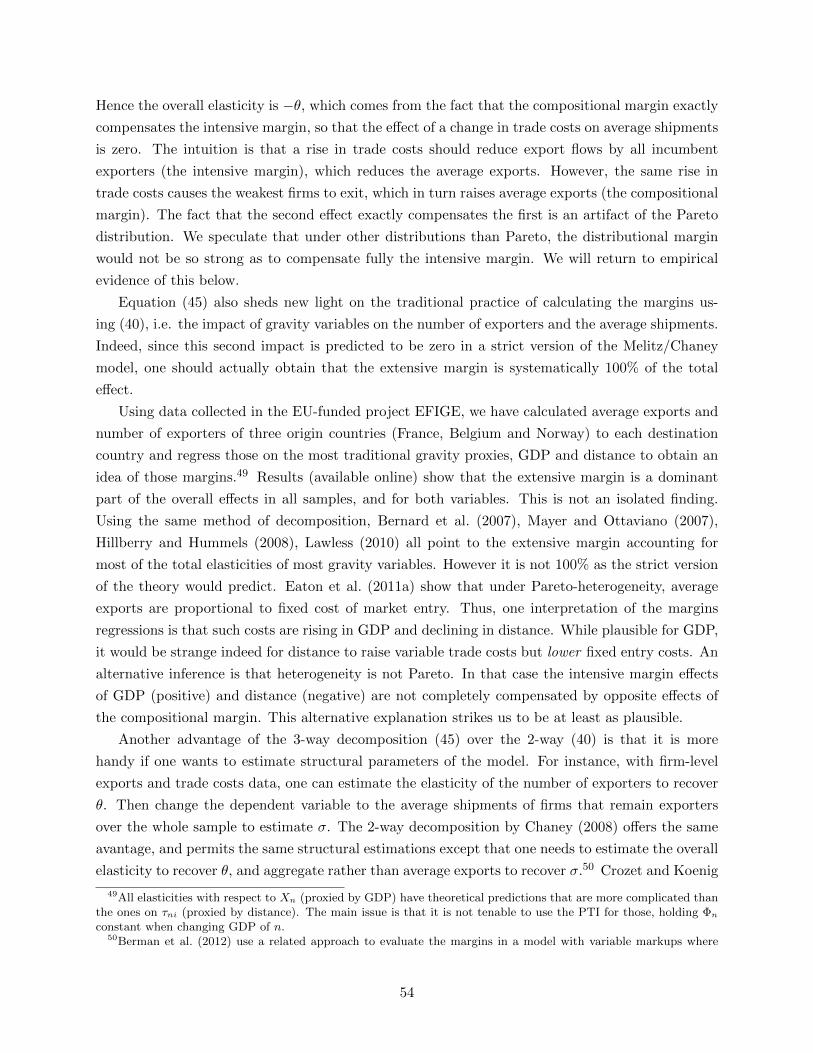
Hence the overall elasticity is −θ, which comes from the fact that the compositional margin exactly
compensates the intensive margin, so that the effect of a change in trade costs on average shipments
is zero. The intuition is that a rise in trade costs should reduce export flows by all incumbent
exporters (the intensive margin), which reduces the average exports. However, the same rise in
trade costs causes the weakest firms to exit, which in turn raises average exports (the compositional
margin). The fact that the second effect exactly compensates the first is an artifact of the Pareto
distribution. We speculate that under other distributions than Pareto, the distributional margin
would not be so strong as to compensate fully the intensive margin. We will return to empirical
evidence of this below.
Equation (45) also sheds new light on the traditional practice of calculating the margins us-
ing (40), i.e. the impact of gravity variables on the number of exporters and the average shipments.
Indeed, since this second impact is predicted to be zero in a strict version of the Melitz/Chaney
model, one should actually obtain that the extensive margin is systematically 100% of the total
effect.
Using data collected in the EU-funded project EFIGE, we have calculated average exports and
number of exporters of three origin countries (France, Belgium and Norway) to each destination
country and regress those on the most traditional gravity proxies, GDP and distance to obtain an
idea of those margins.49 Results (available online) show that the extensive margin is a dominant
part of the overall effects in all samples, and for both variables. This is not an isolated finding.
Using the same method of decomposition, Bernard et al. (2007), Mayer and Ottaviano (2007),
Hillberry and Hummels (2008), Lawless (2010) all point to the extensive margin accounting for
most of the total elasticities of most gravity variables. However it is not 100% as the strict version
of the theory would predict. Eaton et al. (2011a) show that under Pareto-heterogeneity, average
exports are proportional to fixed cost of market entry. Thus, one interpretation of the margins
regressions is that such costs are rising in GDP and declining in distance. While plausible for GDP,
it would be strange indeed for distance to raise variable trade costs but lower fixed entry costs. An
alternative inference is that heterogeneity is not Pareto. In that case the intensive margin effects
of GDP (positive) and distance (negative) are not completely compensated by opposite effects of
the compositional margin. This alternative explanation strikes us to be at least as plausible.
Another advantage of the 3-way decomposition (45) over the 2-way (40) is that it is more
handy if one wants to estimate structural parameters of the model. For instance, with firm-level
exports and trade costs data, one can estimate the elasticity of the number of exporters to recover
θ. Then change the dependent variable to the average shipments of firms that remain exporters
over the whole sample to estimate σ. The 2-way decomposition by Chaney (2008) offers the same
avantage, and permits the same structural estimations except that one needs to estimate the overall
elasticity to recover θ, and aggregate rather than average exports to recover σ.50 Crozet and Koenig
49All elasticities with respect to Xn (proxied by GDP) have theoretical predictions that are more complicated thanthe ones on τni (proxied by distance). The main issue is that it is not tenable to use the PTI for those, holding Φnconstant when changing GDP of n.
50Berman et al. (2012) use a related approach to evaluate the margins in a model with variable markups where
54

(2010) use firm-level regressions of the same theoretical setup to estimate the structural parameters
from the equations for export values, productivity distributions and export probabilities, so as to
calculate the Chaney (2008) margins. Interestingly, and in line with the arguments above, Crozet
and Koenig (2010) find the share of the extensive margin using Chaney’s method to be much smaller
than what the literature has found using the first method. Also, they do find a large variance in
the shares of the two margins across sectors, a finding hard to reconcile with the decomposition
method using (40).
While the intensive margin using the margins decomposition is one method to estimate the
parameter σ, there is a more direct way, using firm-level shipments. Firm-level trade data typically
takes the form of exports values reported by the national customs administration for each firm over
a certain number of year. While it would be very valuable to be able to put together several of those
national datasets, confidentiality issues make it very unlikely to happen any time soon. Taking logs
of (42), dropping the source country index, and adding a time dimension and a properly behaved
error term, one obtains
lnxnt(α) = (1− σ) ln
(σ
σ − 1
)+ (1− σ) ln(αtwt) + (1− σ) ln τnt + ln(Xnt/Φnt) + εnt(α). (46)
The first point to note is that there are two sources of identification for 1 − σ: one from the
cost component of the firm (αtwt), the other one from international price shifters (τnt). Let us
focus on τnt first. The regression will need to capture both some firm-time level determinant
and some destination-time one. It is quite clear from Equation (46) that no ideal structure of
fixed effects will work, since τnt and Xnt/Φnt vary along the same dimensions. One path is to
introduce firm-destination effects, that capture the time invariant determinants of αw and Xn/Φn,
but also any part of εnt(α) that does not change over time. The regression can then identify the
effect of τnt from the variation over time (the regression should also include proxies for changes in
demand of the destination and efficiency of the firm). Such changes in trade costs can come from
trade policy naturally, and there are databases (listed in the web appendix) which can be used
to measure changes in applied tariffs by different destination countries. Moreover, any bilateral
price shifter would in theory have the same impact: Freight rates for instance also reveal the trade
cost elasticity. Fitzgerald and Haller (2012) and Berman et al. (2012) estimate this elasticity using
firm-level shipments for Irish and French exports respectively. The price shifters in Fitzgerald and
Haller (2012) are the real exchange rate, and tariff changes from 2000 to 2004. The impact of
tariffs seems to be of the same order of magnitude as the aggregate literature, with an elasticity
around −5. Interestingly enough, the coefficient on the exchange rate is much lower, between 0.8
and 1, which is very similar to what Berman et al. (2012) find for French firms. This discrepancy
is reminiscent of findings in the aggregate literature.
An interesting case to consider for firm-level exports is when exports of a certain good originates
they don’t have closed-form solutions for the margins.
55
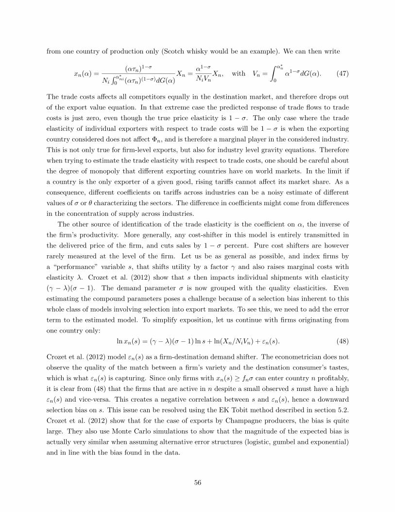
from one country of production only (Scotch whisky would be an example). We can then write
xn(α) =(ατn)1−σ
Ni
∫ α∗ni0 (ατn)(1−σ)dG(α)
Xn =α1−σ
NiVnXn, with Vn =
∫ α∗n
0α1−σdG(α). (47)
The trade costs affects all competitors equally in the destination market, and therefore drops out
of the export value equation. In that extreme case the predicted response of trade flows to trade
costs is just zero, even though the true price elasticity is 1 − σ. The only case where the trade
elasticity of individual exporters with respect to trade costs will be 1 − σ is when the exporting
country considered does not affect Φn, and is therefore a marginal player in the considered industry.
This is not only true for firm-level exports, but also for industry level gravity equations. Therefore
when trying to estimate the trade elasticity with respect to trade costs, one should be careful about
the degree of monopoly that different exporting countries have on world markets. In the limit if
a country is the only exporter of a given good, rising tariffs cannot affect its market share. As a
consequence, different coefficients on tariffs across industries can be a noisy estimate of different
values of σ or θ characterizing the sectors. The difference in coefficients might come from differences
in the concentration of supply across industries.
The other source of identification of the trade elasticity is the coefficient on α, the inverse of
the firm’s productivity. More generally, any cost-shifter in this model is entirely transmitted in
the delivered price of the firm, and cuts sales by 1 − σ percent. Pure cost shifters are however
rarely measured at the level of the firm. Let us be as general as possible, and index firms by
a “performance” variable s, that shifts utility by a factor γ and also raises marginal costs with
elasticity λ. Crozet et al. (2012) show that s then impacts individual shipments with elasticity
(γ − λ)(σ − 1). The demand parameter σ is now grouped with the quality elasticities. Even
estimating the compound parameters poses a challenge because of a selection bias inherent to this
whole class of models involving selection into export markets. To see this, we need to add the error
term to the estimated model. To simplify exposition, let us continue with firms originating from
one country only:
lnxn(s) = (γ − λ)(σ − 1) ln s+ ln(Xn/NiVn) + εn(s). (48)
Crozet et al. (2012) model εn(s) as a firm-destination demand shifter. The econometrician does not
observe the quality of the match between a firm’s variety and the destination consumer’s tastes,
which is what εn(s) is capturing. Since only firms with xn(s) ≥ fnσ can enter country n profitably,
it is clear from (48) that the firms that are active in n despite a small observed s must have a high
εn(s) and vice-versa. This creates a negative correlation between s and εn(s), hence a downward
selection bias on s. This issue can be resolved using the EK Tobit method described in section 5.2.
Crozet et al. (2012) show that for the case of exports by Champagne producers, the bias is quite
large. They also use Monte Carlo simulations to show that the magnitude of the expected bias is
actually very similar when assuming alternative error structures (logistic, gumbel and exponential)
and in line with the bias found in the data.
56
6 Directions for future research
Predicting which topics will turn out to be fertile for future research is never easy. However, based
on our assessment of the current set of problems and unresolved issues we offer three suggestions.
First, the underlying determinants of trade costs remain poorly understood. We are comfortable
with transport costs and tariffs yet we have reason to believe that neither are the most important
determinants of trade costs. First, distance effects are too large and have the wrong functional form
to be determined by freight costs. Second, border effects are large even along borders where tariffs
are very small. Other variables such as language and common currency have impacts on trade
that seem very large compared to any reasonable accounting of the costs that different languages
or different currencies impose. We believe that authors need to dig deeper to understand what
underlies these impacts.
The second topic that is attracting growing interest is the dynamics of trade. All the micro-
foundations of gravity that we examined are static models. They provide a derivation for a cross-
section but are questionable bases for panel estimation. This raises the econometric problem of how
to handle the evolution of trade over time in response to changes in trade costs. More fundamentally,
we need to think more about how to incorporate short-run capacity effects, learning, sunk costs
and other dynamic phenomena into the gravity equation framework.
The final topic has been lurking throughout our derivations of the micro-foundations. In every
model there came a point where very specific functional forms were imposed in order to maintain
tractability. The constant elasticity of substitution model for preferences is nearly ubiquitous.
Where it is less important, specific forms for heterogeneity (Frechet, Pareto) are often essential.
Finally theorists have often resorted to modeling firms using a continuum. Given the immense size
of firms like Airbus or Boeing, it is an embarrassment to stipulate that all firms have zero mass
and act as if they had no influence on the price index. Future research will need to devise ways to
investigate the consequences of departing from these assumptions and also ways to test whether the
data clearly reject the current set of restrictions customarily impose mainly for tractability rather
than realism.
7 Conclusions
The use of gravity equations to understand bilateral trade patterns exemplifies the beneficent roles
of empirical regularities in guiding theory development and theory in guiding estimation. Our
graphic displays of the systematic distance and size effects in trade data show the empirical appeal
of the gravity equation. We have catalogued the diverse set of microfoundations that deliver
“structural gravity,” our label for a formulation that matches stylized facts while calling for a more
sophisticated estimation approach than the one initially employed. After a quantitative summary
of 1000s of prior estimates, we illustrate the use of the structural form to determine the complete
trade and welfare impacts of policy changes. Our selective survey of topics at the frontier of current
research suggests that a great deal of interesting work lies ahead.
57

References
Abowd, J., Kramarz, F., Margolis, D., 1999. High wage workers and high wage firms. Econometrica
67 (2), 251–333.
Ahlfeldt, G., Redding, S., Sturm, D., Wolf, N., 2012. The economics of density: evidence from the
Berlin Wall, manuscript.
Anderson, J., 1979. A theoretical foundation for the gravity equation. The American Economic
Review 69 (1), 106–116.
Anderson, J., 2011. The Gravity Model. The Annual Review of Economics 3 (1), 133–160.
Anderson, J., Marcouiller, D., 2002. Insecurity and the pattern of trade: An empirical investigation.
Review of Economics and statistics 84 (2), 342–352.
Anderson, J., Yotov, Y., December 2010a. The Changing Incidence of Geography. American Eco-
nomic Review 100, 2157–2186.
Anderson, J., Yotov, Y., 2010b. Specialization: Pro-and Anti-Globalizing, 1990-2002. Working
Paper 16301, NBER.
Anderson, J. E., van Wincoop, E., 2003. Gravity with Gravitas: A Solution to the Border Puzzle.
The American Economic Review 93 (1), 170–192.
Anderson, J. E., Yotov, Y. V., February 2012. Gold Standard Gravity. Working Paper 17835,
NBER.
Anderson, S., De Palma, A., Thisse, J., 1992. Discrete choice theory of product differentiation.
MIT Press.
Arkolakis, C., Costinot, A., Donaldson, D., Rodrıguez-Clare, A., 2012a. The Elusive Pro-
Competitive Effects of Trade, manuscript.
Arkolakis, C., Costinot, A., Rodriguez-Clare, A., 2012b. New Trade Models, Same Old Gains?
American Economic Review 102 (1), 94–130.
Armington, P. S., 1969. A Theory of Demand for Products Distinguished by Place of Production.
Staff Papers - International Monetary Fund 16 (1), 159–178.
Baier, S., Bergstrand, J., 2007. Do free trade agreements actually increase members’ international
trade? Journal of International Economics 71 (1), 72–95.
Baier, S., Bergstrand, J., 2009. Bonus vetus OLS: A simple method for approximating international
trade-cost effects using the gravity equation. Journal of International Economics 77 (1), 77–85.
58
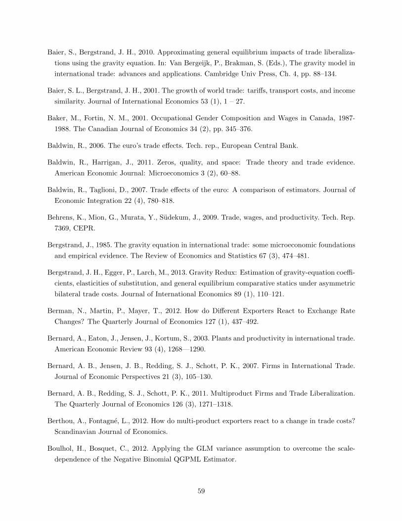
Baier, S., Bergstrand, J. H., 2010. Approximating general equilibrium impacts of trade liberaliza-
tions using the gravity equation. In: Van Bergeijk, P., Brakman, S. (Eds.), The gravity model in
international trade: advances and applications. Cambridge Univ Press, Ch. 4, pp. 88–134.
Baier, S. L., Bergstrand, J. H., 2001. The growth of world trade: tariffs, transport costs, and income
similarity. Journal of International Economics 53 (1), 1 – 27.
Baker, M., Fortin, N. M., 2001. Occupational Gender Composition and Wages in Canada, 1987-
1988. The Canadian Journal of Economics 34 (2), pp. 345–376.
Baldwin, R., 2006. The euro’s trade effects. Tech. rep., European Central Bank.
Baldwin, R., Harrigan, J., 2011. Zeros, quality, and space: Trade theory and trade evidence.
American Economic Journal: Microeconomics 3 (2), 60–88.
Baldwin, R., Taglioni, D., 2007. Trade effects of the euro: A comparison of estimators. Journal of
Economic Integration 22 (4), 780–818.
Behrens, K., Mion, G., Murata, Y., Sudekum, J., 2009. Trade, wages, and productivity. Tech. Rep.
7369, CEPR.
Bergstrand, J., 1985. The gravity equation in international trade: some microeconomic foundations
and empirical evidence. The Review of Economics and Statistics 67 (3), 474–481.
Bergstrand, J. H., Egger, P., Larch, M., 2013. Gravity Redux: Estimation of gravity-equation coeffi-
cients, elasticities of substitution, and general equilibrium comparative statics under asymmetric
bilateral trade costs. Journal of International Economics 89 (1), 110–121.
Berman, N., Martin, P., Mayer, T., 2012. How do Different Exporters React to Exchange Rate
Changes? The Quarterly Journal of Economics 127 (1), 437–492.
Bernard, A., Eaton, J., Jensen, J., Kortum, S., 2003. Plants and productivity in international trade.
American Economic Review 93 (4), 1268—1290.
Bernard, A. B., Jensen, J. B., Redding, S. J., Schott, P. K., 2007. Firms in International Trade.
Journal of Economic Perspectives 21 (3), 105–130.
Bernard, A. B., Redding, S. J., Schott, P. K., 2011. Multiproduct Firms and Trade Liberalization.
The Quarterly Journal of Economics 126 (3), 1271–1318.
Berthou, A., Fontagne, L., 2012. How do multi-product exporters react to a change in trade costs?
Scandinavian Journal of Economics.
Boulhol, H., Bosquet, C., 2012. Applying the GLM variance assumption to overcome the scale-
dependence of the Negative Binomial QGPML Estimator.
59

Bricongne, J.-C., Fontagne, L., Gaulier, G., Taglioni, D., Vicard, V., 2012. Firms and the global
crisis: French exports in the turmoil. Journal of International Economics 87 (1), 134 – 146.
Broda, C., Weinstein, D. E., 2006. Globalization and the Gains from Variety. Quarterly Journal of
Economics 121 (2), 541–585.
Caliendo, L., Parro, F., 2012. Estimates of the Trade and Welfare Effects of NAFTA. Tech. Rep.
18508, NBER.
Cameron, A., Trivedi, P., 1998. Regression analysis of count data. Cambridge Univ Press.
Chaney, T., 2008. Distorted Gravity: The Intensive and Extensive Margins of International Trade.
American Economic Review 98 (4), 1707–21.
Charbonneau, K. B., November 2012. Multiple Fixed Effects in Nonlinear Panel Data Models
Theory and Evidence, princeton mimeo.
Chen, H., Kondratowicz, M., Yi, K.-M., 2005. Vertical specialization and three facts about U.S.
international trade. The North American Journal of Economics and Finance 16 (1), 35–59.
Chen, N., Novy, D., 2011. Gravity, trade integration, and heterogeneity across industries. Journal
of International Economics Vol.85 (No.2), 206–221.
Cipollina, M., Salvatici, L., 2010. Reciprocal Trade Agreements in Gravity Models: A Meta-
Analysis. Review of International Economics 18 (1), 63–80.
Coeurdacier, N., Martin, P., 2009. The geography of asset trade and the euro: Insiders and outsiders.
Journal of the Japanese and International Economies 23 (2), 90–113.
Combes, P.-P., Lafourcade, M., Mayer, T., 2005. The trade-creating effects of business and social
networks: evidence from France. Journal of International Economics 66 (1), 1 – 29.
Costinot, A., Donaldson, D., Komunjer, I., 2012. What Goods Do Countries Trade? A Quantitative
Exploration of Ricardo’s Ideas. Review of Economic Studies 79 (2), 581–608.
Costinot, A., Rodriguez-Clare, A., 2013. Trade Theory with Numbers: Quantifying the Conse-
quences of Globalization. In: Helpman, E. (Ed.), Handbook of international economics. Vol. 4.
Elsevier.
Crozet, M., Head, K., Mayer, T., 2012. Quality sorting and trade: Firm-level evidence for French
wine. Review of Economic Studies 79 (2), 609 – 644.
Crozet, M., Koenig, P., 2010. Structural gravity equations with intensive and extensive margins.
Canadian Journal of Economics/Revue canadienne d’economique 43 (1), 41–62.
60
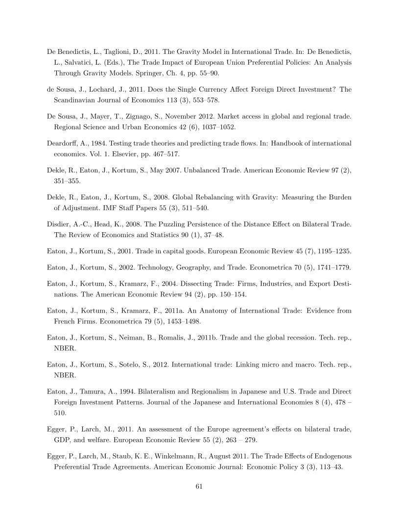
De Benedictis, L., Taglioni, D., 2011. The Gravity Model in International Trade. In: De Benedictis,
L., Salvatici, L. (Eds.), The Trade Impact of European Union Preferential Policies: An Analysis
Through Gravity Models. Springer, Ch. 4, pp. 55–90.
de Sousa, J., Lochard, J., 2011. Does the Single Currency Affect Foreign Direct Investment? The
Scandinavian Journal of Economics 113 (3), 553–578.
De Sousa, J., Mayer, T., Zignago, S., November 2012. Market access in global and regional trade.
Regional Science and Urban Economics 42 (6), 1037–1052.
Deardorff, A., 1984. Testing trade theories and predicting trade flows. In: Handbook of international
economics. Vol. 1. Elsevier, pp. 467–517.
Dekle, R., Eaton, J., Kortum, S., May 2007. Unbalanced Trade. American Economic Review 97 (2),
351–355.
Dekle, R., Eaton, J., Kortum, S., 2008. Global Rebalancing with Gravity: Measuring the Burden
of Adjustment. IMF Staff Papers 55 (3), 511–540.
Disdier, A.-C., Head, K., 2008. The Puzzling Persistence of the Distance Effect on Bilateral Trade.
The Review of Economics and Statistics 90 (1), 37–48.
Eaton, J., Kortum, S., 2001. Trade in capital goods. European Economic Review 45 (7), 1195–1235.
Eaton, J., Kortum, S., 2002. Technology, Geography, and Trade. Econometrica 70 (5), 1741–1779.
Eaton, J., Kortum, S., Kramarz, F., 2004. Dissecting Trade: Firms, Industries, and Export Desti-
nations. The American Economic Review 94 (2), pp. 150–154.
Eaton, J., Kortum, S., Kramarz, F., 2011a. An Anatomy of International Trade: Evidence from
French Firms. Econometrica 79 (5), 1453–1498.
Eaton, J., Kortum, S., Neiman, B., Romalis, J., 2011b. Trade and the global recession. Tech. rep.,
NBER.
Eaton, J., Kortum, S., Sotelo, S., 2012. International trade: Linking micro and macro. Tech. rep.,
NBER.
Eaton, J., Tamura, A., 1994. Bilateralism and Regionalism in Japanese and U.S. Trade and Direct
Foreign Investment Patterns. Journal of the Japanese and International Economies 8 (4), 478 –
510.
Egger, P., Larch, M., 2011. An assessment of the Europe agreement’s effects on bilateral trade,
GDP, and welfare. European Economic Review 55 (2), 263 – 279.
Egger, P., Larch, M., Staub, K. E., Winkelmann, R., August 2011. The Trade Effects of Endogenous
Preferential Trade Agreements. American Economic Journal: Economic Policy 3 (3), 113–43.
61
Erkel-Rousse, H., Mirza, D., 2002. Import price elasticities: reconsidering the evidence. Canadian
Journal of Economics 35 (2), 282–306.
Ethier, W. J., 1982. National and International Returns to Scale in the Modern Theory of Inter-
national Trade. The American Economic Review 72 (3), 389–405.
Fajgelbaum, P., Grossman, G., Helpman, E., 2011. Income Distribution, Product Quality, and
International Trade. Journal of Political Economy 119 (4), 721–765.
Fally, T., June 2012. Structural Gravity and Fixed Effects, university of Colorado note.
Feenstra, R., Obstfeld, M., Russ, K., 2010. In search of the Armington elasticity, university of
California-Davis, mimeo.
Feenstra, R. C., 1994. New Product Varieties and the Measurement of International Prices. The
American Economic Review 84 (1), 157–177.
Feenstra, R. C., 2003. A homothetic utility function for monopolistic competition models, without
constant price elasticity. Economics Letters 78 (1), 79–86.
Feenstra, R. C., 2004. Advanced International Trade: Theory and Evidence. Princeton University
Press, Princeton, New Jersey.
Feenstra, R. C., Markusen, J. R., Rose, A. K., 2001. Using the gravity equation to differentiate
among alternative theories of trade. Canadian Journal of Economics 34 (2), 430–447.
Fitzgerald, D., Haller, S., 2012. Exporters and Shocks, manuscript.
Frankel, J., 2010. The Estimated Trade Effects of the Euro: Why Are They Below Those From
Historical Monetary Unions Among Smaller Countries? In: Alesina, A., Giavazzi, F. (Eds.),
Europe and the Euro. University of Chicago Press, Ch. 5, pp. 169–212.
Frankel, J., Stein, E., Wei, S., 1997. Regional trading blocs in the world economic system. Institute
for International Economics (Washington, DC).
Glick, R., Rose, A. K., 2002. Does a currency union affect trade? The time-series evidence. Euro-
pean Economic Review 46 (6), 1125 – 1151.
Glick, R., Taylor, A. M., 2010. Collateral Damage: Trade Disruption and the Economic Impact of
War. Review of Economics and Statistics 92, 102–127.
Guimaraes, P., Portugal, P., 2010. A simple feasible alternative procedure to estimate models with
high-dimensional fixed effects. Stata Journal 10 (4), 628–649.
Hallak, J. C., 2006. Product quality and the direction of trade. Journal of International Economics
68 (1), 238 – 265.
62
Hanson, G., 2005. Market potential, increasing returns and geographic concentration. Journal of
International Economics 67 (1), 1–24.
Harrigan, J., 1996. Openness to Trade in Manufactures in the OECD. Journal of international
economics 40 (1-2), 23–39.
Haveman, J., Hummels, D., 2004. Alternative Hypotheses and the Volume of Trade: The Grav-
ity Equation and the Extent of Specialization. The Canadian Journal of Economics / Revue
canadienne d’Economique 37 (1), 199–218.
Head, K., Mayer, T., 2000. Non-Europe: the magnitude and causes of market fragmentation in the
EU. Review of World Economics 136 (2), 284–314.
Head, K., Mayer, T., 2004a. The empirics of agglomeration and trade. Handbook of regional and
urban economics 4, 2609–2669.
Head, K., Mayer, T., 2004b. Market potential and the location of Japanese investment in the
European Union. Review of Economics and Statistics 86 (4), 959–972.
Head, K., Mayer, T., Ries, J., 2009. How remote is the offshoring threat? European Economic
Review 53 (4), 429–444.
Head, K., Mayer, T., Ries, J., 2010. The erosion of colonial trade linkages after independence.
Journal of International Economics 81 (1), 1–14.
Head, K., Ries, J., 2001. Increasing returns versus national product differentiation as an explanation
for the pattern of US-Canada trade. American Economic Review 91 (4), 858–876.
Head, K., Ries, J., 2008. FDI as an Outcome of the Market for Corporate Control: Theory and
Evidence. Journal of International Economics 74 (1), 2–20.
Helliwell, J., 1998. How much do national borders matter? Brookings Inst Pr, Washington, D.C.
Helpman, E., Melitz, M., Rubinstein, Y., 2008. Estimating Trade Flows: Trading Partners and
Trading Volumes. Quarterly Journal of Economics 123 (2), 441–487.
Hillberry, R., Hummels, D., 2008. Trade responses to geographic frictions: A decomposition using
micro-data. European Economic Review 52 (3), 527 – 550.
Hortacu, A., Martinez-Jerez, F. A., Douglas, J., February 2009. The Geography of Trade in Online
Transactions: Evidence from eBay and Mercado Libre. American Economic Journal: Microeco-
nomics 1 (1), 53–74.
Hummels, D., 1999. Towards a Geography of Trade Costs. Tech. Rep. 17, GTAP Working Paper.
Imbs, J., Mejean, I., 2009. Elasticity optimism. Tech. rep., CEPR.
63
Isard, W., Peck, M., 1954. Location theory and international and interregional trade theory. The
Quarterly Journal of Economics 68 (1), 97–114.
Jacks, D., Meissner, C., Novy, D., 2008. Trade Costs, 1870-2000. The American Economic Review
98 (2), 529–534.
Krugman, P., 1979. Increasing Returns, Monopolistic Competition, and International Trade. Jour-
nal of International Economics 4, 469–479.
Krugman, P., 1995. Increasing returns, imperfect competition and the positive theory of interna-
tional trade. Handbook of international economics 3, 1243–1277.
Krugman, P., 1997. Development, geography, and economic theory. Vol. 6. The MIT Press.
Lai, H., Trefler, D., September 2002. The gains from trade with monopolistic competition: specifi-
cation, estimation, and mis-specification. Working Paper 9169, NBER.
Lawless, M., 2010. Deconstructing gravity: trade costs and extensive and intensive margins. Cana-
dian Journal of Economics/Revue canadienne d’economique 43 (4), 1149–1172.
Leamer, E., Levinsohn, J., 1995. International trade theory: the evidence. In: Handbook of inter-
national economics. Vol. 3. Elsevier, pp. 1339–1394.
Manning, W., Mullahy, J., 2001. Estimating log models: to transform or not to transform? Journal
of health economics 20 (4), 461–494.
Martin, P., Mayer, T., Thoenig, M., 2008. Make trade not war? Review of Economic Studies 75 (3),
865–900.
Martin, P., Mayer, T., Thoenig, M., 2012. The geography of conflicts and free trade agreements.
American Economic Journal: Macroeconomics 4 (4), 1–35.
Martin, P., Rey, H., 2004. Financial super-markets: size matters for asset trade. Journal of Inter-
national Economics 64 (2), 335 – 361.
Martin, W., Pham, C. S., 2011. Estimating the Gravity Model When Zero Trade Flows Are Fre-
quent. Tech. rep., World Bank.
Mayer, T., Ottaviano, G., 2007. The Happy Few: The Internationalisation of European firms.
Bruegel Blueprint Series.
McCallum, J., 1995. National borders matter: Canada-US regional trade patterns. The American
Economic Review 85 (3), 615–623.
Melitz, M., Ottaviano, G., 2008. Market Size, Trade, and Productivity. Review of Economic Studies
75 (1), 295–316.
64
Melitz, M. J., 2003. The Impact of Trade on Intra-Industry Reallocations and Aggregate Industry
Productivity. Econometrica 71 (6), 1695–1725.
Melitz, M. J., Redding, S. J., 2013. Within Industry Heterogeneity. In: Helpman, E. (Ed.), Hand-
book of International Economics. Vol. 4. Elsevier.
Novy, D., 2013. International Trade without CES: Estimating Translog Gravity. Journal of Inter-
national Economics 89 (?), –.
Okawa, Y., Van Wincoop, E., 2010. Gravity in international finance. Working Paper 7, Hong Kong
Institute for Monetary Research.
Okawa, Y., van Wincoop, E., 2012. Gravity in International Finance. Journal of International
Economics 87 (2), 205 – 215.
Ossa, R., 2011. A “New Trade” Theory of GATT/WTO Negotiations. Journal of Political Economy
119 (1), 122 – 152.
Ossa, R., 2012. Why Trade Matters After All. Working Paper 18113, NBER.
Ottaviano, G., Tabuchi, T., Thisse, J., 2002. Agglomeration And Trade Revisited. International
Economic Review 43 (2), 409.
Portes, R., Rey, H., 2005. The determinants of cross-border equity flows. Journal of International
Economics 65 (2), 269 – 296.
Portes, R., Rey, H., Oh, Y., 2001. Information and capital flows: The determinants of transactions in
financial assets. European Economic Review 45 (4a“6), 783 – 796, ¡ce:title¿15th Annual Congress
of the European Economic Association¡/ce:title¿.
Rauch, J. E., Trindade, V., 2002. Ethnic Chinese Networks In International Trade. The Review of
Economics and Statistics 84 (1), 116–130.
Redding, S., Venables, T., 2004. Economic Geography and International Inequality. Journal of
International Economics 62 (1), 53—82.
Romalis, J., 2007. Nafta’s And Cusfta’s Impact On International Trade. Review of Economics and
Statistics 89 (3), 416 – 435.
Rose, A., 2000. One money, one market: the effect of common currencies on trade. Economic policy
15 (30), 7–46.
Rose, A., 2004. Do We Really Know That the WTO Increases Trade? The American Economic
Review 94 (1), 98–114.
Santos Silva, J., Tenreyro, S., 2006. The log of gravity. The Review of Economics and Statistics
88 (4), 641–658.
65
Santos Silva, J., Tenreyro, S., 2010. Currency Unions in Prospect and Retrospect. Annu. Rev. Econ
2, 51–74.
Santos Silva, J., Tenreyro, S., August 2011. Further Simulation Evidence on the Performance of
the Poisson-PML Estimator. Economics Letters 112 (2), 220–222.
Savage, I. R., Deutsch, K. W., 1960. A Statistical Model of the Gross Analysis of Transaction
Flows. Econometrica 28 (3), pp. 551–572.
Simonovska, I., Waugh, M. E., February 2011. The Elasticity of Trade: Estimates and Evidence.
Working Paper 16796, NBER.
Tinbergen, J., 1962. Shaping the World Economy: Suggestions for an International Economic
Policy. Twentieth Century Fund, New-York.
Trefler, D., December 1995. The case of the missing trade and other mysteries. The American
Economic Review 85 (5), 1029–1046.
Wei, S.-J., April 1996. Intra-National versus International Trade: How Stubborn are Nations in
Global Integration? Working Paper 5531, NBER.
Wooldridge, J., 2010. Econometric analysis of cross section and panel data, second edition. The
MIT press.
66
Recommended