IBM COGNOS TM1 – IBM DO INTEGRATION Technique Document

IBM Analytic Solutions

by

2

Contents IBM COGNOS TM1 – IBM DO INTEGRATION ................................................................................ 1 CONTENTS............................................................................................................................................... 2

TECHNIQUE OVERVIEW .................................................................................................................... 3 PRODUCT REQUIREMENTS ............................................................................................................... 3 COMPONENT REQUIREMENTS ........................................................................................................ 3 PRELIMINARY STEPS .......................................................................................................................... 3

BUILD TM1 MODEL .................................................................................................................................. 3 BUILD DO MODEL ..................................................................................................................................... 4

PROCESS FLOW ..................................................................................................................................... 6

1. BUILD THE DO MAPPING CUBE (TM1) .................................................................................... 7 2. BUILD THE VIEW MAPPING CUBE (TM1) ............................................................................... 8 3. READING DATA FROM TM1 (JAVA, TM1)............................................................................. 10

3.1. INITIALIZE TM1 SERVER ................................................................................................................. 10 3.2. READ THE MAPPING CUBE FOR INPUTS TO DO ............................................................................... 11 3.3. READ THE TM1 OBJECTS ................................................................................................................. 11

4. SENDING DATA TO DO (JAVA, DO)......................................................................................... 12 5. OPTIMIZING THE DATA (JAVA, DO) ...................................................................................... 12

6. WRITING OPTIMIZED DATA TO TM1 (JAVA, DO, TM1) ................................................... 12 7. FULL EXAMPLE............................................................................................................................ 13

3

Technique Overview

This document explains a process that can be followed to integrate IBM Cognos TM1 and IBM Decision

Optimization (DO). This technique describes a way to use TM1 data structures such as Views or Subsets that

identify data in the TM1 model to be passed to DO as different, important parameters in an optimization process.

Logic and concepts are provided to be able to build a service from TM1 and DO API’s that will pull data from

TM1, send it to the DO engine with a DO model to be optimized and then return the optimized data to TM1.

The example shown throughout this document is based on the basic “gas” example from IBM ILOG DO

Optimization Studio 12.6.1.0, which can be imported through the File menu. It calculates how many units of each

gas should be produced from stocks of several components in order to maximize profit. The original example

model has been modified to use multiple types of input variables.

Product Requirements IBM Cognos TM1 (10.2.2 or greater)

IBM Cognos Configuration

IBM Cognos TM1 Server

IBM Cognos TM1 Architect or IBM Cognos TM1 Performance Modeler

IBM Decision Optimization (formal name??)

Local DO (e.g. IBM ILOG CPLEX Optimization Studio)

OR

DO on Cloud

Component Requirements

TM1 API

DO API

Preliminary Steps

Build TM1 model

An existing model can be used, or a new model can be built. If a new model is built, there are some

considerations mentioned throughout this document that may help in designing the model to facilitate the

integration with DO.

The model(s) contains data that is used as input to the DO model, and the optimized data is then returned to

be stored in the TM1 model(s). See Figure 1 for the example model.

4

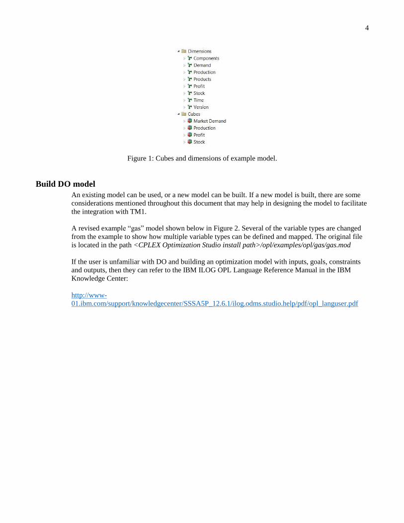
Figure 1: Cubes and dimensions of example model.

Build DO model

An existing model can be used, or a new model can be built. If a new model is built, there are some

considerations mentioned throughout this document that may help in designing the model to facilitate

the integration with TM1.

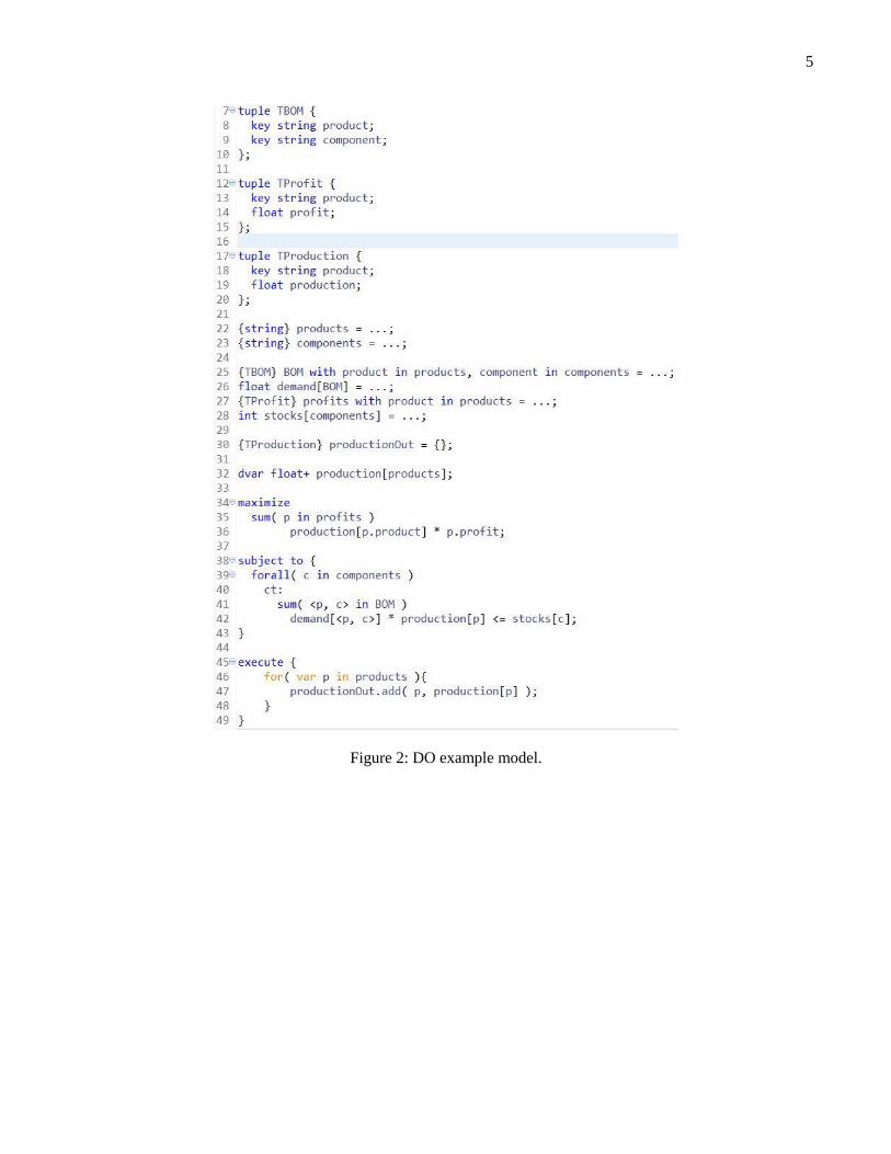
A revised example “gas” model shown below in Figure 2. Several of the variable types are changed

from the example to show how multiple variable types can be defined and mapped. The original file

is located in the path <CPLEX Optimization Studio install path>/opl/examples/opl/gas/gas.mod

If the user is unfamiliar with DO and building an optimization model with inputs, goals, constraints

and outputs, then they can refer to the IBM ILOG OPL Language Reference Manual in the IBM

Knowledge Center:

http://www-

01.ibm.com/support/knowledgecenter/SSSA5P_12.6.1/ilog.odms.studio.help/pdf/opl_languser.pdf

5

Figure 2: DO example model.

6

Process Flow

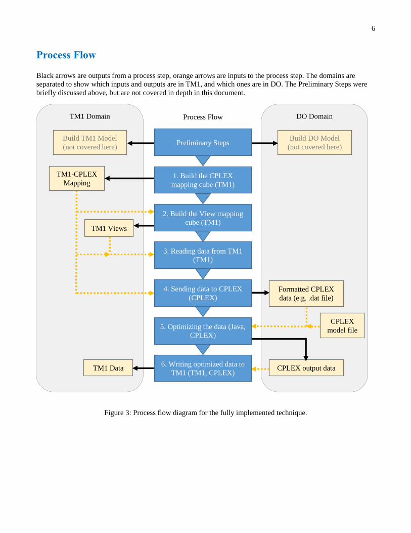
Black arrows are outputs from a process step, orange arrows are inputs to the process step. The domains are

separated to show which inputs and outputs are in TM1, and which ones are in DO. The Preliminary Steps were

briefly discussed above, but are not covered in depth in this document.

Figure 3: Process flow diagram for the fully implemented technique.

TM1 Domain

TM1 Views

TM1 Data

TM1-CPLEX

Mapping

Build TM1 Model

(not covered here)

DO Domain

Formatted CPLEX

data (e.g. .dat file)

CPLEX output data

CPLEX

model file

Build DO Model

(not covered here)

Process Flow

1. Build the CPLEX

mapping cube (TM1)

3. Reading data from TM1

(TM1)

5. Optimizing the data (Java,

CPLEX)

6. Writing optimized data to

TM1 (TM1, CPLEX)

2. Build the View mapping

cube (TM1)

4. Sending data to CPLEX

(CPLEX)

Preliminary Steps

7

1. Build the DO Mapping cube (TM1)

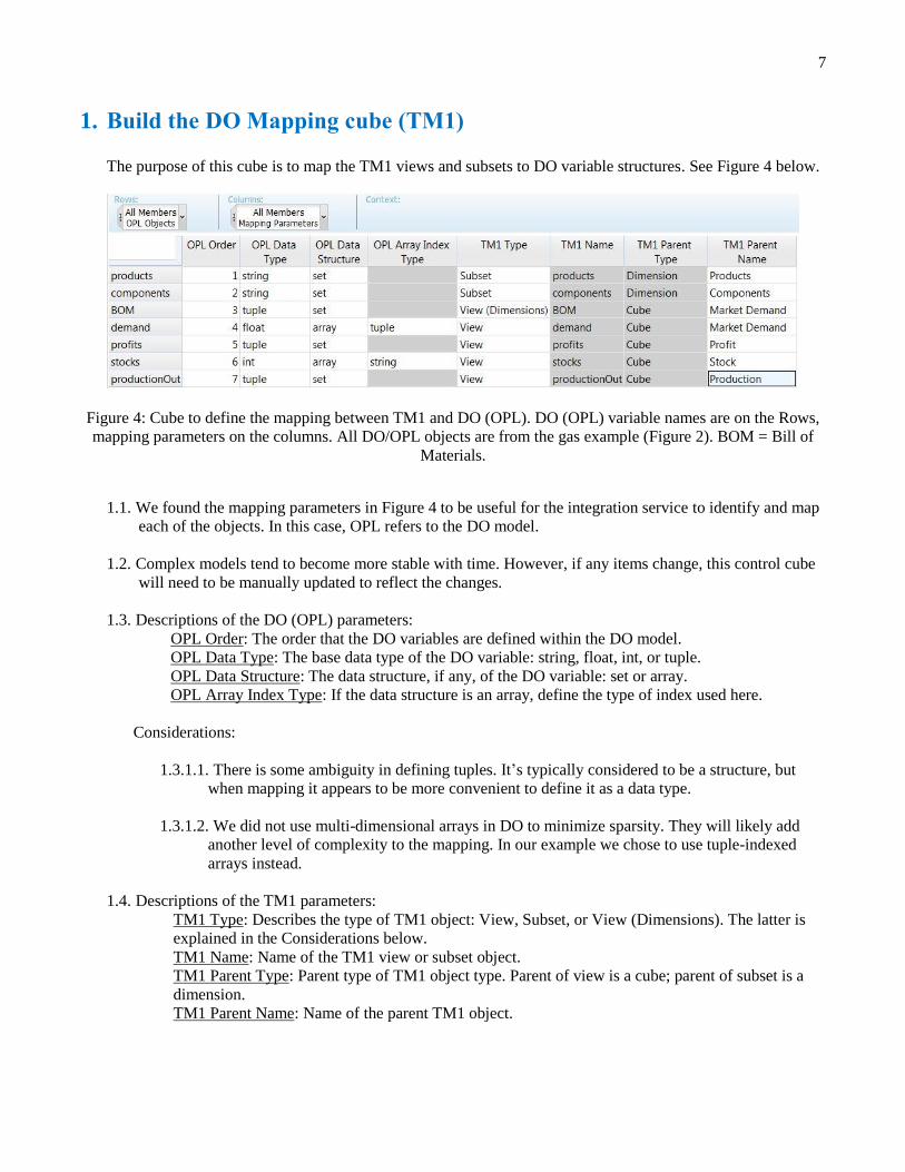
The purpose of this cube is to map the TM1 views and subsets to DO variable structures. See Figure 4 below.

Figure 4: Cube to define the mapping between TM1 and DO (OPL). DO (OPL) variable names are on the Rows,

mapping parameters on the columns. All DO/OPL objects are from the gas example (Figure 2). BOM = Bill of

Materials.

1.1. We found the mapping parameters in Figure 4 to be useful for the integration service to identify and map

each of the objects. In this case, OPL refers to the DO model.

1.2. Complex models tend to become more stable with time. However, if any items change, this control cube

will need to be manually updated to reflect the changes.

1.3. Descriptions of the DO (OPL) parameters:

OPL Order: The order that the DO variables are defined within the DO model.

OPL Data Type: The base data type of the DO variable: string, float, int, or tuple.

OPL Data Structure: The data structure, if any, of the DO variable: set or array.

OPL Array Index Type: If the data structure is an array, define the type of index used here.

Considerations:

1.3.1.1. There is some ambiguity in defining tuples. It’s typically considered to be a structure, but

when mapping it appears to be more convenient to define it as a data type.

1.3.1.2. We did not use multi-dimensional arrays in DO to minimize sparsity. They will likely add

another level of complexity to the mapping. In our example we chose to use tuple-indexed

arrays instead.

1.4. Descriptions of the TM1 parameters:

TM1 Type: Describes the type of TM1 object: View, Subset, or View (Dimensions). The latter is

explained in the Considerations below.

TM1 Name: Name of the TM1 view or subset object.

TM1 Parent Type: Parent type of TM1 object type. Parent of view is a cube; parent of subset is a

dimension.

TM1 Parent Name: Name of the parent TM1 object.

8

Considerations:

1.4.1.1. Views and subsets were the only TM1 types used because of their flexibility. It would be rare

for someone to use an entire cube or dimension, and even then they can define an appropriate

view or subset. They can capture any portion of a cube or dimension needed.

1.4.1.2. We found the type View (Dimensions) to be useful for tuple-indexed arrays, such as the OPL

object demand in Figure 4. The cube values are the values of the array in DO. The dimension

elements of the cube would be the tuple that indexes those values. When the tuples need to be

imported into DO without the values, then you can use the View (Dimensions) type.

1.4.1.3. It is worth noting that DO is case-sensitive, while TM1 is not. So while it is possible to have

two separate input variables as “products” and “Products” in DO, it is not possible to

distinguish between those when mapping in TM1. To make working with DO and TM1 easier,

DO input and output variables should be designed as if they are case-insensitive.

2. Build the View Mapping cube (TM1)

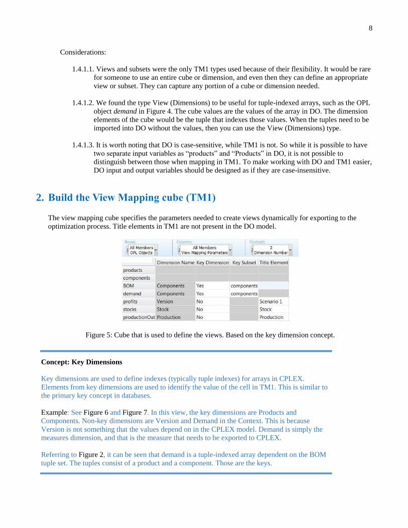
The view mapping cube specifies the parameters needed to create views dynamically for exporting to the

optimization process. Title elements in TM1 are not present in the DO model.

Figure 5: Cube that is used to define the views. Based on the key dimension concept.

Concept: Key Dimensions

Key dimensions are used to define indexes (typically tuple indexes) for arrays in CPLEX.

Elements from key dimensions are used to identify the value of the cell in TM1. This is similar to

the primary key concept in databases.

Example: See Figure 6 and Figure 7. In this view, the key dimensions are Products and

Components. Non-key dimensions are Version and Demand in the Context. This is because

Version is not something that the values depend on in the CPLEX model. Demand is simply the

measures dimension, and that is the measure that needs to be exported to CPLEX.

Referring to Figure 2, it can be seen that demand is a tuple-indexed array dependent on the BOM

tuple set. The tuples consist of a product and a component. Those are the keys.

9

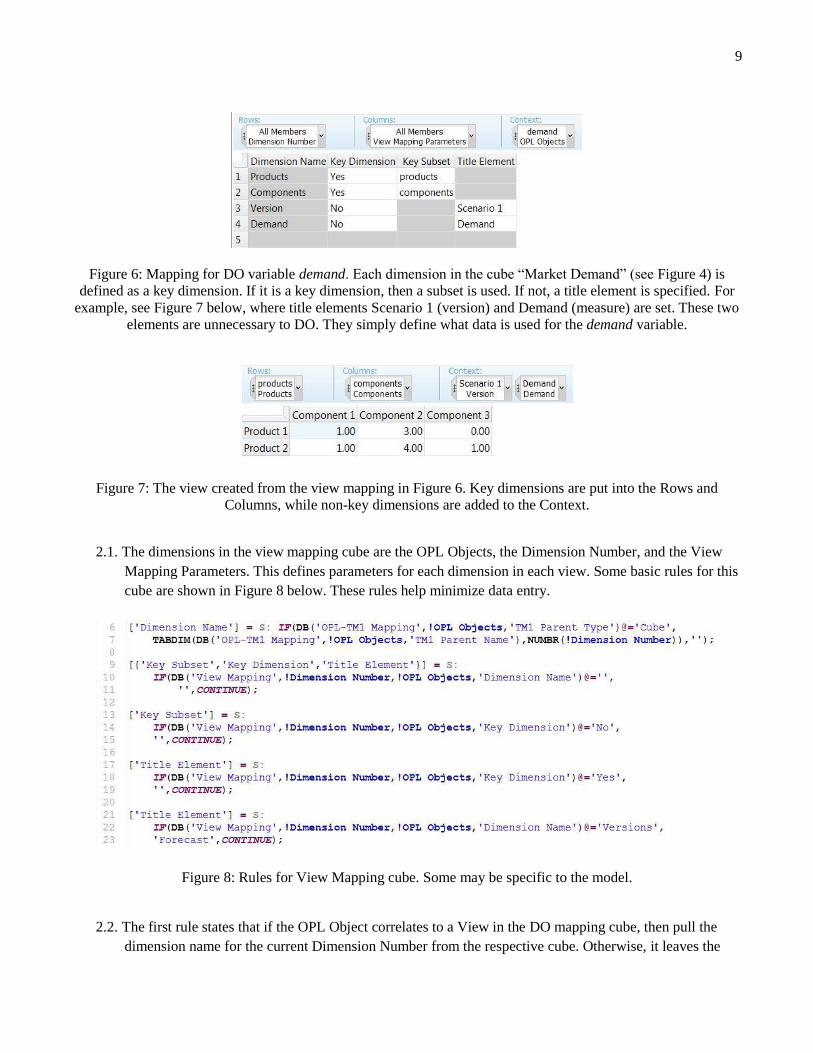
Figure 6: Mapping for DO variable demand. Each dimension in the cube “Market Demand” (see Figure 4) is

defined as a key dimension. If it is a key dimension, then a subset is used. If not, a title element is specified. For

example, see Figure 7 below, where title elements Scenario 1 (version) and Demand (measure) are set. These two

elements are unnecessary to DO. They simply define what data is used for the demand variable.

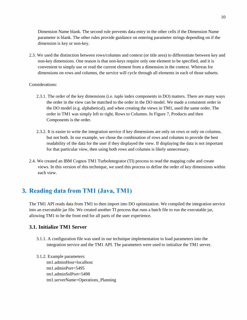
Figure 7: The view created from the view mapping in Figure 6. Key dimensions are put into the Rows and

Columns, while non-key dimensions are added to the Context.

2.1. The dimensions in the view mapping cube are the OPL Objects, the Dimension Number, and the View

Mapping Parameters. This defines parameters for each dimension in each view. Some basic rules for this

cube are shown in Figure 8 below. These rules help minimize data entry.

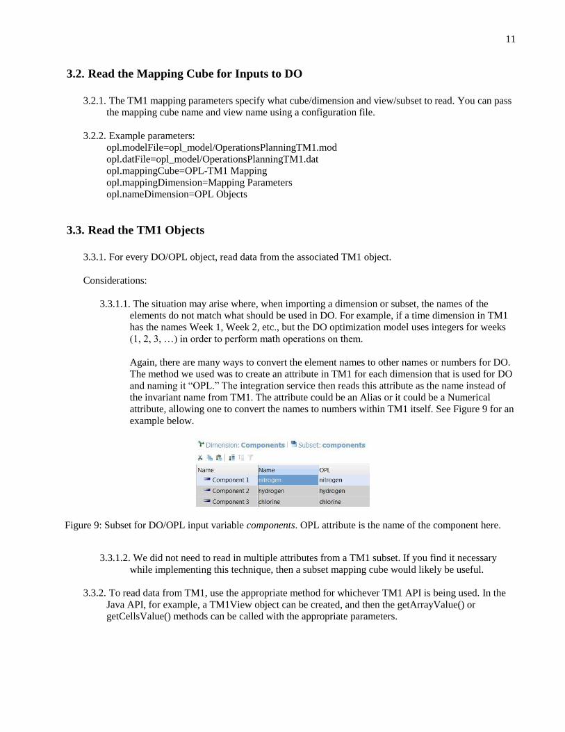
Figure 8: Rules for View Mapping cube. Some may be specific to the model.

2.2. The first rule states that if the OPL Object correlates to a View in the DO mapping cube, then pull the

dimension name for the current Dimension Number from the respective cube. Otherwise, it leaves the

10

Dimension Name blank. The second rule prevents data entry in the other cells if the Dimension Name

parameter is blank. The other rules provide guidance on entering parameter strings depending on if the

dimension is key or non-key.

2.3. We used the distinction between rows/columns and context (or title area) to differentiate between key and

non-key dimensions. One reason is that non-keys require only one element to be specified, and it is

convenient to simply use or read the current element from a dimension in the context. Whereas for

dimensions on rows and columns, the service will cycle through all elements in each of those subsets.

Considerations:

2.3.1. The order of the key dimensions (i.e. tuple index components in DO) matters. There are many ways

the order in the view can be matched to the order in the DO model. We made a consistent order in

the DO model (e.g. alphabetical), and when creating the views in TM1, used the same order. The

order in TM1 was simply left to right, Rows to Columns. In Figure 7, Products and then

Components is the order.

2.3.2. It is easier to write the integration service if key dimensions are only on rows or only on columns,

but not both. In our example, we chose the combination of rows and columns to provide the best

readability of the data for the user if they displayed the view. If displaying the data is not important

for that particular view, then using both rows and columns is likely unnecessary.

2.4. We created an IBM Cognos TM1 TurboIntegrator (TI) process to read the mapping cube and create

views. In this version of this technique, we used this process to define the order of key dimensions within

each view.

3. Reading data from TM1 (Java, TM1)

The TM1 API reads data from TM1 to then import into DO optimization. We compiled the integration service

into an executable jar file. We created another TI process that runs a batch file to run the executable jar,

allowing TM1 to be the front end for all parts of the user experience.

3.1. Initialize TM1 Server

3.1.1. A configuration file was used in our technique implementation to load parameters into the

integration service and the TM1 API. The parameters were used to initialize the TM1 server.

3.1.2. Example parameters:

tm1.adminHost=localhost

tm1.adminPort=5495

tm1.adminSslPort=5498

tm1.serverName=Operations_Planning

11

3.2. Read the Mapping Cube for Inputs to DO

3.2.1. The TM1 mapping parameters specify what cube/dimension and view/subset to read. You can pass

the mapping cube name and view name using a configuration file.

3.2.2. Example parameters:

opl.modelFile=opl_model/OperationsPlanningTM1.mod

opl.datFile=opl_model/OperationsPlanningTM1.dat

opl.mappingCube=OPL-TM1 Mapping

opl.mappingDimension=Mapping Parameters

opl.nameDimension=OPL Objects

3.3. Read the TM1 Objects

3.3.1. For every DO/OPL object, read data from the associated TM1 object.

Considerations:

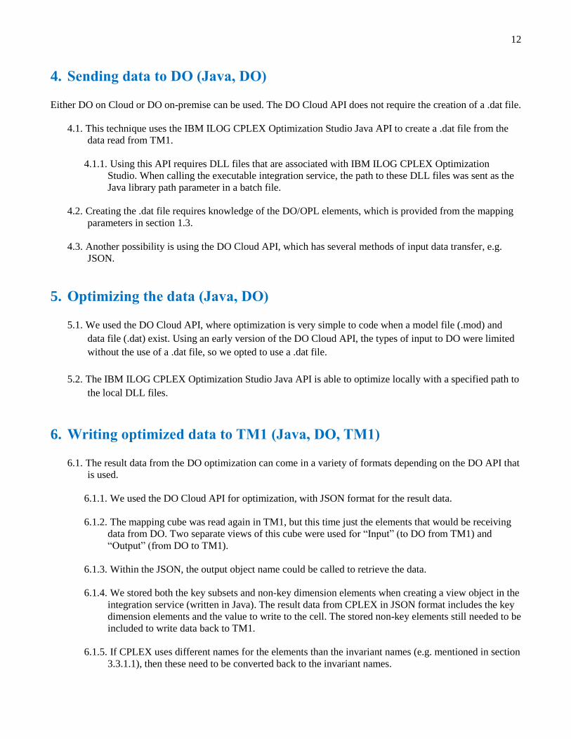
3.3.1.1. The situation may arise where, when importing a dimension or subset, the names of the

elements do not match what should be used in DO. For example, if a time dimension in TM1

has the names Week 1, Week 2, etc., but the DO optimization model uses integers for weeks

(1, 2, 3, …) in order to perform math operations on them.

Again, there are many ways to convert the element names to other names or numbers for DO.

The method we used was to create an attribute in TM1 for each dimension that is used for DO

and naming it “OPL.” The integration service then reads this attribute as the name instead of

the invariant name from TM1. The attribute could be an Alias or it could be a Numerical

attribute, allowing one to convert the names to numbers within TM1 itself. See Figure 9 for an

example below.

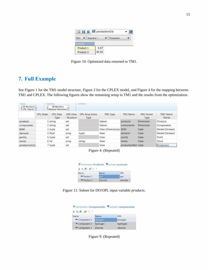
Figure 9: Subset for DO/OPL input variable components. OPL attribute is the name of the component here.

3.3.1.2. We did not need to read in multiple attributes from a TM1 subset. If you find it necessary

while implementing this technique, then a subset mapping cube would likely be useful.

3.3.2. To read data from TM1, use the appropriate method for whichever TM1 API is being used. In the

Java API, for example, a TM1View object can be created, and then the getArrayValue() or

getCellsValue() methods can be called with the appropriate parameters.

12

4. Sending data to DO (Java, DO)

Either DO on Cloud or DO on-premise can be used. The DO Cloud API does not require the creation of a .dat file.

4.1. This technique uses the IBM ILOG CPLEX Optimization Studio Java API to create a .dat file from the

data read from TM1.

4.1.1. Using this API requires DLL files that are associated with IBM ILOG CPLEX Optimization

Studio. When calling the executable integration service, the path to these DLL files was sent as the

Java library path parameter in a batch file.

4.2. Creating the .dat file requires knowledge of the DO/OPL elements, which is provided from the mapping

parameters in section 1.3.

4.3. Another possibility is using the DO Cloud API, which has several methods of input data transfer, e.g.

JSON.

5. Optimizing the data (Java, DO)

5.1. We used the DO Cloud API, where optimization is very simple to code when a model file (.mod) and

data file (.dat) exist. Using an early version of the DO Cloud API, the types of input to DO were limited

without the use of a .dat file, so we opted to use a .dat file.

5.2. The IBM ILOG CPLEX Optimization Studio Java API is able to optimize locally with a specified path to

the local DLL files.

6. Writing optimized data to TM1 (Java, DO, TM1)

6.1. The result data from the DO optimization can come in a variety of formats depending on the DO API that

is used.

6.1.1. We used the DO Cloud API for optimization, with JSON format for the result data.

6.1.2. The mapping cube was read again in TM1, but this time just the elements that would be receiving

data from DO. Two separate views of this cube were used for “Input” (to DO from TM1) and

“Output” (from DO to TM1).

6.1.3. Within the JSON, the output object name could be called to retrieve the data.

6.1.4. We stored both the key subsets and non-key dimension elements when creating a view object in the

integration service (written in Java). The result data from CPLEX in JSON format includes the key

dimension elements and the value to write to the cell. The stored non-key elements still needed to be

included to write data back to TM1.

6.1.5. If CPLEX uses different names for the elements than the invariant names (e.g. mentioned in section

3.3.1.1), then these need to be converted back to the invariant names.

13

Figure 10: Optimized data returned to TM1.

7. Full Example

See Figure 1 for the TM1 model structure, Figure 2 for the CPLEX model, and Figure 4 for the mapping between

TM1 and CPLEX. The following figures show the remaining setup in TM1 and the results from the optimization.

Figure 4: (Repeated)

Figure 11: Subset for DO/OPL input variable products.

Figure 9: (Repeated)

14

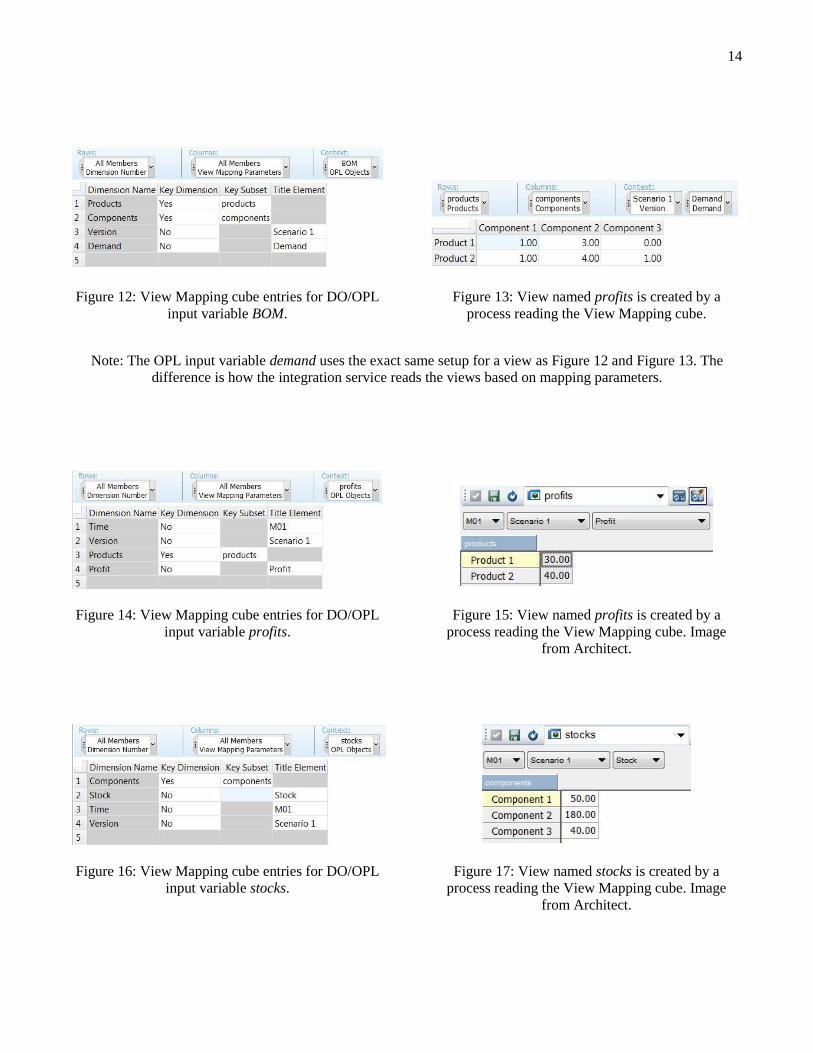
Figure 12: View Mapping cube entries for DO/OPL

input variable BOM.

Figure 13: View named profits is created by a

process reading the View Mapping cube.

Note: The OPL input variable demand uses the exact same setup for a view as Figure 12 and Figure 13. The

difference is how the integration service reads the views based on mapping parameters.

Figure 14: View Mapping cube entries for DO/OPL

input variable profits.

Figure 15: View named profits is created by a

process reading the View Mapping cube. Image

from Architect.

Figure 16: View Mapping cube entries for DO/OPL

input variable stocks.

Figure 17: View named stocks is created by a

process reading the View Mapping cube. Image

from Architect.

15

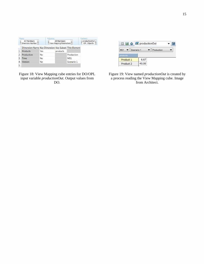
Figure 18: View Mapping cube entries for DO/OPL

input variable productionOut. Output values from

DO.

Figure 19: View named productionOut is created by

a process reading the View Mapping cube. Image

from Architect.

16

Licensed Materials – Property of IBM Corp. © Copyright IBM Corp. 2015

The Samples are owned by IBM and are copyrighted and licensed, not sold. They are licensed under the terms of

the International License Agreement for Non-Warranted Programs, which you accepted prior to downloading the

content from IBM developerWorks web site (https://www.ibm.com/developerworks/).

See the complete license terms at:

http://www-03.ibm.com/software/sla/sladb.nsf/pdf/ilan/$file/ilan_en.pdf

By using the Samples, you agree to these terms.