1

INFLUENCE OF BACKFILL SLOPE ON DYNAMIC RESPONSE OF FLEXIBLE

RETAINING STRUCTURES

Sandra Cristina Miranda Reis Lobo

Instituto Superior Técnico, Department of Civil Engineering

Abstract: Interaction between earth retaining structures and surrounding soil is a complex phenomenon for

both static and seismic loading. In the present paper a brief review of available methodologies for the design

of flexible retaining structures is done, for the seismic load, with a special focus on dynamic numerical

methods.

The seismic performance of a retaining wall depends on the total pressures (i.e., static plus dynamic

pressures) that act on it during the earthquake. Pseudostatic analysis are used in current practice to

estimate seismically induced wall pressures, and the wall is designed to resist those pressures without

failing or causing failure of the surrounding soil.

The present document aims to study the behaviour of a flexible braced retaining structure under the seismic

action. 2D numerical analyses using the finite element method were performed to study the response of

flexible retaining wall using SOFiSTiK FE software.

The parametric studies illustrate the effects of the backfill slope and intensity of seismic acceleration on the

stress field, struts forces, displacements and on the design of reinforced retaining walls.

Keywords: Seismic Action, Dynamics, nonlinear analysis, Retaining wall structure, SOFiSTiK.

1. INTRODUCTION

Deep excavations are widely used in urban areas for the development of underground space, e.g. subway

stations, basements for high-rise buildings, underground car parks, etc.. However, the excavation process

inevitably changes the ground’s stress state and may cause significant wall deformations and ground

movements. Observations of the performance of retaining structures in recent earthquakes show that

earthquakes have caused permanent deformations in some cases these deformations were negligible; in

others they have caused significant damage.

This study was undertaken to develop a better understanding of the dynamic performance for retaining

walls, with different backfill inclination and with different intensities of accelerogram.

2. GROUND RESPONSE ANALYSES

There are various methods to analyse retaining wall under seismic loads. The methods used in defining the

dynamic analysis of retaining walls may be categorized into two groups:

pseudo-static methods: these are simplified methods for seismic design, in which the effects of

earthquakes are represented by vertical and/or horizontal accelerations constant throughout the

height of the supported field;

2

dynamic methods: methods that take into account, approximately, dynamic response of the

structure and supported soil, translated by seismic coefficients variables.

The pseudo-static method normally to estimate the active thrust used is the Mononobe-Okabe method. This

method computes the dynamic pressure on support structures, being an extension of the Coulomb theory.

Mononobe-Okabe (M-O) method is still employed as the first option to estimate lateral earth pressures

during earthquakes by geotechnical engineers.

The response of the structure to seismic phenomena is always a dynamic response. Two and three-

dimensional ground response analyses are usually performed using dynamic finite-element analysis. These

analyses can be performed using equivalent linear or nonlinear approaches. The numerical model used is

based on time history dynamic 2D analysis using SOFiSTiK finite element analysis software.

3. DYNAMIC SOIL PROPERTIES

The mechanical behaviour of soils can be quite complex under seismic loading conditions.

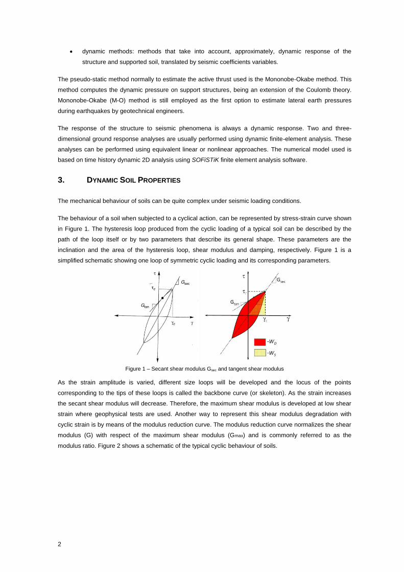
The behaviour of a soil when subjected to a cyclical action, can be represented by stress-strain curve shown

in Figure 1. The hysteresis loop produced from the cyclic loading of a typical soil can be described by the

path of the loop itself or by two parameters that describe its general shape. These parameters are the

inclination and the area of the hysteresis loop, shear modulus and damping, respectively. Figure 1 is a

simplified schematic showing one loop of symmetric cyclic loading and its corresponding parameters.

Figure 1 – Secant shear modulus Gsec and tangent shear modulus

As the strain amplitude is varied, different size loops will be developed and the locus of the points

corresponding to the tips of these loops is called the backbone curve (or skeleton). As the strain increases

the secant shear modulus will decrease. Therefore, the maximum shear modulus is developed at low shear

strain where geophysical tests are used. Another way to represent this shear modulus degradation with

cyclic strain is by means of the modulus reduction curve. The modulus reduction curve normalizes the shear

modulus (G) with respect of the maximum shear modulus (Gmax) and is commonly referred to as the

modulus ratio. Figure 2 shows a schematic of the typical cyclic behaviour of soils.

3

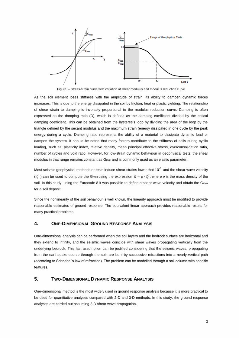
Figure – Stress-strain curve with variation of shear modulus and modulus reduction curve

As the soil element loses stiffness with the amplitude of strain, its ability to dampen dynamic forces

increases. This is due to the energy dissipated in the soil by friction, heat or plastic yielding. The relationship

of shear strain to damping is inversely proportional to the modulus reduction curve. Damping is often

expressed as the damping ratio (D), which is defined as the damping coefficient divided by the critical

damping coefficient. This can be obtained from the hysteresis loop by dividing the area of the loop by the

triangle defined by the secant modulus and the maximum strain (energy dissipated in one cycle by the peak

energy during a cycle. Damping ratio represents the ability of a material to dissipate dynamic load or

dampen the system. It should be noted that many factors contribute to the stiffness of soils during cyclic

loading, such as, plasticity index, relative density, mean principal effective stress, overconsolidation ratio,

number of cycles and void ratio. However, for low-strain dynamic behaviour in geophysical tests, the shear

modulus in that range remains constant as Gmax and is commonly used as an elastic parameter.

Most seismic geophysical methods or tests induce shear strains lower that 10-6

and the shear wave velocity

(𝑉𝑠 ) can be used to compute the Gmax using the expression 𝐺 = 𝜌 ∙ 𝑉𝑠2, where 𝜌 is the mass density of the

soil. In this study, using the Eurocode 8 it was possible to define a shear wave velocity and obtain the Gmax

for a soil deposit.

Since the nonlinearity of the soil behaviour is well known, the linearity approach must be modified to provide

reasonable estimates of ground response. The equivalent linear approach provides reasonable results for

many practical problems.

4. ONE-DIMENSIONAL GROUND RESPONSE ANALYSIS

One-dimensional analysis can be performed when the soil layers and the bedrock surface are horizontal and

they extend to infinity, and the seismic waves coincide with shear waves propagating vertically from the

underlying bedrock. This last assumption can be justified considering that the seismic waves, propagating

from the earthquake source through the soil, are bent by successive refractions into a nearly vertical path

(according to Schnabel’s law of refraction). The problem can be modelled through a soil column with specific

features.

5. TWO-DIMENSIONAL DYNAMIC RESPONSE ANALYSIS

One-dimensional method is the most widely used in ground response analysis because it is more practical to

be used for quantitative analyses compared with 2-D and 3-D methods. In this study, the ground response

analyses are carried out assuming 2-D shear wave propagation.

4

The calibration of the Finite Element software SOFiSTiK was made through the simulation of the one-

dimensional vertical propagation of S-waves in elastic layers, whose theoretical solutions are available in

literature. The proposed calibration procedure constitutes a useful preliminary step for performing advanced

dynamic analyses of any geotechnical system.

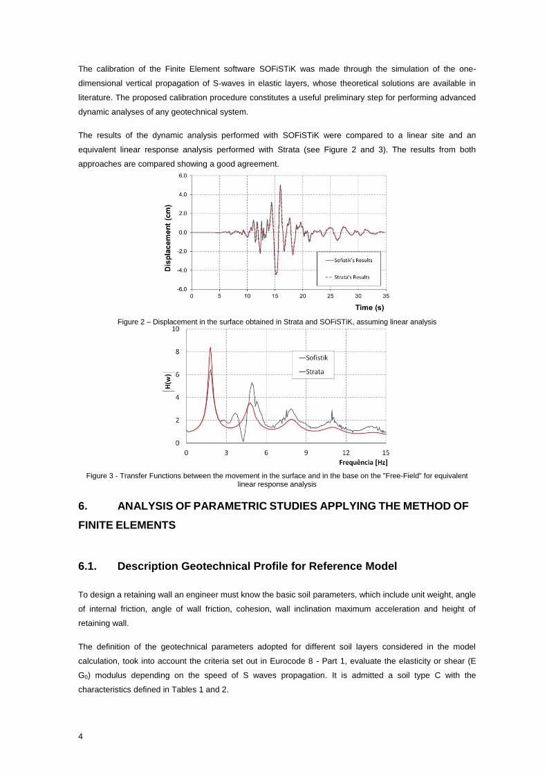
The results of the dynamic analysis performed with SOFiSTiK were compared to a linear site and an

equivalent linear response analysis performed with Strata (see Figure 2 and 3). The results from both

approaches are compared showing a good agreement.

Figure 2 – Displacement in the surface obtained in Strata and SOFiSTiK, assuming linear analysis

Figure 3 - Transfer Functions between the movement in the surface and in the base on the "Free-Field" for equivalent linear response analysis

6. ANALYSIS OF PARAMETRIC STUDIES APPLYING THE METHOD OF

FINITE ELEMENTS

6.1. Description Geotechnical Profile for Reference Model

To design a retaining wall an engineer must know the basic soil parameters, which include unit weight, angle

of internal friction, angle of wall friction, cohesion, wall inclination maximum acceleration and height of

retaining wall.

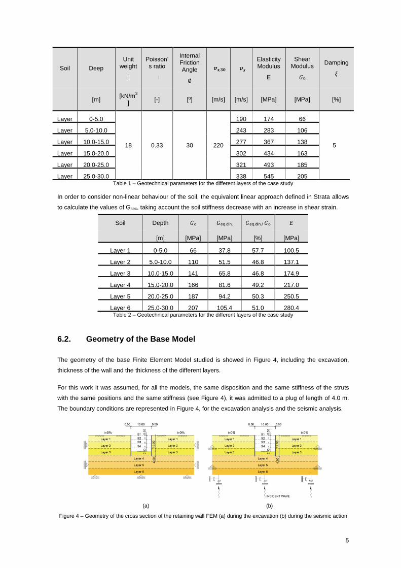
The definition of the geotechnical parameters adopted for different soil layers considered in the model

calculation, took into account the criteria set out in Eurocode 8 - Part 1, evaluate the elasticity or shear (E

G0) modulus depending on the speed of S waves propagation. It is admitted a soil type C with the

characteristics defined in Tables 1 and 2.

5

Soil Deep

Unit weight

Poisson’s ratio

Internal Friction Angle

∅

𝒗𝒔,𝟑𝟎 𝒗𝒔

Elasticity Modulus

E

Shear Modulus

𝐺0

Damping

𝜉

[m] [kN/m

3

] [-] [º] [m/s] [m/s] [MPa] [MPa] [%]

Layer 1

0-5.0

18 0.33 30 220

190 174 66

5

Layer 2

5.0-10.0 243 283 106

Layer 3

10.0-15.0 277 367 138

Layer 4

15.0-20.0 302 434 163

Layer 5

20.0-25.0 321 493 185

Layer 6

25.0-30.0 338 545 205 Table 1 – Geotechnical parameters for the different layers of the case study

In order to consider non-linear behaviour of the soil, the equivalent linear approach defined in Strata allows

to calculate the values of Gsec, taking account the soil stiffness decrease with an increase in shear strain.

Soil Depth 𝐺o 𝐺eq.din. 𝐺eq.din./ 𝐺o 𝐸

[m] [MPa] [MPa] [%] [MPa]

Layer 1 0-5.0 66 37.8 57.7 100.5

Layer 2 5.0-10.0 110 51.5 46.8 137.1

Layer 3 10.0-15.0 141 65.8 46.8 174.9

Layer 4 15.0-20.0 166 81.6 49.2 217.0

Layer 5 20.0-25.0 187 94.2 50.3 250.5

Layer 6 25.0-30.0 207 105.4 51.0 280.4 Table 2 – Geotechnical parameters for the different layers of the case study

6.2. Geometry of the Base Model

The geometry of the base Finite Element Model studied is showed in Figure 4, including the excavation,

thickness of the wall and the thickness of the different layers.

For this work it was assumed, for all the models, the same disposition and the same stiffness of the struts

with the same positions and the same stiffness (see Figure 4), it was admitted to a plug of length of 4.0 m.

The boundary conditions are represented in Figure 4, for the excavation analysis and the seismic analysis.

(a) (b)

Figure 4 – Geometry of the cross section of the retaining wall FEM (a) during the excavation (b) during the seismic action

6

6.3. Description of Seismic Action

The seismic action was defined based on the criteria defined in EC8 and the Portuguese National Annex,

considering that the case studies are located in the Lisbon area, i.e. the seismic zone 1.3 for Type 1 seismic

action, importance coefficient of type II, soil type C and 5% damping coefficient.

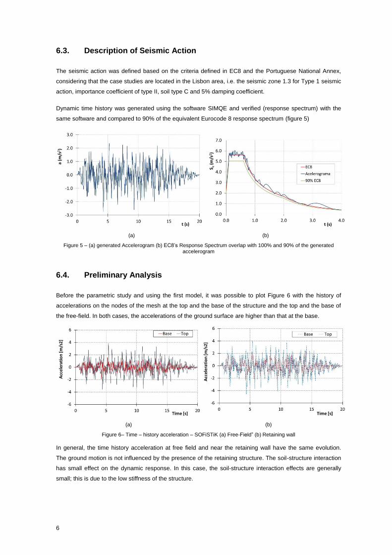
Dynamic time history was generated using the software SIMQE and verified (response spectrum) with the

same software and compared to 90% of the equivalent Eurocode 8 response spectrum (figure 5)

(a) (b)

Figure 5 – (a) generated Accelerogram (b) EC8’s Response Spectrum overlap with 100% and 90% of the generated accelerogram

6.4. Preliminary Analysis

Before the parametric study and using the first model, it was possible to plot Figure 6 with the history of

accelerations on the nodes of the mesh at the top and the base of the structure and the top and the base of

the free-field. In both cases, the accelerations of the ground surface are higher than that at the base.

(a) (b)

Figure 6– Time – history acceleration – SOFiSTiK (a) Free-Field” (b) Retaining wall

In general, the time history acceleration at free field and near the retaining wall have the same evolution.

The ground motion is not influenced by the presence of the retaining structure. The soil-structure interaction

has small effect on the dynamic response. In this case, the soil-structure interaction effects are generally

small; this is due to the low stiffness of the structure.

7

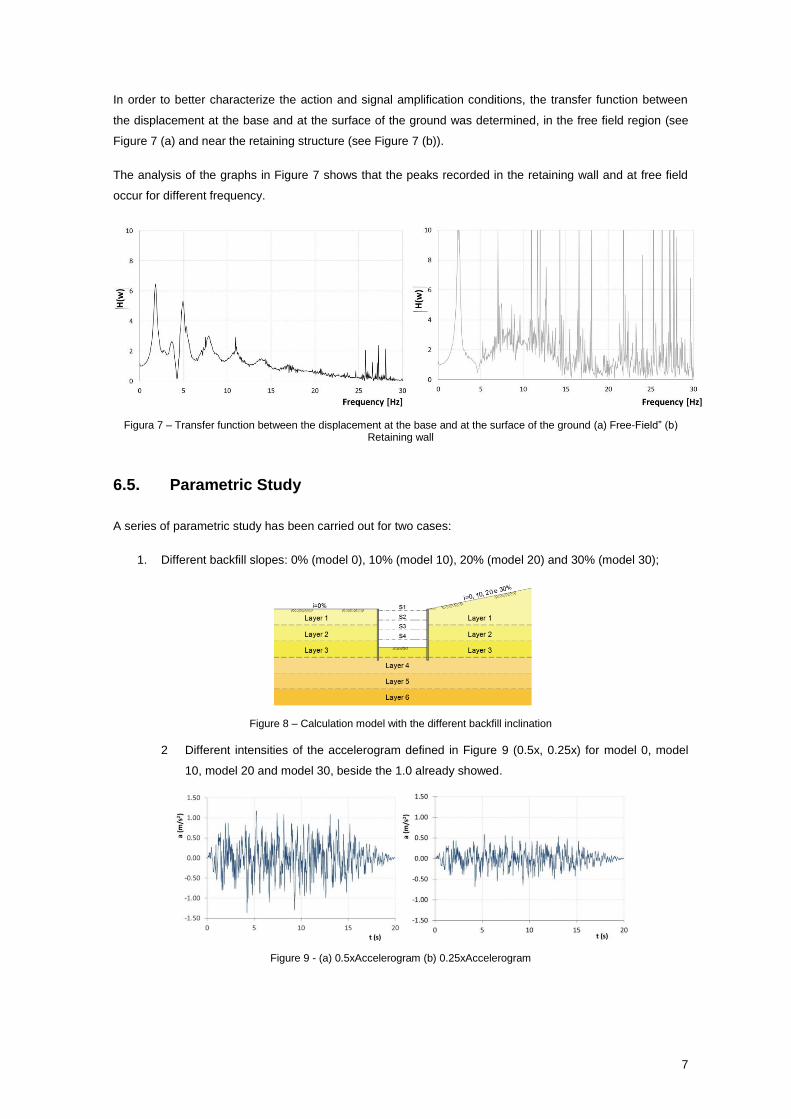
In order to better characterize the action and signal amplification conditions, the transfer function between

the displacement at the base and at the surface of the ground was determined, in the free field region (see

Figure 7 (a) and near the retaining structure (see Figure 7 (b)).

The analysis of the graphs in Figure 7 shows that the peaks recorded in the retaining wall and at free field

occur for different frequency.

Figura 7 – Transfer function between the displacement at the base and at the surface of the ground (a) Free-Field” (b) Retaining wall

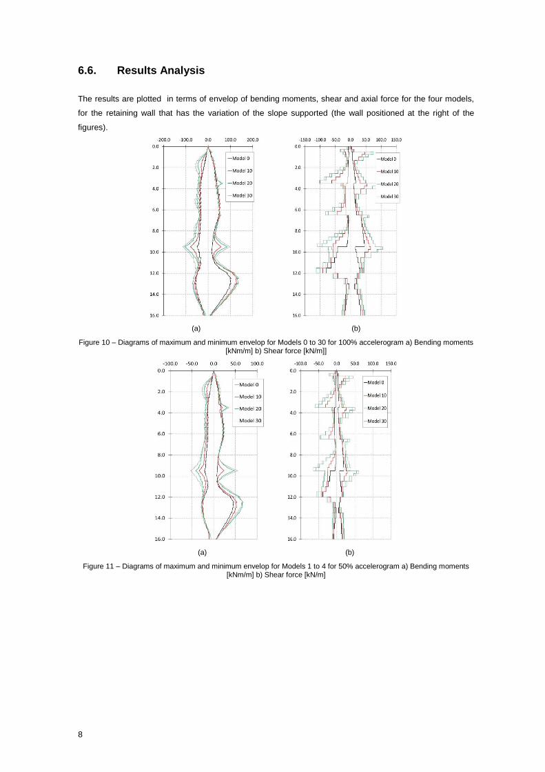
6.5. Parametric Study

A series of parametric study has been carried out for two cases:

1. Different backfill slopes: 0% (model 0), 10% (model 10), 20% (model 20) and 30% (model 30);

Figure 8 – Calculation model with the different backfill inclination

2 Different intensities of the accelerogram defined in Figure 9 (0.5x, 0.25x) for model 0, model

10, model 20 and model 30, beside the 1.0 already showed.

Figure 9 - (a) 0.5xAccelerogram (b) 0.25xAccelerogram

8

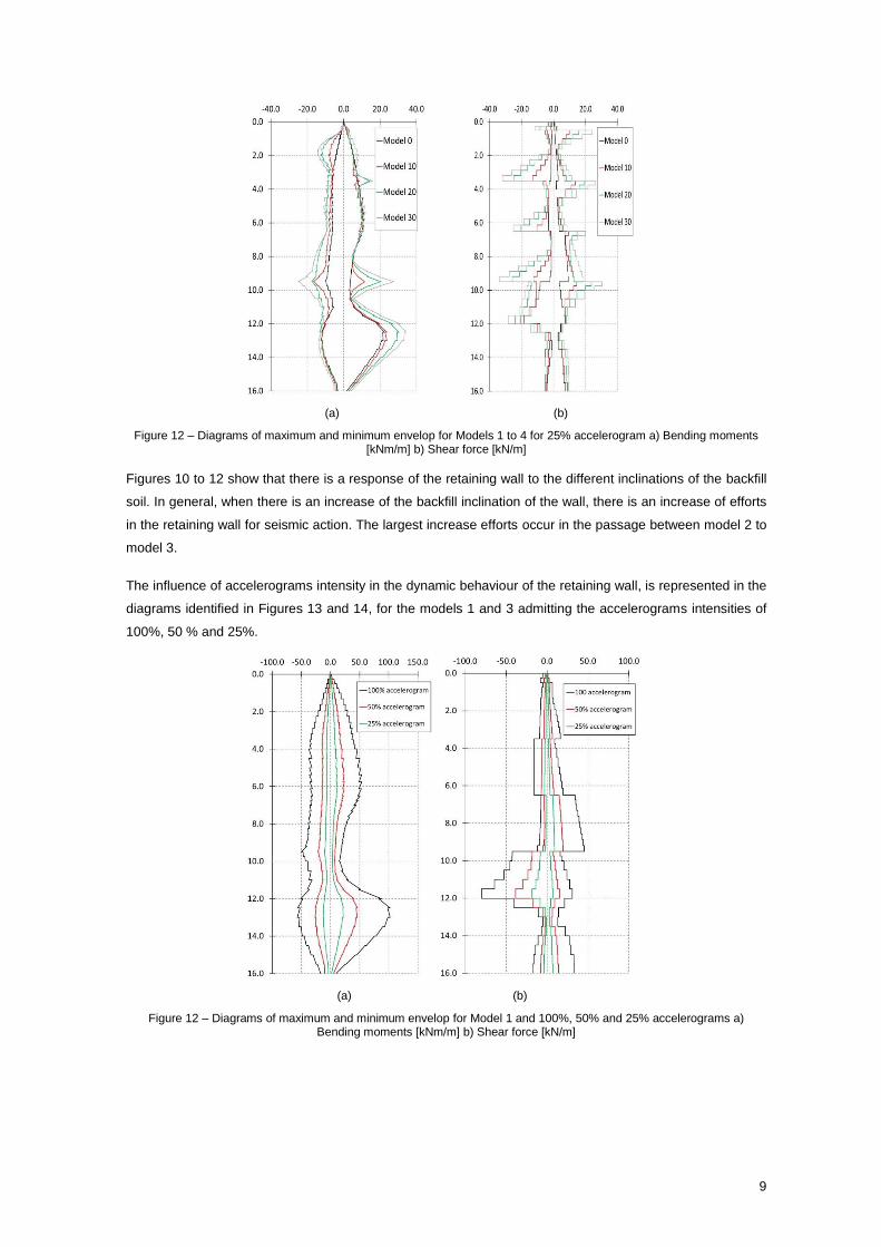
6.6. Results Analysis

The results are plotted in terms of envelop of bending moments, shear and axial force for the four models,

for the retaining wall that has the variation of the slope supported (the wall positioned at the right of the

figures).

(a) (b)

Figure 10 – Diagrams of maximum and minimum envelop for Models 0 to 30 for 100% accelerogram a) Bending moments [kNm/m] b) Shear force [kN/m]]

(a) (b)

Figure 11 – Diagrams of maximum and minimum envelop for Models 1 to 4 for 50% accelerogram a) Bending moments [kNm/m] b) Shear force [kN/m]

9

(a) (b)

Figure 12 – Diagrams of maximum and minimum envelop for Models 1 to 4 for 25% accelerogram a) Bending moments [kNm/m] b) Shear force [kN/m]

Figures 10 to 12 show that there is a response of the retaining wall to the different inclinations of the backfill

soil. In general, when there is an increase of the backfill inclination of the wall, there is an increase of efforts

in the retaining wall for seismic action. The largest increase efforts occur in the passage between model 2 to

model 3.

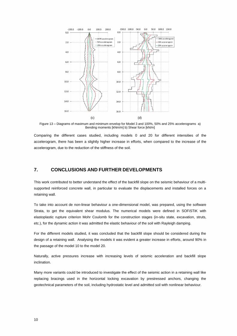
The influence of accelerograms intensity in the dynamic behaviour of the retaining wall, is represented in the

diagrams identified in Figures 13 and 14, for the models 1 and 3 admitting the accelerograms intensities of

100%, 50 % and 25%.

(a) (b)

Figure 12 – Diagrams of maximum and minimum envelop for Model 1 and 100%, 50% and 25% accelerograms a) Bending moments [kNm/m] b) Shear force [kN/m]

10

(c) (d)

Figure 13 – Diagrams of maximum and minimum envelop for Model 3 and 100%, 50% and 25% accelerograms a) Bending moments [kNm/m] b) Shear force [kN/m]

Comparing the different cases studied, including models 0 and 20 for different intensities of the

accelerogram, there has been a slightly higher increase in efforts, when compared to the increase of the

accelerogram, due to the reduction of the stiffness of the soil.

7. CONCLUSIONS AND FURTHER DEVELOPMENTS

This work contributed to better understand the effect of the backfill slope on the seismic behaviour of a multi-

supported reinforced concrete wall, in particular to evaluate the displacements and installed forces on a

retaining wall.

To take into account de non-linear behaviour a one-dimensional model, was prepared, using the software

Strata, to get the equivalent shear modulus. The numerical models were defined in SOFiSTiK with

elastoplastic rupture criterion Mohr Coulomb for the construction stages (in-situ state, excavation, struts,

etc.), for the dynamic action it was admitted the elastic behaviour of the soil with Rayleigh damping.

For the different models studied, it was concluded that the backfill slope should be considered during the

design of a retaining wall. Analysing the models it was evident a greater increase in efforts, around 90% in

the passage of the model 10 to the model 20.

Naturally, active pressures increase with increasing levels of seismic acceleration and backfill slope

inclination.

Many more variants could be introduced to investigate the effect of the seismic action in a retaining wall like

replacing bracings used in the horizontal locking excavation by prestressed anchors, changing the

geotechnical parameters of the soil, including hydrostatic level and admitted soil with nonlinear behaviour.