Download pdf - into two charmed mesons

Exclusive decays of �bJ and �b into two charmed mesons

Regina S. Azevedo,1,* Bingwei Long,1,2,† and Emanuele Mereghetti1,‡

1Department of Physics, University of Arizona, Tucson, Arizona 85721, USA2European Centre for Theoretical Studies in Nuclear Physics and Related Areas (ECT*), I-38100 Villazzano (TN), Italy

3Department of Physics, University of Arizona, Tucson, Arizona 85721, USA(Received 10 September 2009; published 23 October 2009)

We develop a framework to study the exclusive two-body decays of bottomonium into two charmed

mesons and apply it to study the decays of the C-even bottomonia. Using a sequence of effective field

theories, we take advantage of the separation between the scales contributing to the decay processes,

2mb � mc � �QCD. We prove that, at leading order in the EFT power counting, the decay rate factorizes

into the convolution of two perturbative matching coefficients and three nonperturbative matrix elements,

one for each hadron. We calculate the relations between the decay rate and nonperturbative bottomonium

and D-meson matrix elements at leading order, with next-to-leading log resummation. The phenomeno-

logical implications of these relations are discussed.

DOI: 10.1103/PhysRevD.80.074026 PACS numbers: 12.39.Hg, 13.25.Gv

I. INTRODUCTION

The exclusive two-body decays of heavy quarkoniuminto light hadrons have been studied in the framework ofperturbative QCD by many authors (for reviews, see [1,2]).These processes exhibit a large hierarchy between theheavy-quark mass, which sets the scale for annihilationprocesses, and the scales that determine the dynamicalstructure of the particles in the initial and final states.The large energy released in the annihilation of theheavy-quark–antiquark pair and the kinematics of the de-cay—with the products flying away from the decay point intwo back-to-back, almost lightlike directions—allow forrigorously deriving a factorization formula for the decayrate at leading twist (for an up-to-date review of the theo-retical and experimental status of the exclusive decays intolight hadrons, see [3]).

For the bottomonium system, a particularly interestingclass of two-body final states is the one containing twocharmed mesons. In these cases the picture is complicatedby the appearance of an additional intermediate scale, thecharm mass mc, which is much smaller than the bottommass mb but is large enough to be perturbative. Thesedecays differ significantly from those involving only lightquarks. The creation of mesons that are made up of purelylight quarks involves creating two quark-antiquark pairs,with the energy shared between the quark and antiquark ineach pair. In the production of two D mesons, however,almost all the energy of the bottomonium is carried awayby the heavy c and �c, while the light quark and antiquark,which bind to the �c and c, respectively, carry away(boosted) residual energies.

The existence of well-separated scales in the system andthe intuitive picture of the decay process suggest to tackle

the problem using a sequence of effective field theories(EFTs) that are obtained by subsequently integrating outthe dynamics relevant to the perturbative scalesmb andmc.In the first step, we integrate out the scalemb by describ-

ing the b and �b with nonrelativistic QCD (NRQCD) [4],and the highly energetic c and �c with two copies of soft-collinear effective theory (SCET) [5–9] in opposite light-cone directions. In the second step, we integrate out thedynamics manifested at scales of order mc by treating thequarkonium with potential NRQCD (pNRQCD) [10–12],and the D mesons with a boosted version of heavy-quarkeffective theory (HQET) [13–19]. The detailed explanationof why the aforementioned EFTs are employed is offeredin Sec. II. We will prove that, at leading order in the EFTexpansion, the decay rate factors into a convolution of twoperturbative matching coefficients and three (one for eachhadron) nonperturbative matrix elements. The nonpertur-bative matrix elements are process independent and encodeinformation on both the initial and final states.For simplicity, in this paper we focus on the decays of

the C-even quarkonia �bJ and �b that, at leading order inthe strong coupling �s, proceed via the emission of twovirtual gluons. The same method can be generalized to thedecays of C-odd states � and hb, which require an addi-tional virtual gluon. We also refrain from processes thathave vanishing contributions at leading order in the EFTpower counting. So the specific processes studied in thispaper are �b0;2 ! DD, �b0;2 ! D�D�, and �b ! DD� þc:c. However, the EFT approach developed in this paperenables one to systematically include power-suppressedeffects, making it possible to go beyond the leading-twistapproximation.The study of the inclusive and exclusive charm produc-

tion in bottomonium decays and the study of the roleplayed by the charm mass mc in such processes haverecently drawn renewed attention [20–23], in connectionwith the experimental advances spurred in the past fewyears by the abundance of bottomonium data produced at

*[email protected]†[email protected]‡[email protected]

PHYSICAL REVIEW D 80, 074026 (2009)

1550-7998=2009=80(7)=074026(23) 074026-1 � 2009 The American Physical Society

http://dx.doi.org/10.1103/PhysRevD.80.074026

facilities like BABAR, BELLE, and CLEO. The most no-table result was the observation of the bottomoniumground state �b, recently reported by the BABAR Col-laboration [24]. Furthermore, the CLEO Collaborationpublished the first results for several exclusive decays of�b into light hadrons [25] and for the inclusive decay of �b

into open charm [26]. In particular, they measured thebranching ratio Bð�bJ ! D0XÞ, where J is the total angu-lar momentum of the �b state, and conclusively showedthat for J ¼ 1 the production of open charm is substantial:Bð�b1ð1PÞ ! D0XÞ ¼ 12:59%� 1:94%. For the J ¼ 0, 2states the data are weaker, but the production of opencharm still appears to be relevant. The measurements ofthe CLEO Collaboration are in good agreement with theprediction of Bodwin et al. [20], where EFT techniques (inparticular, NRQCD) were, for the first time, applied tostudy the production of charm in bottomonium decays.

The double-charm decay channels analyzed here havenot yet been observed, so one of our aims is to see if theymay be observable given the current data. Unfortunately,the poor knowledge of the D-meson matrix elements pre-vents us from providing definitive predictions for the decayrates �ð�bJ ! DDÞ, �ð�bJ ! D�D�Þ, and �ð�b !DD� þ c:c:Þ. As we will show, these rates are indeedstrongly dependent on the parameters of the D- andD�-meson distribution amplitudes, in particular, on theirfirst inverse moments �D and �D� : the rates vary by anorder of magnitude in the accepted ranges for �D and �D� .On the other hand, the factorization formula implies thatthese channels, if measured with sufficient accuracy, couldconstrain the form of the D-meson distribution amplitudeand the value of its first inverse moment. In turn, the detailsof the D-meson structure are relevant to other D-mesonobservables, which are crucial for a model-independentdetermination of the Cabibbo-Kobayashi-Maskawa matrixelements jVcdj and jVcsj [27].

This paper is organized as follows. In Sec. II we discussthe degrees of freedom and the EFTs we use. In Sec. III Awe match QCD onto NRQCD and SCET at the scale 2mb.The renormalization-group equation (RGE) for the match-ing coefficient is derived and solved in Sec. III B. InSec. IVA the scale mc is integrated out by matchingNRQCD and SCET onto pNRQCD and boosted HQET(bHQET). The renormalization of the low-energy EFToperators is performed in Sec. IVB, with some technicaldetails left to Appendix A. The decay rates are calculatedin Sec. V using two model distribution amplitudes. InSec. VI we draw our conclusions.

II. DEGREES OF FREEDOM AND THEEFFECTIVE FIELD THEORIES

Several well-separated scales are involved in the decaysof the C-even bottomonia �b and �bJ into two D mesons,making them ideal processes for the application of EFTtechniques. The distinctive structures of the bottomonium

(a heavy-quark–antiquark pair) and the D meson (a boundstate of a heavy quark and a light quark) suggest that oneneeds different EFTs to describe the initial and final states.We first look at the initial state. The �b is the ground

state of the bottomonium system. It is a pseudoscalarparticle, with spin S ¼ 0, orbital angular momentum L ¼0, and total angular momentum J ¼ 0. In what follows wewill often use the spectroscopic notation 2Sþ1LJ, in whichthe �b is denoted by 1S0. The �bJ is a triplet of states with

quantum numbers 3PJ. The �b and �bJ are nonrelativisticbound states of a b quark and a �b antiquark. The scales inthe system are the b quark mass mb, the relative momen-tum of the b �b pair mbw, the binding energy mbw

2, and�QCD, the scale where QCD becomes strongly coupled. wis the relative velocity of the quark-antiquark pair in themeson, and from the bottomonium spectrum it can beinferred that w2 � 0:1. Since mb � �QCD, mb can be

integrated out in perturbation theory and the bottomoniumcan be described in NRQCD. The degrees of freedom ofNRQCD are nonrelativistic heavy quarks and antiquarks,with energy and momentum ðE; j ~pjÞ of order ðmbw

2; mbwÞ,light quarks and gluons. In NRQCD, the gluons can be softðmbw;mbwÞ, potential ðmbw

2; mbwÞ, and ultrasoft (usoft)ðmbw

2; mbw2Þ. The NRQCD Lagrangian is constructed as

a systematic expansion in 1=mb whose first few terms are

LNRQCD ¼ c y�iD0 þ

~D2

2mb

þ ~� � g ~B

2mb

þ . . .

�c

þ �y�iD0 �

~D2

2mb

� ~� � g ~B

2mb

þ . . .

��;

where c and �y annihilate a b quark and a �b antiquark,respectively, and � � � denotes higher-order contributions in1=mb. In NRQCD several mass scales are still dynamicaland different assumptions on the hierarchy of these scalesmay lead to different power countings for operators ofhigher dimensionality. However, as long as w � 1,higher-dimension operators are suppressed by powers ofw (for a critical discussion on the different power count-ings, we refer to [12]).NRQCD still contains interactions that can excite the

heavy quarkonium far from its mass shell, for example,through the interaction of a nonrelativistic quark with a softgluon. In the case mbw � �QCD, we can integrate out

these fluctuations, perturbatively matching NRQCD ontoa low-energy effective theory, pNRQCD. We are then leftwith a theory of nonrelativistic quarks and ultrasoft gluons,with nonlocal potentials induced by the integration oversoft- and potential-gluon modes. The interactions of theheavy quark with ultrasoft gluons are still described by theNRQCD Lagrangian, with the constraint that all the gluonsare ultrasoft. In the weak coupling regime mbw � �QCD,

the potentials are organized by an expansion in �sðmbwÞ,1=mb, and r, where r is the distance between the quark andantiquark in the quarkonium, r� 1=mbw. If we assume

AZEVEDO, LONG, AND MEREGHETTI PHYSICAL REVIEW D 80, 074026 (2009)

074026-2

mbw2 ��QCD, each term in the expansion has a definite

power counting in w and the leading potential isCoulombic, V � �sðmbwÞ=r.

An alternative approach, which does not require a two-step matching, has been developed in the effective theoryvelocity NRQCD (vNRQCD) [28–31]. In the vNRQCDapproach there is only one EFT below mb, which is ob-tained by integrating out all the off-shell fluctuations at thehard scale mb and introducing different fields for variouspropagating degrees of freedom (nonrelativistic quarks andsoft and ultrasoft gluons). In spite of the differences be-tween the two formalisms, pNRQCD and vNRQCD giveequivalent final answers in all the known examples inwhich both theories can be applied.

We now turn to the structure of the D meson. The mostrelevant features of theDmeson are captured by a descrip-tion in HQET. In HQET, in order to integrate out the inertscale mc, the momentum of the heavy quark is genericallywritten as [15]

p ¼ mcvþ k; (1)

where v is the four-velocity label, satisfying v2 ¼ 1, and kis the residual momentum. If one chooses v to be thecenter-of-mass velocity of the D meson, k scales as k�v�QCD. Introducing the light-cone vectors n

� ¼ ð1; 0; 0; 1Þand �n� ¼ ð1; 0; 0;�1Þ, one can express the residual mo-mentum in light-cone coordinates, k� ¼ �n � kn�=2þ n �k �n�=2þ k�? or simply k ¼ ðn � k; �n � k; ~k?Þ. There are tworelevant frames. One is theD-meson rest frame, in which vis conveniently chosen as v0 ¼ ð1; 0; 0; 0Þ, and the other isthe bottomonium rest frame, in which the D mesons arehighly boosted in opposite directions, with v chosen asv ¼ vD, the four-velocity of one of the D mesons. By asimple consideration of kinematics and the scaling k�v�QCD, one can work out the scalings for k in the two

frames. In the D-meson rest frame, k��QCDð1; 1; 1Þ, andin the bottomonium rest frame (supposing the D mesonmoving in the positive z direction),

k��QCDðn � vD; �n � vD; 1Þ ��QCD �n � vDð�2; 1; �Þ; (2)

where �n � vD � 2mb=mc and � ¼ mc=2mb � 1. It is con-venient for the calculation in this paper to use the botto-monium rest frame, so we drop the subscript in vD and weassume v ¼ vD in the rest of this paper. The momentumscaling in Eq. (2) is called ultracollinear (ucollinear), and

bHQET is the theory that describes heavy quarks withultracollinear residual momenta and light degrees of free-dom (including gluons and light quarks) with the samemomentum scaling.The bHQET Lagrangian is organized as a series in

powers of �QCD=mc and, for residual momentum ultracol-

linear in the n direction, the leading term is [18]

L bHQET ¼ �hniv �Dhn; (3)

where the field hn annihilates a heavy quark and thecovariant derivative D contains ultracollinear and ultrasoftgluons,

iD� ¼ n�

2ði �n � @þ g �n � AnÞ

þ �n�

2ðin � @þ gn � An þ gn � AusÞ

þ ði@�? þ gA�n;?Þ: (4)

The ultrasoft gluons only enter in the small component ofthe covariant derivative. This fact can be exploited todecouple ultrasoft and ultracollinear modes in theleading-order Lagrangian through a field redefinition remi-niscent of the collinear-ultrasoft decoupling in SCET[7,18]. The ultracollinear-ultrasoft decoupling is an essen-tial ingredient for the factorization of the decay rate.Therefore, the appropriate EFT to calculate the decay

rate is a combination of pNRQCD, for the bottomonium,and two copies of bHQET, with fields collinear to the n and�n directions, for theD and �Dmesons, symbolically writtenas EFTII � pNRQCDþ bHQET.As we mentioned earlier, we plan to describe the botto-

monium structure with a two-step scheme QCD !NRQCD ! pNRQCD. However, at the intermediate stage,where we first integrate out the hard scale 2mb and arrive atthe scale mbw, the D meson cannot yet be described inbHQET. This is because the interactions relevant at theintermediate scale mbw can change the c-quark velocityand leave the D meson off shell of order �ðmbwÞ2 �m2

c � �2QCD. Highly energetic c and �c traveling in oppo-

site directions can be described properly by SCET withmass. Thus, at the scale � ¼ 2mb, we match QCD onto anintermediate EFT, EFTI � NRQCDþ SCET, in which theEFT expansion is organized by � and w. The degrees offreedom of EFTI are tabulated in Table I.

TABLE I. Degrees of freedom in EFTIðNRQCDþ SCETÞ. w is the b �b relative velocity in the bottomonium rest frame, while ��mc=2mb is the SCET expansion parameter. We assume mbw�mc (or, equivalently, w� �) and mbw

2 �mb�2 ��QCD.

NRQCD Field Momentum SCET Field Momentum

Quark b, �b c b, � �b ðmbw2; mbwÞ c, �c �c

�n, ��cn 2mbð1; �2; �Þ, 2mbð�2; 1; �Þ

Gluon Potential A� ðmbw2; mbwÞ Collinear A

��n , A

�n 2mbð1; �2; �Þ, 2mbð�2; 1; �Þ

Soft A� ðmbw;mbwÞ Soft A�s 2mbð�; �; �Þ

Usoft A� ðmbw2; mbw

2Þ Usoft A�us 2mbð�2; �2; �2Þ

EXCLUSIVE DECAYS OF �bJ AND �b INTO . . . PHYSICAL REVIEW D 80, 074026 (2009)

074026-3

Then, we integrate out mc and mbw at the same time,matching EFTI onto EFTII at the scale �

0 ¼ mc. In EFTII,the low-energy approximation is organized by �QCD=mc

and w. The degrees of freedom of EFTII are summarized inTable II. When no subscript is specified in the rest of thispaper, any reference to EFT applies to both EFTI andEFTII. To facilitate the power counting, we adopt w� ��QCD=mc. As a first study, wewill perform in this paper the

leading-order calculation of the bottomonium decay rates.

III. NRQCDþ SCET

A. Matching

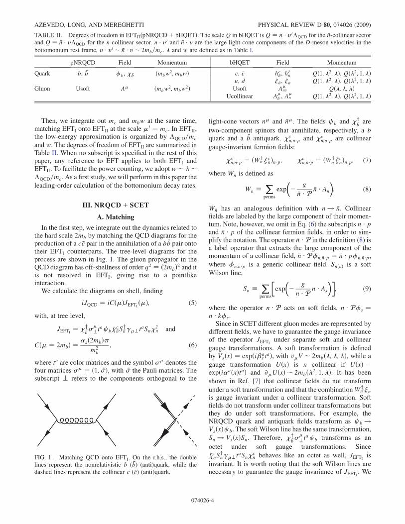
In the first step, we integrate out the dynamics related tothe hard scale 2mb by matching the QCD diagrams for theproduction of a c �c pair in the annihilation of a b �b pair ontotheir EFTI counterparts. The tree-level diagrams for theprocess are shown in Fig. 1. The gluon propagator in theQCD diagram has off-shellness of order q2 ¼ ð2mbÞ2 and itis not resolved in EFTI, giving rise to a pointlikeinteraction.

We calculate the diagrams on shell, finding

iJQCD ¼ iCð�ÞJEFTIð�Þ; (5)

with, at tree level,

JEFTI¼ �y

�b�

�?t

ac b ��c�nS

y�n��?taSn� �c

n and

Cð� ¼ 2mbÞ ¼ �sð2mbÞm2

b

; (6)

where ta are color matrices and the symbol �� denotes thefour matrices �� ¼ ð1; ~�Þ, with ~� the Pauli matrices. Thesubscript ? refers to the components orthogonal to the

light-cone vectors n� and �n�. The fields c b and �y�bare

two-component spinors that annihilate, respectively, a bquark and a �b antiquark. � �c

n; �n�p and �c�n;n�p are collinear

gauge-invariant fermion fields:

� �cn; �n�p � ðWy

n � �cnÞ �n�p; �c

�n;n�p � ðWy�n �

c�nÞn�p; (7)

where Wn is defined as

Wn � Xperms

exp

�� g

�n � P �n � An

�: (8)

W �n has an analogous definition with n ! �n. Collinearfields are labeled by the large component of their momen-tum. Note, however, we omit in Eq. (6) the subscripts n � pand �n � p of the collinear fermion fields, in order to sim-plify the notation. The operator �n � P in the definition (8) isa label operator that extracts the large component of themomentum of a collinear field, �n � Pn; �n�p ¼ �n � pn; �n�p,where n; �n�p is a generic collinear field. Snð �nÞ is a soft

Wilson line,

Sn � Xperms

�exp

�� g

n � P n � As

��; (9)

where the operator n � P acts on soft fields, n � Ps ¼n � ks.Since in SCET different gluon modes are represented by

different fields, we have to guarantee the gauge invarianceof the operator JEFTI

under separate soft and collinear

gauge transformations. A soft transformation is definedby VsðxÞ ¼ expði�a

s taÞ, with @�V � 2mbð�; �; �Þ, while a

gauge transformation UðxÞ is n collinear if UðxÞ ¼expði�aðxÞtaÞ and @�UðxÞ � 2mbð�2; 1; �Þ. It has been

shown in Ref. [7] that collinear fields do not transform

under a soft transformation and that the combinationWyn �n

is gauge invariant under a collinear transformation. Softfields do not transform under collinear transformations butthey do under soft transformations. For example, theNRQCD quark and antiquark fields transform as c b !VsðxÞc b. The soft Wilson line has the same transformation,

Sn ! VsðxÞSn. Therefore, �y�b��

?tac b transforms as an

octet under soft gauge transformations. Since

��c�nS

y�n��?taSn� �c

n behaves like an octet as well, JEFTIis

invariant. It is worth noting that the soft Wilson lines arenecessary to guarantee the gauge invariance of JEFTI

. We

TABLE II. Degrees of freedom in EFTIIðpNRQCDþ bHQETÞ. The scale Q in bHQET is Q ¼ n � v0�QCD for the �n-collinear sectorand Q ¼ �n � v�QCD for the n-collinear sector. n � v0 and �n � v are the large light-cone components of the D-meson velocities in the

bottomonium rest frame, n � v0 � �n � v� 2mb=mc. � and w are defined as in Table I.

pNRQCD Field Momentum bHQET Field Momentum

Quark b, �b c b, � �b ðmbw2; mbwÞ c, �c hc�n, h

�cn Qð1; �2; �Þ, Qð�2; 1; �Þ

u, d � �n, �n Qð1; �2; �Þ, Qð�2; 1; �ÞGluon Usoft A� ðmbw

2; mbw2Þ Usoft A

�us Qð�; �; �Þ

Ucollinear A��n , A

�n Qð1; �2; �Þ, Qð�2; 1; �Þ

FIG. 1. Matching QCD onto EFTI. On the r.h.s., the doublelines represent the nonrelativistic b ( �b) (anti)quark, while thedashed lines represent the collinear c ( �c) (anti)quark.


074026-4

have explicitly checked their appearance at one gluon bymatching QCD diagrams like the one in Fig. 1, with all thepossible attachments of an extra soft or collinear gluon,onto four-fermion operators in EFTI.

B. Running

The matching coefficient C and the effective operatorJEFTI

depend on the renormalization scale �. Since the

effective operator is sensitive to the low-energy scales inEFTI, logarithms that would appear in the evaluation ofJEFTI

are minimized by the choice ��mc. On the other

hand, since the coefficient encodes the high-energy dy-namics of the scale 2mb, such a choice would induce largelogarithms of mc=2mb in the matching coefficient. Theselogarithms can be resummed using RGEs in NRQCDþSCET.

The � dependence of JEFTIis governed by an equation

of the following form [32],

d

d ln�JEFTI

ð�Þ ¼ ��EFTIð�ÞJEFTI

ð�Þ; (10)

where the anomalous dimension �EFTIis given by

�EFTI¼ Z�1

EFTI

d

d ln�ZEFTI

(11)

and ZEFTIis the counterterm that relates the bare operator

Jð0ÞEFTIto the renormalized one, Jð0ÞEFTI

¼ ZEFTIð�ÞJEFTI

ð�Þ.Since the left-hand side (l.h.s.) of Eq. (5) is independent ofthe scale �, the RGE (10) can be recast as an equation forthe matching coefficient Cð�Þ,

d

d ln�Cð�Þ ¼ �EFTI

ð�ÞCð�Þ: (12)

The counterterm ZEFTIcancels the divergences that appear

in Green functions with the insertion of the operator JEFTI.

We calculate ZEFTIin the MS scheme by evaluating the

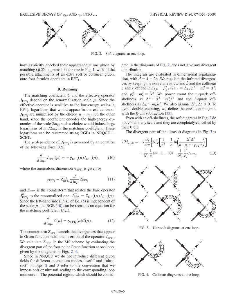
divergent part of the four-point Green function at one loop,given by the diagrams in Figs. 2–4.

Since in NRQCD we do not introduce different gluonfields for different momentum modes, ‘‘soft’’ and ‘‘ultra-soft’’ in Figs. 2 and 3 refer to the convention that weimpose soft or ultrasoft scaling to the corresponding loopmomentum. The potential region, which should be consid-

ered in the diagrams of Fig. 2, does not give any divergentcontribution.The integrals are evaluated in dimensional regulariza-

tion, with d ¼ 4� 2". We regulate the infrared divergen-ces by keeping the nonrelativistic b and �b and the collinearc and �c off shell: Eb; �b � ~p2

b; �b=2mb ¼ �b, p

2c �m2

c ¼ �2,

and p2�c �m2

c ¼ ��2. We power count the c-quark off-

shellness as �2 � ��2 �m2b�

2 and the b-quark off-

shellness as �b �mbw2. We also assume �2, ��2 > 0. To

avoid double counting, we define the one-loop integralswith the 0-bin subtraction [33].Even with an off-shellness, the soft diagrams in Fig. 2 do

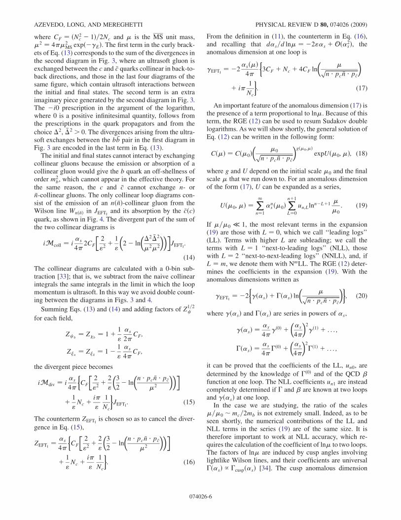
not contain any scale and they are completely cancelled bytheir 0 bin.The divergent part of the ultrasoft diagrams in Fig. 3 is

iMusoft ¼ �i�s

4

�2CF

�1

"2� 1

"ln

��2 ��2

n � pc �n � p �c�2

��

þ 1

Nc

1

"lnð�1� i0Þ � 1

Nc

1

"

�JEFTI

; (13)

FIG. 3. Ultrasoft diagrams at one loop.

FIG. 2. Soft diagrams at one loop.

FIG. 4. Collinear diagrams at one loop.


074026-5

where CF ¼ ðN2c � 1Þ=2Nc and � is the MS unit mass,

�2 ¼ 4�2MS expð��EÞ. The first term in the curly brack-

ets of Eq. (13) corresponds to the sum of the divergences inthe second diagram in Fig. 3, where an ultrasoft gluon isexchanged between the c and �c quarks collinear in back-to-back directions, and those in the last four diagrams of thesame figure, which contain ultrasoft interactions betweenthe initial and final states. The second term is an extraimaginary piece generated by the second diagram in Fig. 3.The �i0 prescription in the argument of the logarithm,where 0 is a positive infinitesimal quantity, follows fromthe prescriptions in the quark propagators and from the

choice �2, ��2 > 0. The divergences arising from the ultra-soft exchanges between the b �b pair in the first diagram inFig. 3 are encoded in the last term in Eq. (13).

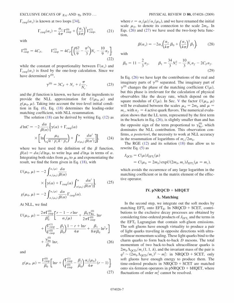
The initial and final states cannot interact by exchangingcollinear gluons because the emission or absorption of acollinear gluon would give the b quark an off-shellness oforder m2

b, which cannot appear in the effective theory. For

the same reason, the c and �c cannot exchange n- or�n-collinear gluons. The only collinear loop diagrams con-sist of the emission of an nð �nÞ-collinear gluon from theWilson line Wnð �nÞ in JEFTI

and its absorption by the �cðcÞquark, as shown in Fig. 4. The divergent part of the sum ofthe two collinear diagrams is

iMcoll ¼ i�s

42CF

�2

"2þ 1

"

�2� ln

��2 ��2

�2�2

��JEFTI

:

(14)

The collinear diagrams are calculated with a 0-bin sub-traction [33]; that is, we subtract from the naive collinearintegrals the same integrals in the limit in which the loopmomentum is ultrasoft. In this way we avoid double count-ing between the diagrams in Figs. 3 and 4.

Summing Eqs. (13) and (14) and adding factors of Z1=2c

for each field,

Zc b¼ Z�b

¼ 1þ 1

"

�s

2CF;

Z�n¼ Z� �n

¼ 1� 1

"

�s

4CF;

the divergent piece becomes

iMdiv ¼ i�s

4

�CF

�2

"2þ 2

"

�3

2� ln

�n � pc �n � p �c

�2

��

þ 1

"Nc þ i

"

1

Nc

�JEFTI

: (15)

The counterterm ZEFTIis chosen so as to cancel the diver-

gence in Eq. (15),

ZEFTI¼ �s

4

�CF

�2

"2þ 2

"

�3

2� ln

�n � pc �n � p �c

�2

��

þ 1

"Nc þ i

"

1

Nc

�: (16)

From the definition in (11), the counterterm in Eq. (16),and recalling that d�s=d ln� ¼ �2"�s þOð�2

sÞ, theanomalous dimension at one loop is

�EFTI¼ �2

�sð�Þ4

�3CF þ Nc þ 4CF ln

��ffiffiffiffiffiffiffiffiffiffiffiffiffiffiffiffiffiffiffiffiffiffiffiffi

n � pc �n � p �c

p�

þ i1

Nc

�: (17)

An important feature of the anomalous dimension (17) isthe presence of a term proportional to ln�. Because of thisterm, the RGE (12) can be used to resum Sudakov doublelogarithms. As wewill show shortly, the general solution ofEq. (12) can be written in the following form:

Cð�Þ ¼ Cð�0Þ�

�0ffiffiffiffiffiffiffiffiffiffiffiffiffiffiffiffiffiffiffiffiffiffiffiffin � pc �n � p �c

p�gð�0;�Þ

expUð�0; �Þ; (18)

where g and U depend on the initial scale �0 and the finalscale � that we run down to. For an anomalous dimensionof the form (17), U can be expanded as a series,

Uð�0; �Þ ¼ X1n¼1

�ns ð�0Þ

Xnþ1

L¼0

un;Llnn�Lþ1 �

�0

: (19)

If �=�0 � 1, the most relevant terms in the expansion(19) are those with L ¼ 0, which we call ‘‘leading logs’’(LL). Terms with higher L are subleading; we call theterms with L ¼ 1 ‘‘next-to-leading logs’’ (NLL), thosewith L ¼ 2 ‘‘next-to-next-leading logs’’ (NNLL), and, ifL ¼ m, we denote them with NmLL. The RGE (12) deter-mines the coefficients in the expansion (19). With theanomalous dimensions written as

�EFTI¼ �2

��ð�sÞ þ �ð�sÞ ln

��ffiffiffiffiffiffiffiffiffiffiffiffiffiffiffiffiffiffiffiffiffiffiffiffi

n � pc �n � p �c

p��; (20)

where �ð�sÞ and �ð�sÞ are series in powers of �s,

�ð�sÞ ¼ �s

4�ð0Þ þ

��s

4

�2�ð1Þ þ . . . ;

�ð�sÞ ¼ �s

4�ð0Þ þ

��s

4

�2�ð1Þ þ . . . ;

it can be proved that the coefficients of the LL, un0, are

determined by the knowledge of �ð0Þ and of the QCD �function at one loop. The NLL coefficients un1 are insteadcompletely determined if � and � are known at two loopsand �ð�sÞ at one loop.In the case we are studying, the ratio of the scales

�=�0 �mc=2mb is not extremely small. Indeed, as to beseen shortly, the numerical contributions of the LL andNLL terms in the series (19) are of the same size. It istherefore important to work at NLL accuracy, which re-quires the calculation of the coefficient of ln� to two loops.The factors of ln� are induced by cusp angles involvinglightlike Wilson lines, and their coefficients are universal�ð�sÞ / �cuspð�sÞ [34]. The cusp anomalous dimension


074026-6

�cuspð�sÞ is known at two loops [34],

�cuspð�sÞ ¼ �s

4�ð0Þcusp þ

��s

4

�2�ð1Þcusp; (21)

with

�ð0Þcusp ¼ 4CF; �ð1Þ

cusp ¼ 4CF

��67

9� 2

3

�Nc � 10

9nf

�;

(22)

while the constant of proportionality between �ð�sÞ and�cuspð�sÞ is fixed by the one-loop calculation. Since we

have determined �ð0Þ,

�ð0Þ ¼ 3CF þ Nc þ i

Nc

; (23)

and the � function is known, we have all the ingredients toprovide the NLL approximation for Uð�0; �Þ andgð�0; �Þ. Taking into account the tree-level initial condi-tion in Eq. (6), Eq. (18) determines the leading-ordermatching coefficient, with NLL resummation.

The solution (18) can be derived by writing Eq. (12) as

d lnC ¼ �2d�

�ð�Þ��ð�Þ þ �cuspð�Þ

�ln

��0ffiffiffiffiffiffiffiffiffiffiffiffiffiffiffiffiffiffiffiffiffiffiffiffi

n � pc �n � p �c

p�þ

Z �

�ð�0Þd�0

�ð�0Þ��; (24)

where we have used the definition of the � function,�ð�Þ ¼ d�=d ln�, to write ln� and d ln� in terms of �.Integrating both sides from�0 to� and exponentiating theresult, we find the form given in Eq. (18), with

Uð�0; �Þ ¼ �2Z �sð�Þ

�sð�0Þd�

�ð�Þ

��ð�Þ þ �cuspð�Þ

Z �

�ð�0Þd�0

�ð�0Þ�;

gð�0; �Þ ¼ �2Z �sð�Þ

�sð�0Þd�

�ð�Þ�cuspð�Þ:

(25)

At NLL, we find

Uð�b;�Þ ¼ 2�ð0Þcusp

�20

�r� 1� r lnr

�sð�Þ þ �0�ð0ÞRe

2�ð0Þcusp

lnr

þ��ð1Þcusp

�ð0Þcusp

� �1

�0

�1� rþ lnr

4þ �1

8�0

ln2r

�

þ �ð0ÞIm

�0

lnr; (26)

and

gð�b;�Þ ¼ �ð0Þcusp

�0

�lnrþ

��ð1Þcusp

�ð0Þcusp

� �1

�0

��sð�bÞ4

ðr� 1Þ�;

(27)

where r ¼ �sð�Þ=�sð�bÞ, and we have renamed the initialscale �b, to denote its connection to the scale 2mb. InEqs. (26) and (27) we have used the two-loop beta func-tion,

�ð�sÞ ¼ �2�s

��s

4�0 þ

��s

4

�2�1

�; (28)

with

�0 ¼ 11� 2

3nf; �1 ¼ 34

3N2

c � 10

3Ncnf � 2CFnf:

(29)

In Eq. (26) we have kept the contributions of the real and

imaginary parts of �ð0Þ separated. The imaginary part of

�ð0Þ changes the phase of the matching coefficient Cð�Þ,but this phase is irrelevant for the calculation of physicalobservables like the decay rate, which depend on thesquare modulus of Cð�Þ. In Sec. V the factor Uð�b;�Þwill be evaluated between the scales �b ¼ 2mb and � ¼mc, with nf ¼ 4 active quark flavors. The numerical evalu-

ation shows that the LL term, represented by the first termin the brackets in Eq. (26), is slightly smaller than and has

the opposite sign of the term proportional to �ð0ÞRe , which

dominates the NLL contribution. This observation con-firms, a posteriori, the necessity to work at NLL accuracyin the resummation of logarithms of mc=2mb.The RGE (12) and its solution (18) thus allow us to

rewrite Eq. (5) as

JQCD ¼ Cð�ÞJEFTIð�Þ

¼ Cð�b ¼ 2mbÞ expUð2mb;mcÞJEFTIð� ¼ mcÞ;

which avoids the occurrence of any large logarithm in thematching coefficient or in the matrix element of the effec-tive operator.

IV. pNRQCDþ bHQET

A. Matching

In the second step, we integrate out the soft modes bymatching EFTI onto EFTII. In NRQCDþ SCET, contri-butions to the exclusive decay processes are obtained byconsidering time-ordered products of JEFTI

and the terms in

the EFTI Lagrangian that contain soft-gluon emissions.The soft gluons have enough virtuality to produce a pairof light quarks traveling in opposite directions with ultra-collinear momentum scaling. These light quarks bind to thecharm quarks to form back-to-back D mesons. The totalmomentum of two back-to-back ultracollinear quarks is2mb�QCD=mcð1; 1; �Þ, and the invariant mass of the pair is

q2 � ð2mb�QCD=mcÞ2 �m2c: in NRQCDþ SCET, only

soft gluons have enough energy to produce them. Thetime-ordered products in NRQCDþ SCET are matchedonto six-fermion operators in pNRQCDþ bHQET, wherefluctuations of order m2

c cannot be resolved.


074026-7

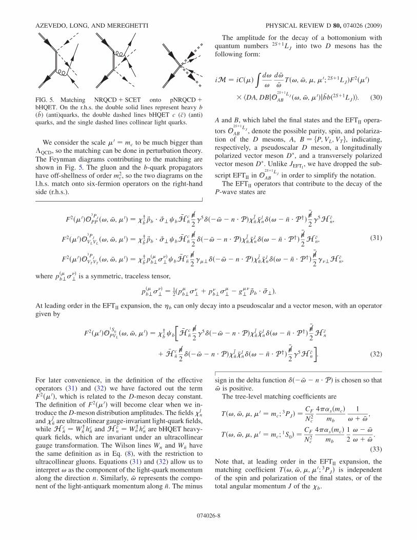
We consider the scale �0 ¼ mc to be much bigger than�QCD, so the matching can be done in perturbation theory.

The Feynman diagrams contributing to the matching areshown in Fig. 5. The gluon and the b-quark propagatorshave off-shellness of order m2

c, so the two diagrams on thel.h.s. match onto six-fermion operators on the right-handside (r.h.s.).

The amplitude for the decay of a bottomonium withquantum numbers 2Sþ1LJ into two D mesons has thefollowing form:

iM ¼ iCð�ÞZ d!

!

d �!

�!Tð!; �!;�;�0; 2Sþ1LJÞF2ð�0Þ

hDA;DBjO2Sþ1LJ

AB ð!; �!;�0Þj �bbð2Sþ1LJÞi: (30)

A and B, which label the final states and the EFTII opera-

tors O2Sþ1LJ

AB , denote the possible parity, spin, and polariza-tion of the D mesons, A, B ¼ fP; VL; VTg, indicating,respectively, a pseudoscalar D meson, a longitudinallypolarized vector meson D�, and a transversely polarizedvector meson D�. Unlike JEFTI

, we have dropped the sub-

script EFTII in O2Sþ1LJ

AB in order to simplify the notation.The EFTII operators that contribute to the decay of the

P-wave states are

F2ð�0ÞO3PJ

PP ð!; �!;�0Þ ¼ �y�b~pb � ~�?c b

�H c�n

6n2�5�ð� �!� n � P Þ��l

�n ��ln�ð!� �n � P yÞ

�6n2�5H �c

n;

F2ð�0ÞO3PJ

VLVLð!; �!;�0Þ ¼ �y

�b~pb � ~�?c b

�H c�n

6n2�ð� �!� n � P Þ��l

�n ��ln�ð!� �n � P yÞ

�6n2H �c

n;

F2ð�0ÞO3PJ

VTVTð!; �!;�0Þ ¼ �y

�bpð�b?�

Þ?c b

�H c�n

6n2��?�ð� �!� n � P Þ��l

�n ��ln�ð!� �n � P yÞ

�6n2� ?H �c

n;

(31)

where pð�b?�

Þ? is a symmetric, traceless tensor,

pð�b?�

Þ? ¼ 1

2ðp�b?�

? þ p

b?��? � g�

? ~pb � ~�?Þ:At leading order in the EFTII expansion, the �b can only decay into a pseudoscalar and a vector meson, with an operatorgiven by

F2ð�0ÞO1S0

PVLð!; �!;�0Þ ¼ �y

�bc b

��H c

�n

6n2�5�ð� �!� n � P Þ��l

�n ��ln�ð!� �n � P yÞ

�6n2H �c

n

þ �H c�n

6n2�ð� �!� n � P Þ��l

�n ��ln�ð!� �n � P yÞ

�6n2�5H �c

n

�: (32)

For later convenience, in the definition of the effectiveoperators (31) and (32) we have factored out the termF2ð�0Þ, which is related to the D-meson decay constant.The definition of F2ð�0Þ will become clear when we in-troduce theD-meson distribution amplitudes. The fields �l

n

and ��l�n are ultracollinear gauge-invariant light-quark fields,

while H c�n ¼ Wy

�n hc�n and H �c

n ¼ Wyn h �c

n are bHQET heavy-quark fields, which are invariant under an ultracollineargauge transformation. The Wilson lines Wn and W �n havethe same definition as in Eq. (8), with the restriction toultracollinear gluons. Equations (31) and (32) allow us tointerpret! as the component of the light-quark momentumalong the direction n. Similarly, �! represents the compo-nent of the light-antiquark momentum along �n. The minus

sign in the delta function �ð� �!� n � P Þ is chosen so that�! is positive.The tree-level matching coefficients are

Tð!; �!;�;�0 ¼ mc;3PJÞ ¼

CF

N2c

4�sðmcÞmb

1

!þ �!;

Tð!; �!;�;�0 ¼ mc;1S0Þ ¼

CF

N2c

4�sðmcÞmb

1

2

!� �!

!þ �!:

(33)

Note that, at leading order in the EFTII expansion, thematching coefficient Tð!; �!;�;�0; 3PJÞ is independentof the spin and polarization of the final states, or of thetotal angular momentum J of the �b.

FIG. 5. Matching NRQCDþ SCET onto pNRQCDþbHQET. On the r.h.s. the double solid lines represent heavy b( �b) (anti)quarks, the double dashed lines bHQET c ( �c) (anti)quarks, and the single dashed lines collinear light quarks.


074026-8

An important feature of bHQET is that the ultracollinearand ultrasoft sectors can be decoupled at leading order inthe power counting by a field redefinition reminiscent ofthe collinear-usoft decoupling in SCET [7,8]. For bHQETin the n direction, the decoupling is achieved by defining

h �cn ! Ynh

�cn and ��l

n ! ��lnY

yn , where Yn is an ultrasoft

Wilson line,

Yn ¼ Xperms

�exp

�� g

n � P n � Aus

��: (34)

An analogous redefinition with n ! �n decouples ultrasoftfrom �n-ultracollinear quarks and gluons. These redefini-tions do not affect the operators in Eqs. (31) and (32)because all the induced Wilson lines cancel out. As aconsequence, at leading order in the EFTII power counting,there is no interaction between the initial and the finalstates, since the former can only emit and absorb ultrasoftgluons that do not couple to ultracollinear degrees of free-dom. Furthermore, fields in the two copies of bHQET,boosted in opposite directions, cannot interact with eachother because the interaction with an �n-ultracollinear gluonwould give an n-ultracollinear quark or gluon a virtualityof order m2

c, which, however, cannot appear in EFTII. The

matrix elements of the operators O2Sþ1LJ

AB ð!; �!;�Þ, there-fore, factorize as

F2ð�0ÞhABjO2Sþ1LJ

AB ð!; �!;�0Þj �bbi

¼ h0j�y�bT

2Sþ1LJ

AB c bj �bbihAj �H c�n

6n2�A�ð� �!� n � P Þ

��l�nj0ihBj ��l

n�ð!� �n � P yÞ�6n2�BH �c

nj0i; (35)

where �A ¼ f�5; 1; ��?g and T

2Sþ1LJ

AB ¼ f1; ~pb �~�?; p

ð�b?�

Þ?g. The charge-conjugated contribution is

understood in the �b case.The quarkonium state and the D mesons in Eq. (35)

have, respectively, nonrelativistic and HQET normaliza-tion:

h�bJðE0; ~p0Þj�bJðE; ~pÞi ¼ ð2Þ3�ð3Þð ~p� ~p0Þ;hDðv0; k0ÞjDðv; kÞi ¼ 2v0�v;v0 ð2Þ3�ð3Þð ~k� ~k0Þ;

where v0 is the 0th component of the four-velocity v�.TheD-meson matrix elements can be expressed in terms

of the D-meson light-cone distribution amplitudes:

hPj ��ln

�6n2�5�ð!� �n � P yÞH �c

nj0i

¼ iFPð�0Þ �n � v2

Pð!;�0Þ;

hVLj ��ln

�6n2�ð!� �n � P yÞH �c

nj0i

¼ FVLð�0Þ �n � v

2VL

ð!;�0Þ;

hVTj ��ln

�6n2��?�ð!� �n � P yÞH �c

nj0i

¼ FVTð�0Þ �n � v

2"�?VT

ð!;�0Þ;

(36)

where "�? is the transverse polarization of the vector me-

son. The constants FAð�0Þ, with A ¼ fP; VL; VTg, are re-lated to the matrix elements of the local heavy-lightcurrents in coordinate space. In the heavy-quark limit,where D and D� are degenerate, FA is the same for allthe three states: F � FP ¼ FVL

¼ FVT. In this limit,

h0j ��ln

�6n2�5hcnð0ÞjPi ¼ �iFð�0Þ �n � v0

2: (39)

At tree level, the matrix element is proportional to theD-meson decay constant fD ¼ 205:8� 8:5� 2:5 MeV[35]. More precisely, Fð�0Þ ¼ fD

ffiffiffiffiffiffiffimD

p, where the factorffiffiffiffiffiffiffi

mDp

is due to HQET normalization. The scale dependence

of F is determined by the renormalization of heavy-lightHQET currents. At one loop, Ref. [32] showed that

d

d ln�0 Fð�0Þ ¼ ��FFð�0Þ ¼ 3CF

�s

4Fð�0Þ: (40)

The pNRQCD matrix elements can be expressed interms of the heavy quarkonium wave functions. The op-

erator �y�b~pb � ~�?c b contains a component with J ¼ 0 and

a component with J ¼ 2 and Jz ¼ 0, so its matrix elementhas nonvanishing overlap with both �b0 and �b2. The

operator �y�bpð�b � Þ

?c b instead has only contributions with

J ¼ 2 and Jz ¼ �2, and therefore it only overlaps with�b2. In terms of the bottomonium wave functions, thepNRQCD matrix elements are expressed as

h0j�y�b~pb � ~�?c bj�b0i ¼ 2ffiffiffi

3p

ffiffiffiffiffiffiffiffiffi3Nc

2

sR0�b0

ð0; �0Þ; (41)

h0j�y�b~pb � ~�?c bj�b2i ¼ �

ffiffiffiffiffiffi2

15

s ffiffiffiffiffiffiffiffiffi3Nc

2

sR0�b2

ð0; �0Þ; (42)

h0j�y�bpð�b � Þ

?c bj�b2i ¼ ð"ð2Þ� þ "ð�2Þ� Þ

ffiffiffiffiffiffiffiffiffi3Nc

2

sR0�b2

ð0; �0Þ;(43)

where R0�bJ

ð0Þ is the derivative of the radial wave function


074026-9

of the �bJ evaluated at the origin. At leading order, thepNRQCD Hamiltonian does not depend on J, so, up tocorrections of order w2, R0

�b2ð0Þ ¼ R0

�b0ð0Þ. The numerical

prefactors in Eqs. (41) and (42) follow from decomposing

~pb � ~�? into components with definite Jz. "ðjÞ� is the po-

larization tensor of the �b2 state, and Eq. (53) states that, atleading order in the w2 expansion, only the particles withpolarization Jz ¼ �2 contribute to �b2 decay into twotransversely polarized vector mesons. Similarly, one finds

h0j�y�bc bj�bi ¼

ffiffiffiffiffiffiffiNc

2

sR�b

ð0; �0Þ: (44)

The factorization of the matrix elements (35) impliesthat the decay rate also factorizes. For the decays of �b0

and �b2 into two pseudoscalar mesons or two longitudi-nally polarized vector mesons, we find

�ð�b0 ! AAÞ ¼ 4

3

m2D

ffiffiffiffiffiffiffiffiffiffiffiffiffiffiffiffiffiffiffiffiffiffiffiffiffiffim2

�b0� 4m2

D

q8m�b0

3Nc

2jCð�Þj2jR0

�b0ð0; �0Þj2

�F2ð�0Þ n � v0

2

�n � v2

Z d!

!

d �!

�!Tð!; �!;�;�0; 3PJÞAð �!;�0ÞAð!;�0Þ

�2

(45)

and

�ð�b2 ! AAÞ ¼ 2

15

m2D


�b2� 4m2

D

q8m�b2

3Nc

2jCð�Þj2jR0

�b2ð0; �0Þj2

�F2ð�0Þn � v0

2

�n � v2

Z d!

!

d �!

�!Tð!; �!;�;�0; 3PJÞAð �!;�0ÞAð!;�0Þ

�2; (46)

where A ¼ P, VL. For the decay of �b2 into two transversely polarized vector mesons, one finds the decay rate by summingover the possible transverse polarizations:

�ð�b2 ! VTVTÞ ¼ 2

5

m2D


�b2� 4m2

D

q8m�b2

3Nc

2jCð�Þj2jR0

�b2ð0; �0Þj2

�F2ð�0Þ n � v0

2

�n � v2

Z d!

!

d �!

�!Tð!; �!;�;�0; 3PJÞVT

ð �!;�0ÞVTð!;�0Þ

�2: (47)

In the case of �b decay into a pseudoscalar and a longitudinally polarized vector meson, we find

�ð�b ! PVL þ c:c:Þ ¼m2

D

ffiffiffiffiffiffiffiffiffiffiffiffiffiffiffiffiffiffiffiffiffiffiffiffiffim2

�b� 4m2

D

q8m�b

Nc

2jCð�Þj2jR�b

ð0; �0Þj2 12

�F2ð�0Þn � v0

2

�n � v2

Z d!

!

d �!

�!Tð!; �!;�;�0; 1S0Þ

ðVLð �!;�0ÞPð!;�0Þ �VL

ð!;�0ÞPð �!;�0ÞÞ�2: (48)

Note that we are working in the limit mc ! 1, where themD� �mD mass splitting vanishes.

The factorized formulas Eqs. (35) and (45)–(48) are themain results of this paper. Each decay rate of (45)–(48)depends on two calculable matching coefficients, C and T,and three nonperturbative, process-independent matrix el-ements, namely, two D-meson distribution amplitudes andthe bottomonium wave function. In Sec. V we will providea model-dependent estimate of the decay rates (45)–(48)and will discuss the phenomenological implications. Weconclude this section by observing that all the nonpertur-bative matrix elements cancel out in the ratios �ð�b0 !PPÞ=�ð�b2 ! PPÞ and �ð�b0 ! VLVLÞ=�ð�b2 ! VLVLÞ,

since the spin symmetry of pNRQCD guaranteesR0�b0

ð0Þ ¼ R0�b2

ð0Þ, at leading order in EFTII. Neglecting

the �b0-�b2 mass difference, we find, up to corrections oforder w2,

�ð�b0 ! AAÞ=�ð�b2 ! AAÞ ¼ 4

3

15

2¼ 10; (49)

with A ¼ P, VL.

B. Running

The dependence of the matching coefficientTð!; �!;�;�0; 2Sþ1LJÞ and of the operators in Eqs. (45)–


074026-10

(48) on the scale�0 is driven by a RGE that can be obtainedby renormalizing the EFTII operators. The RGE for theEFTII operators, which also defines the anomalous dimen-sion �EFTII

, is similar to Eq. (10),

d

d ln�0 ½F2ð�0ÞO2Sþ1LJ

AB ð!; �!;�0Þ

¼ �Z

d!0 Z d �!0�EFTIIð!;!0; �!; �!0;�0ÞF2ð�0Þ

O2Sþ1LJ

AB ð!0; �!0; �0Þ: (50)

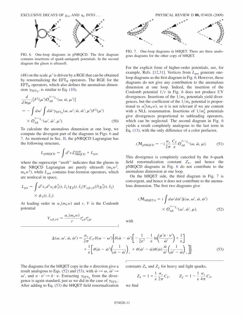
To calculate the anomalous dimension at one loop, wecompute the divergent part of the diagrams in Figs. 6 and7. As mentioned in Sec. II, the pNRQCD Lagrangian hasthe following structure,

LpNRQCD ¼Z

d3xLusoftNRQCD þ Lpot;

where the superscript ‘‘usoft’’ indicates that the gluons inthe NRQCD Lagrangian are purely ultrasoft ðmbw

2;mbw

2Þ, while Lpot contains four-fermion operators, which

are nonlocal in space,

Lpot ¼Z

d3x1d3x2c

y�ðt; ~x1Þ��ðt; ~x2ÞV��;��ð~rÞ�y

�ðt; ~x2Þ c �ðt; ~x1Þ:

At leading order in �sðmbwÞ and r, V is the Coulombpotential

V��;�� ¼ �sðmbwÞr

ta��ta��:

For the explicit form of higher-order potentials, see, forexample, Refs. [12,31]. Vertices from Lpot generate one-

loop diagrams as the first diagram in Fig. 6. However, thesediagrams do not give any contribution to the anomalousdimension at one loop. Indeed, the insertion of theCoulomb potential 1=r in Fig. 6 does not produce UVdivergences. Insertions of the 1=mb potentials yield diver-gences, but the coefficient of the 1=mb potential is propor-tional to �2

sðmbwÞ, so it is not relevant if we are contentwith a NLL resummation. Insertions of 1=m2

b potentials

give divergences proportional to subleading operators,which can be neglected. The second diagram in Fig. 6yields a result completely analogous to the last term inEq. (13), with the only difference of a color prefactor,

iMpNRQCD ¼ �i�s

2

CF

"O

2Sþ1LJ

AB ð!; �!;�Þ: (51)

This divergence is completely canceled by the b-quarkfield renormalization constant Zb, and hence thepNRQCD diagrams in Fig. 6 do not contribute to theanomalous dimension at one loop.On the bHQET side, the third diagram in Fig. 7 is

convergent, and hence it does not contribute to the anoma-lous dimension. The first two diagrams give

iMbHQET;�n ¼ iZ

d!0d �!0�ð!;!0; �!; �!0Þ

O2Sþ1LJ

AB ð!0; �!0; �Þ; (52)

with

�ð!;!0; �!; �!0Þ ¼ �s

2CF�ð!�!0Þ

��ð �!� �!0Þ

�� 1

2"2� 1

"ln

��0n � v0

�!0

�þ 1

"

�

þ 1

"

��ð �!� �!0Þ

�1

�!� �!0

�þþ �ð �!0 � �!Þ�ð �!Þ �!

�!0

�1

�!0 � �!

�þ

��: (53)

The diagrams for the bHQET copy in the n direction give aresult analogous to Eqs. (52) and (53), with �! ! !, �!0 !!0, and n � v0 ! �n � v. Extracting �EFTII

from the diver-gence is again standard, just as we did in the case of �EFTI

.After adding to Eq. (53) the bHQET field renormalization

constants Zh and Z� for heavy and light quarks,

Zh ¼ 1þ 1

"

�s

2CF; Z� ¼ 1� 1

"

�s

4CF;

we find

FIG. 6. One-loop diagrams in pNRQCD. The first diagramcontains insertions of quark-antiquark potentials. In the seconddiagram the gluon is ultrasoft.

FIG. 7. One-loop diagrams in bHQET. There are three analo-gous diagrams for the other copy of bHQET.


074026-11

�EFTIIð!;!0; �!; �!0;�0Þ ¼ 2�F�ð!�!0Þ�ð �!� �!0Þ þ �Oð!;!0; �!; �!0;�0Þ; (54)

with

�Oð!;!0; �!; �!0;�0Þ ¼ �s

44CF�ð!�!0Þ�ð �!� �!0Þ

��1þ ln

��0n � v0

�!0

�þ ln

��0 �n � v!0

��

� �s

44CF�ð!�!0Þ

��ð �!� �!0Þ

�1

�!� �!0

�þþ �ð �!0 � �!Þ�ð �!Þ �!

�!0

�1

�!0 � �!

�þ

�

� �s

44CF�ð �!� �!0Þ

��ð!�!0Þ

�1

!�!0

�þþ �ð!0 �!Þ�ð!Þ !

!0

�1

!0 �!

�þ

�: (55)

The term proportional to �F in Eq. (54) reproduces therunning of F2ð�0Þ (40). �O is responsible for the running oftheD-meson distribution amplitudes, and it agrees with theresult found in Ref. [36]. Also, in Eq. (36) the coefficient ofln�0 is proportional to �cuspð�sÞ. Note that, since thebHQET Lagrangian is spin independent, the anomalousdimension does not depend on the spin or on the polariza-tion of theDmeson in the final state, at leading order in thepower counting.

Using Eqs. (50) and (54) we find the following integro-differential RGE for the operator Oð!; �!;�0Þ:

d

d ln�0 Oð!; �!;�0Þ ¼ �Z

d!0 Z d �!0�Oð!;!0; �!; �!0;�0ÞOð!0; �!0; �0Þ; (56)

where we have dropped both the subscripts A, B, and thesuperscript 2Sþ1LJ does not depend on the quantum num-bers of the initial or final state. Using the fact that theconvolution of F2ð�0ÞTð!; �!;�;�0; 2Sþ1LJÞ and the op-

eratorO2Sþ1LJ

AB ð!; �!;�0Þ is�0 independent, we can write anequation for the coefficient,

d

d ln�0 ½F2ð�0ÞTð!; �!;�;�0Þ

¼Z

d!0 Z d �!0 !!0

�!

�!0 F2ð�0ÞTð!0; �!0; �;�0Þ

�Oð!0; !; �!0; �!;�0Þ¼

Zd!0 Z d �!0F2ð�0ÞTð!0; �!0; �;�0Þ

�Oð!;!0; �!; �!0;�0Þ; (57)

where the last step follows from the property of �O at oneloop,

!

!0�!

�!0 �Oð!0; !; �!0; �!;�0Þ ¼ �Oð!;!0; �!; �!0;�0Þ;

as can be explicitly verified from the expression inEq. (55).

Equation (57) can be solved following the methodsdescribed in Ref. [36]. We discuss the details of the solu-tion in Appendix A, where we derive the analytic expres-sions for Tð!; �!;�;�0; 3PJÞ and Tð!; �!;�;�0; 1S0Þ, with

the initial conditions at the scale �0c ¼ mc expressed in

Eq. (39).

V. DECAY RATES AND PHENOMENOLOGY

In Sec. IVA we gave the factorized expressions for thedecay rates (45)–(48): �ð�b0;2 ! PPÞ, �ð�b0;2 ! VLVLÞ,�ð�b2 ! VTVTÞ, and �ð�b ! PVL þ c:c:Þ. In Secs. III Band IVB we exploited the RGEs (12) and (57) to run thescales � and �0, respectively, from the matching scales� ¼ 2mb and�

0 ¼ mc to the natural scales that contributeto the matrix elements, � ¼ mc and �0 � 1 GeV, resum-ming in this way Sudakov logarithms of the ratiosmc=2mb

and mc=1 GeV.We proceed now to estimate the decay rates (45)–(48).

In order to do so, we need to evaluate the followingingredients: the light-cone distribution amplitudes of theD meson and of the longitudinally and transversely polar-ized D� mesons, and the wave functions of the states �b

and �bJ. In principle, these nonperturbative objects couldbe extracted from other �b, �b, and D-meson observables.In the case of the �b, the value of the wave function at theorigin can be obtained from a measurement of the inclusivehadronic width or of the decay rate for the electromagneticprocess �b ! ��, since they are both proportional tojR�b

ð0Þj2. Unfortunately, at the moment there are not suf-

ficient data on �b decays. Another way to proceed is to usethe spin symmetry of the leading-order pNRQCD Hamil-tonian, which implies R�b

ð0Þ ¼ R�ð0Þ, and to extract the

Upsilon wave function from �ð� ! eþe�Þ ¼ 1:28�0:07 KeV [37]. Using the leading-order expression for�ð� ! eþe�Þ [38], one finds jR�ð0Þj2 ¼ 6:92�0:38 GeV3, where the error only includes the experimentaluncertainty. The above value is in good agreement with thelattice evaluation by Bodwin, Sinclair, and Kim [39], and itfalls within the range of values obtained with four differentpotential models, as listed in Ref. [40].jR0

�b0;2ð0Þj2 can be obtained from the electromagnetic

decay �b0;2 ! ��. Unfortunately, such decay rates have

not been measured yet. The values listed in Ref. [40] rangefrom a minimum of jR0

�bJð0Þj2 ¼ 1:417 GeV5, obtained

with the Buchmuller-Tye potential [41], to a maximumof jR0

�bJð0Þj2 ¼ 2:067 GeV5, obtained with a Coulomb-

plus-linear potential. The lattice value is roughly of the


074026-12

same size, jR0�bJ

ð0Þj2 ¼ 2:3 GeV5, with an uncertainty of

about 15% [39]. We use this value in our estimate.For the pseudoscalar D-meson distribution amplitude,

we use two model functions widely adopted in the study ofB physics. A first possible choice, suggested, for example,in Ref. [36], is a simple exponential decay:

ExpP;0 ð!;�0 ¼ 1 GeVÞ ¼ �ð!Þ !

�2D

exp

�� !

�D

�: (58)

Another form, suggested in Ref. [42], is

BraunP;0 ð!;�0 ¼ 1 GeVÞ

¼ �ð ~!Þ 4

�D

~!

1þ ~!2

�1

1þ ~!2� 2ð�D � 1Þ

2ln ~!

�; (59)

where ~! ¼ !=�0. The theta function in Eqs. (58) and (59)reflects the fact that the distribution amplitudes Að!;�0Þ,with A ¼ fP; VL; VTg, have support on !> 0 [43].

The subscript 0 indicates that these functional forms arevalid in the D-meson rest frame, with a HQET velocitylabel v0 ¼ ð1; 0; 0; 0Þ. With the definition we adopt inEq. (36), the distribution amplitude is not boost invariant,and in the bottomonium rest frame, in which the D mesonhas a velocity ðn � v; �n � v; 0Þ � ðmc=2mb; 2mb=mc; 0Þ, itbecomes

Pð!;�0Þ ¼ 1

�n � vP;0

�!

�n � v ;�0�; (60)

as shown in Appendix B. �D and �D in Eqs. (58) and (59)are, respectively, the first inverse moment and the firstlogarithmic moment of the D-meson distribution ampli-tude in the D-meson rest frame,

��1D ð�0Þ ¼

Z 1

0

d!

!P;0ð!;�0Þ;

�Dð�0Þ��1D ð�0Þ ¼ �

Z 1

0

d!

!ln

�!

�0

�P;0ð!;�0Þ:

Furthermore, we assume that the vector-meson distributionamplitudes VL

ð!Þ and VTð!Þ have the same functional

form asPð!Þ, but with different parameters �D�L,�D�

Land

�D�T, �D�

T.

The D-meson distribution amplitude and its momentshave not been intensively studied unlike, for example, theB-meson distribution amplitude. Therefore, we invokeheavy-quark symmetry and use the moments of theB-meson distribution amplitude in order to estimate thedecay rate. However, the value of �B is affected by anoticeable uncertainty. Using QCD sum rules, Braunet al. estimated [42] �Bð�0 ¼ 1 GeVÞ ¼ 0:460�0:110 GeV, where the uncertainty is about 25%. Otherauthors [44–46] give slightly different central values andcomparable uncertainties, so that �B falls in the range0:350 GeV< �B < 0:600 GeV. The first logarithmic mo-ment �D is given in Ref. [42], �D ¼ �Bð�0 ¼ 1 GeVÞ ¼1:4� 0:4. We assume that the moments of the D�-meson

distribution amplitudes fall in the same range as the mo-ments of Pð!Þ.We evaluate numerically the convolution integrals in

Eqs. (45)–(48). We choose the matching scales �b and�0

c to be 2mb andmc, respectively. Using the RGEs we runthe matching coefficients down to the scales � ¼ mc and�0 ¼ 1 GeV. For the b and c quark masses we adopt the 1Smass definition [47],

mbð1SÞ ¼ m�

2¼ 4730:15� 0:13 MeV;

mcð1SÞ ¼mJ=c

2¼ 1548:46� 0:01 MeV:

(61)

The values of �s at the relevant scales are [37] �sð2mbÞ ¼0:178� 0:005, �sðmcÞ ¼ 0:340� 0:020, and�sð1 GeVÞ � 0:5. With these choices, the value of g inEq. (A5) is gðmc; 1 GeVÞ ¼ �0:12� 0:02.The decay rates �ð�bJ ! AAÞ with A ¼ fP; VL; VTg,

(45)–(47), depend on the masses of the �bJ and of the Dmesons, whose most recent values are reported inRef. [37]. Since the effects due to the mass splitting ofthe �bJ and D multiplets are subleading in the EFT powercounting, we use in the evaluation the average mass of the�bJ multiplet and the average mass of D and D� mesons:m�bJ

¼ 9898:87� 0:28� 0:31 MeV and mD ¼1973:27� 0:18 MeV. Therefore, the velocity of the Dmesons in �bJ decay is �n � v ¼ n � v0 ¼ m�bJ

=mD ¼5:02, with negligible error. The decay rate �ð�b ! PVL þc:c:Þ (48) depends on the mass of the �b, which has beenrecently measured: m�b

¼ 9388:9þ3:1�2:3 � 2:7 MeV [24].

The velocity of the D meson in the �b decay is �n � v ¼n � v0 ¼ m�b

=mD ¼ 4:76, again with negligible error.

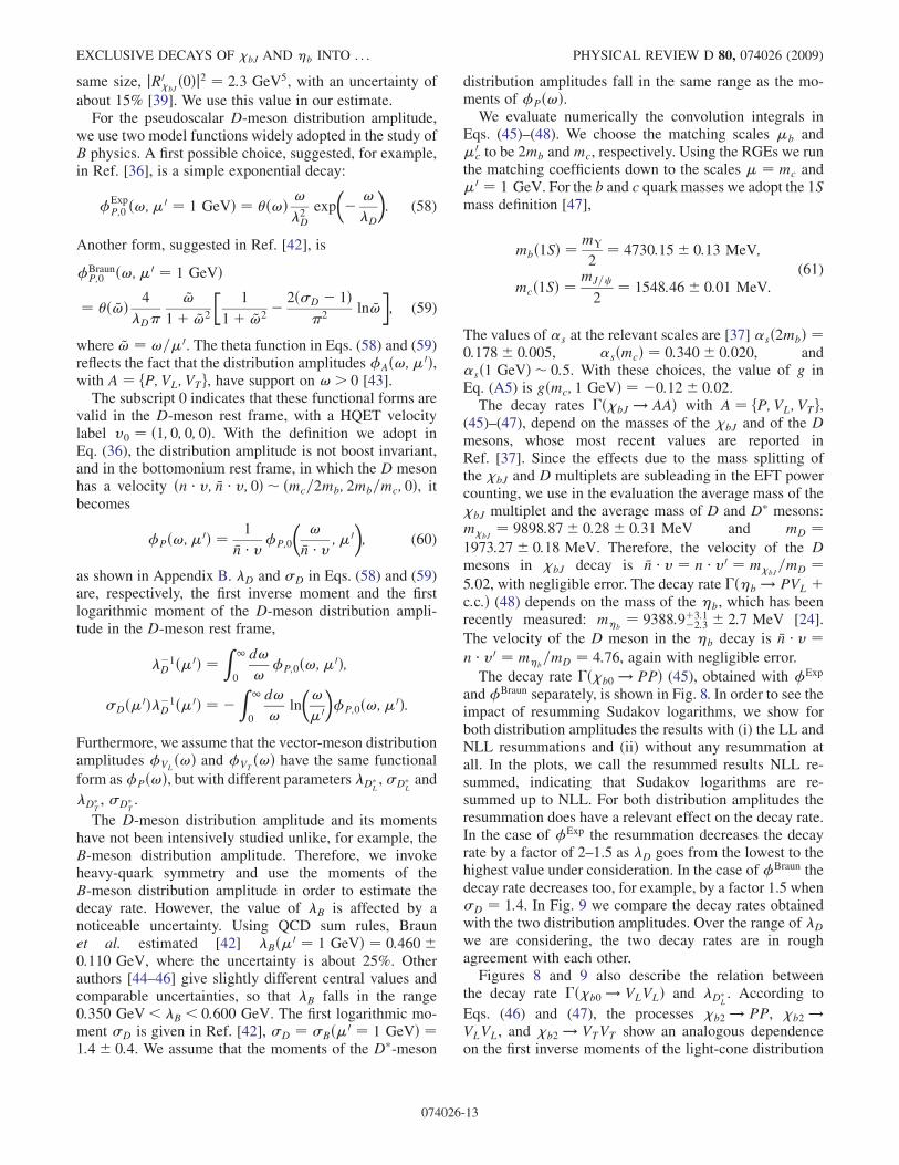
The decay rate �ð�b0 ! PPÞ (45), obtained with Exp

andBraun separately, is shown in Fig. 8. In order to see theimpact of resumming Sudakov logarithms, we show forboth distribution amplitudes the results with (i) the LL andNLL resummations and (ii) without any resummation atall. In the plots, we call the resummed results NLL re-summed, indicating that Sudakov logarithms are re-summed up to NLL. For both distribution amplitudes theresummation does have a relevant effect on the decay rate.In the case of Exp the resummation decreases the decayrate by a factor of 2–1.5 as �D goes from the lowest to thehighest value under consideration. In the case ofBraun thedecay rate decreases too, for example, by a factor 1.5 when�D ¼ 1:4. In Fig. 9 we compare the decay rates obtainedwith the two distribution amplitudes. Over the range of �D

we are considering, the two decay rates are in roughagreement with each other.Figures 8 and 9 also describe the relation between

the decay rate �ð�b0 ! VLVLÞ and �D�L. According to

Eqs. (46) and (47), the processes �b2 ! PP, �b2 !VLVL, and �b2 ! VTVT show an analogous dependenceon the first inverse moments of the light-cone distribution


074026-13

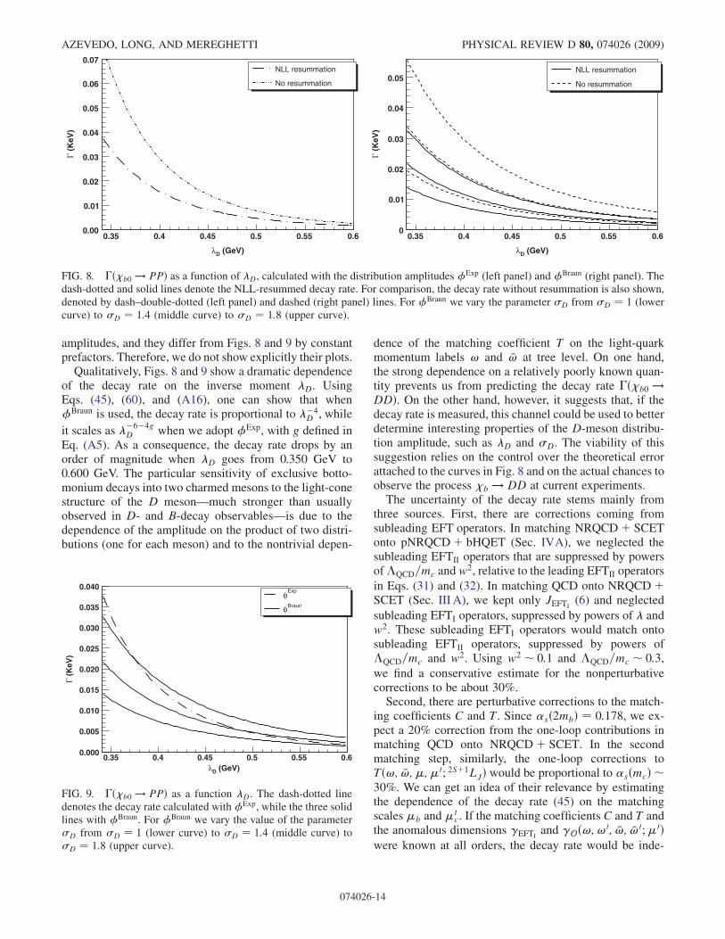
amplitudes, and they differ from Figs. 8 and 9 by constantprefactors. Therefore, we do not show explicitly their plots.

Qualitatively, Figs. 8 and 9 show a dramatic dependenceof the decay rate on the inverse moment �D. UsingEqs. (45), (60), and (A16), one can show that whenBraun is used, the decay rate is proportional to ��4

D , while

it scales as ��6�4gD when we adopt Exp, with g defined in

Eq. (A5). As a consequence, the decay rate drops by anorder of magnitude when �D goes from 0.350 GeV to0.600 GeV. The particular sensitivity of exclusive botto-monium decays into two charmed mesons to the light-conestructure of the D meson—much stronger than usuallyobserved in D- and B-decay observables—is due to thedependence of the amplitude on the product of two distri-butions (one for each meson) and to the nontrivial depen-

dence of the matching coefficient T on the light-quarkmomentum labels ! and �! at tree level. On one hand,the strong dependence on a relatively poorly known quan-tity prevents us from predicting the decay rate �ð�b0 !DDÞ. On the other hand, however, it suggests that, if thedecay rate is measured, this channel could be used to betterdetermine interesting properties of the D-meson distribu-tion amplitude, such as �D and �D. The viability of thissuggestion relies on the control over the theoretical errorattached to the curves in Fig. 8 and on the actual chances toobserve the process �b ! DD at current experiments.The uncertainty of the decay rate stems mainly from

three sources. First, there are corrections coming fromsubleading EFT operators. In matching NRQCDþ SCETonto pNRQCDþ bHQET (Sec. IVA), we neglected thesubleading EFTII operators that are suppressed by powersof�QCD=mc andw

2, relative to the leading EFTII operators

in Eqs. (31) and (32). In matching QCD onto NRQCDþSCET (Sec. III A), we kept only JEFTI

(6) and neglected

subleading EFTI operators, suppressed by powers of � andw2. These subleading EFTI operators would match ontosubleading EFTII operators, suppressed by powers of�QCD=mc and w2. Using w2 � 0:1 and �QCD=mc � 0:3,we find a conservative estimate for the nonperturbativecorrections to be about 30%.Second, there are perturbative corrections to the match-

ing coefficients C and T. Since �sð2mbÞ ¼ 0:178, we ex-pect a 20% correction from the one-loop contributions inmatching QCD onto NRQCDþ SCET. In the secondmatching step, similarly, the one-loop corrections toTð!; �!;�;�0; 2Sþ1LJÞ would be proportional to �sðmcÞ �30%. We can get an idea of their relevance by estimatingthe dependence of the decay rate (45) on the matchingscales�b and�

0c. If the matching coefficients C and T and

the anomalous dimensions �EFTIand �Oð!;!0; �!; �!0;�0Þ

were known at all orders, the decay rate would be inde-

(GeV)Dλ

0.35 0.4 0.45 0.5 0.55 0.6

(K

eV)

Γ

0.00

0.01

0.02

0.03

0.04

0.05

0.06

0.07NLL resummation

No resummation

(GeV)Dλ

0.35 0.4 0.45 0.5 0.55 0.6

(K

eV)

Γ

0

0.01

0.02

0.03

0.04

0.05NLL resummation

No resummation

FIG. 8. �ð�b0 ! PPÞ as a function of �D, calculated with the distribution amplitudes Exp (left panel) and Braun (right panel). Thedash-dotted and solid lines denote the NLL-resummed decay rate. For comparison, the decay rate without resummation is also shown,denoted by dash–double-dotted (left panel) and dashed (right panel) lines. For Braun we vary the parameter �D from �D ¼ 1 (lowercurve) to �D ¼ 1:4 (middle curve) to �D ¼ 1:8 (upper curve).

(GeV)Dλ0.35 0.4 0.45 0.5 0.55 0.6

(K

eV)

Γ

0.000

0.005

0.010

0.015

0.020

0.025

0.030

0.035

0.040ExpφBraunφ

FIG. 9. �ð�b0 ! PPÞ as a function �D. The dash-dotted linedenotes the decay rate calculated withExp, while the three solidlines with Braun. For Braun we vary the value of the parameter�D from �D ¼ 1 (lower curve) to �D ¼ 1:4 (middle curve) to�D ¼ 1:8 (upper curve).


074026-14

pendent of the matching scales �b and �0c. However, since

we only know the first terms in the perturbative expansions,the decay rate bears a residual renormalization-scale de-pendence, whose size is determined by the first neglectedterms.

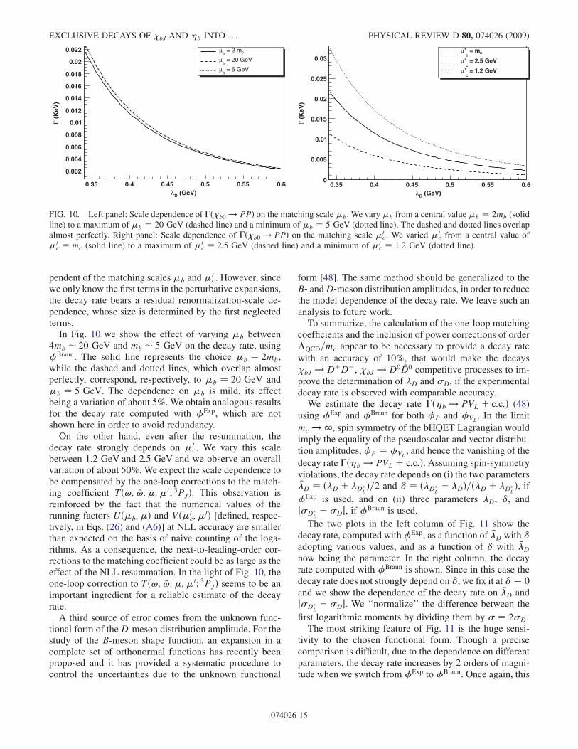
In Fig. 10 we show the effect of varying �b between4mb � 20 GeV and mb � 5 GeV on the decay rate, usingBraun. The solid line represents the choice �b ¼ 2mb,while the dashed and dotted lines, which overlap almostperfectly, correspond, respectively, to �b ¼ 20 GeV and�b ¼ 5 GeV. The dependence on �b is mild, its effectbeing a variation of about 5%. We obtain analogous resultsfor the decay rate computed with Exp, which are notshown here in order to avoid redundancy.

On the other hand, even after the resummation, thedecay rate strongly depends on �0

c. We vary this scalebetween 1.2 GeV and 2.5 GeV and we observe an overallvariation of about 50%. We expect the scale dependence tobe compensated by the one-loop corrections to the match-ing coefficient Tð!; �!;�;�0; 3PJÞ. This observation isreinforced by the fact that the numerical values of therunning factors Uð�b;�Þ and Vð�0

c; �0Þ [defined, respec-

tively, in Eqs. (26) and (A6)] at NLL accuracy are smallerthan expected on the basis of naive counting of the loga-rithms. As a consequence, the next-to-leading-order cor-rections to the matching coefficient could be as large as theeffect of the NLL resummation. In the light of Fig. 10, theone-loop correction to Tð!; �!;�;�0; 3PJÞ seems to be animportant ingredient for a reliable estimate of the decayrate.

A third source of error comes from the unknown func-tional form of the D-meson distribution amplitude. For thestudy of the B-meson shape function, an expansion in acomplete set of orthonormal functions has recently beenproposed and it has provided a systematic procedure tocontrol the uncertainties due to the unknown functional

form [48]. The same method should be generalized to theB- andD-meson distribution amplitudes, in order to reducethe model dependence of the decay rate. We leave such ananalysis to future work.To summarize, the calculation of the one-loop matching

coefficients and the inclusion of power corrections of order�QCD=mc appear to be necessary to provide a decay rate

with an accuracy of 10%, that would make the decays�bJ ! DþD�, �bJ ! D0 �D0 competitive processes to im-prove the determination of �D and �D, if the experimentaldecay rate is observed with comparable accuracy.We estimate the decay rate �ð�b ! PVL þ c:c:Þ (48)

using Exp and Braun for both P and VL. In the limit

mc ! 1, spin symmetry of the bHQET Lagrangian wouldimply the equality of the pseudoscalar and vector distribu-tion amplitudes,P ¼ VL

, and hence the vanishing of the

decay rate �ð�b ! PVL þ c:c:Þ. Assuming spin-symmetryviolations, the decay rate depends on (i) the two parameters��D ¼ ð�D þ �D�

LÞ=2 and � ¼ ð�D�

L� �DÞ=ð�D þ �D�

LÞ, if

Exp is used, and on (ii) three parameters ��D, �, andj�D�

L� �Dj, if Braun is used.

The two plots in the left column of Fig. 11 show thedecay rate, computed withExp, as a function of ��D with �adopting various values, and as a function of � with ��D

now being the parameter. In the right column, the decayrate computed with Braun is shown. Since in this case thedecay rate does not strongly depend on �, we fix it at � ¼ 0and we show the dependence of the decay rate on ��D andj�D�

L� �Dj. We ‘‘normalize’’ the difference between the

first logarithmic moments by dividing them by � ¼ 2�D.The most striking feature of Fig. 11 is the huge sensi-

tivity to the chosen functional form. Though a precisecomparison is difficult, due to the dependence on differentparameters, the decay rate increases by 2 orders of magni-tude when we switch from Exp to Braun. Once again, this

(GeV)Dλ0.35 0.4 0.45 0.5 0.55 0.6

(K

eV)

Γ

0.002

0.004

0.006

0.008

0.01

0.012

0.014

0.016

0.018

0.02

0.022 b = 2 mb

µ = 20 GeV

bµ

= 5 GeVb

µ

(GeV)Dλ0.35 0.4 0.45 0.5 0.55 0.6

(K

eV)

Γ

0

0.005

0.01

0.015

0.02

0.025

0.03c = m

c’µ

= 2.5 GeVc’µ

= 1.2 GeVc’µ

FIG. 10. Left panel: Scale dependence of �ð�b0 ! PPÞ on the matching scale �b. We vary�b from a central value�b ¼ 2mb (solidline) to a maximum of �b ¼ 20 GeV (dashed line) and a minimum of �b ¼ 5 GeV (dotted line). The dashed and dotted lines overlapalmost perfectly. Right panel: Scale dependence of �ð�b0 ! PPÞ on the matching scale �0

c. We varied �0c from a central value of

�0c ¼ mc (solid line) to a maximum of �0

c ¼ 2:5 GeV (dashed line) and a minimum of �0c ¼ 1:2 GeV (dotted line).


074026-15

effect hinders our ability to predict �ð�b ! PVL þ c:c:Þbut it opens up the interesting possibility to discriminatebetween different model distribution amplitudes.

Using Eqs. (48) and (A17), we know that �ð�b !PVL þ c:c:Þ goes like ��4�4g

D when Exp is used or ��4D

when Braun is used. Figure 11 appears to confirm thisstrong dependence on ��D. The plots in the lower half ofFig. 11 reflect the fact that the decay rate vanishes if oneassumes Pð!Þ ¼ VL

ð!Þ.We conclude this section with the determination of the

branching ratiosBð�b0 ! PPÞ ¼ �ð�b0 ! PPÞ=�ð�b0 !light hadronsÞ and Bð�b ! PVL þ c:c:Þ ¼ �ð�b !PVL þ c:c:Þ=�ð�b ! light hadronsÞ. At leading order inpNRQCD, the only nonperturbative parameter involvedin the inclusive decay width of the �b is jR�b

ð0Þj2 [4],

�ð�b ! light hadronsÞ ¼ 2 Imf1ð1S0Þm2

b

Nc

2jR�b

ð0Þj2:(62)

Therefore, Bð�b ! PVL þ c:c:Þ does not depend on the

quarkonium wave function, and the only nonperturbativeparameters in Bð�b ! PVL þ c:c:Þ are those describingthe D-meson distribution amplitudes.For P-wave states, the inclusive decay rate was obtained

in Refs. [4,49], where the contributions of the configura-tions in which the quark-antiquark pair is in a color-octetS-wave state were first recognized. In pNRQCD the inclu-sive decay rate is written as [50,51]

�ð�b0 ! light hadronsÞ¼ 1

m4b

3Nc

jR0

�bð0Þj2

�Imf1ð3P0Þ þ

1

9N2c

Imf8ð3S1ÞE�;

(63)

where the color-octet matrix element has been expressed interms of the heavy quarkonium wave function and of thegluonic correlator E, whose precise definition is given inRef. [50]. E is a universal parameter and is completelyindependent of any particular heavy quarkonium stateunder consideration. Its value has been obtained by fitting

(GeV)Dλ

0.35 0.4 0.45 0.5 0.55 0.6

(K

eV)

Γ

0

0.1

0.2

0.3

0.4

0.5

0.6-310×

= -0.15δ = -0.1δ = 0.1δ = 0.15δ

(GeV)Dλ

0.35 0.4 0.45 0.5 0.55 0.6

(K

eV)

Γ

0

0.02

0.04

0.06

0.08

0.1

0.12

0.14

0.16 = 0.05 σ|/Dσ - LD*σ|

= 0.1σ|/Dσ - LD*σ|

= 0.15σ|/Dσ - LD*σ|

δ

-0.15 -0.1 -0.05 0 0.05 0.1 0.15

(K

eV)

Γ

0

0.2

0.4

0.6

0.8

1

-310×

= 0.300 GeVDλ = 0.400 GeVDλ = 0.500 GeVDλ = 0.600 GeVDλ

σ|/Dσ - LD*σ|

0 0.02 0.04 0.06 0.08 0.1 0.12 0.14

(K

eV)

Γ

0

0.05

0.1

0.15

0.2

0.25

= 0.300 GeVDλ

= 0.400 GeVDλ = 0.500 GeVDλ = 0.600 GeVDλ

FIG. 11 (color online). Left panel: �ð�b ! PVL þ c:c:Þ as a function of �D and �, computed using exponential distribution

amplitudes ExpP and

ExpVL

. Right panel: �ð�b ! PVL þ c:c:Þ as a function of �D and j�D�L� �Dj=�, computed with the Braun

distribution amplitudes BraunP and Braun

VL.


074026-16

to existing charmonium data and, thanks to the universal-ity, the same value can be used to predict properties ofbottomonium decays. It is found in Ref. [50] that E ¼5:3þ3:5

�2:2. The matching coefficients in Eqs. (62) and (63)

are known to one loop. For the updated value we refer toRef. [52] and references therein. For reference, the tree-level values of the coefficients are as follows [4]:

Imf1ð1S0Þ ¼ �2sð2mbÞ CF

2Nc

;

Imf1ð3P0Þ ¼ 3�2sð2mbÞ CF

2Nc

;

Imf8ð3S1Þ ¼nf6�2sð2mbÞ:

(64)

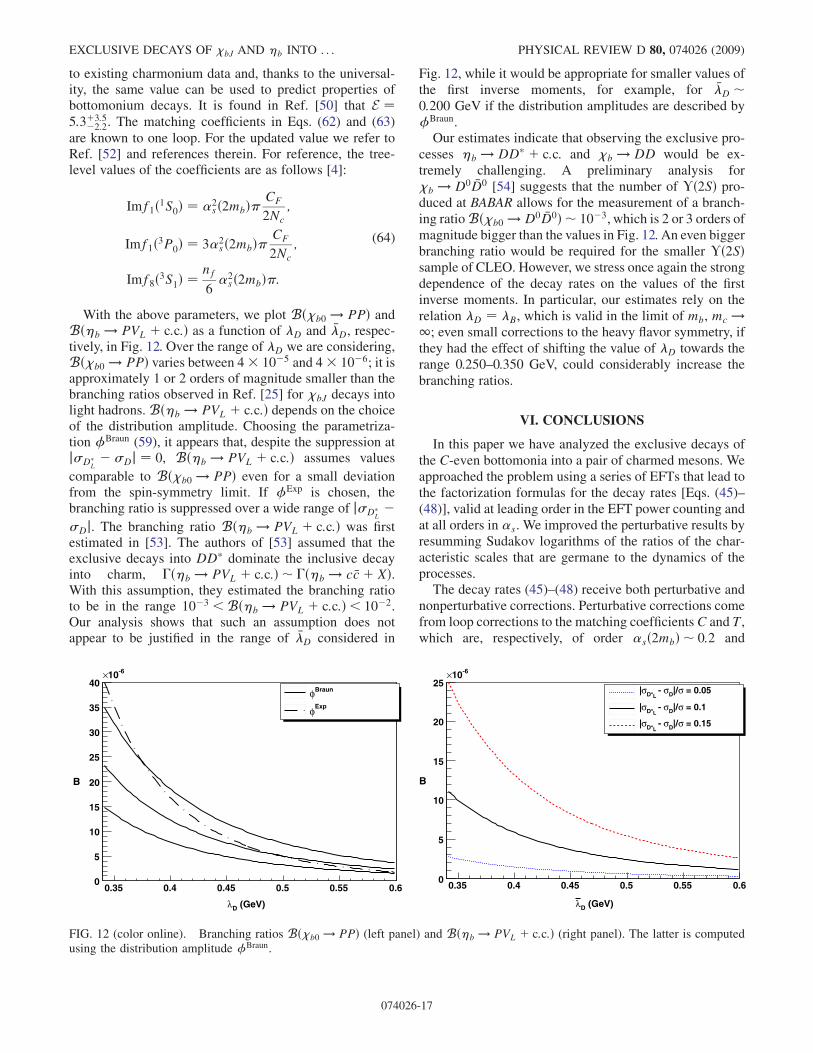
With the above parameters, we plot Bð�b0 ! PPÞ andBð�b ! PVL þ c:c:Þ as a function of �D and ��D, respec-tively, in Fig. 12. Over the range of �D we are considering,Bð�b0 ! PPÞ varies between 4 10�5 and 4 10�6; it isapproximately 1 or 2 orders of magnitude smaller than thebranching ratios observed in Ref. [25] for �bJ decays intolight hadrons.Bð�b ! PVL þ c:c:Þ depends on the choiceof the distribution amplitude. Choosing the parametriza-tion Braun (59), it appears that, despite the suppression atj�D�

L� �Dj ¼ 0, Bð�b ! PVL þ c:c:Þ assumes values

comparable to Bð�b0 ! PPÞ even for a small deviationfrom the spin-symmetry limit. If Exp is chosen, thebranching ratio is suppressed over a wide range of j�D�

L�

�Dj. The branching ratio Bð�b ! PVL þ c:c:Þ was firstestimated in [53]. The authors of [53] assumed that theexclusive decays into DD� dominate the inclusive decayinto charm, �ð�b ! PVL þ c:c:Þ � �ð�b ! c �cþ XÞ.With this assumption, they estimated the branching ratioto be in the range 10�3 <Bð�b ! PVL þ c:c:Þ< 10�2.Our analysis shows that such an assumption does notappear to be justified in the range of ��D considered in

Fig. 12, while it would be appropriate for smaller values ofthe first inverse moments, for example, for ��D �0:200 GeV if the distribution amplitudes are described byBraun.Our estimates indicate that observing the exclusive pro-

cesses �b ! DD� þ c:c: and �b ! DD would be ex-tremely challenging. A preliminary analysis for�b ! D0 �D0 [54] suggests that the number of �ð2SÞ pro-duced at BABAR allows for the measurement of a branch-ing ratioBð�b0 ! D0 �D0Þ � 10�3, which is 2 or 3 orders ofmagnitude bigger than the values in Fig. 12. An even biggerbranching ratio would be required for the smaller �ð2SÞsample of CLEO. However, we stress once again the strongdependence of the decay rates on the values of the firstinverse moments. In particular, our estimates rely on therelation �D ¼ �B, which is valid in the limit of mb, mc !1; even small corrections to the heavy flavor symmetry, ifthey had the effect of shifting the value of �D towards therange 0.250–0.350 GeV, could considerably increase thebranching ratios.

VI. CONCLUSIONS

In this paper we have analyzed the exclusive decays ofthe C-even bottomonia into a pair of charmed mesons. Weapproached the problem using a series of EFTs that lead tothe factorization formulas for the decay rates [Eqs. (45)–(48)], valid at leading order in the EFT power counting andat all orders in �s. We improved the perturbative results byresumming Sudakov logarithms of the ratios of the char-acteristic scales that are germane to the dynamics of theprocesses.The decay rates (45)–(48) receive both perturbative and

nonperturbative corrections. Perturbative corrections comefrom loop corrections to the matching coefficients C and T,which are, respectively, of order �sð2mbÞ � 0:2 and

(GeV)Dλ

0.35 0.4 0.45 0.5 0.55 0.60

5

10

15

20

25

30

35

40-610×

BraunφExpφ

B

(GeV)Dλ

0.35 0.4 0.45 0.5 0.55 0.60

5

10

15

20

25-610×

= 0.05σ|/Dσ - LD*σ|

= 0.1σ|/Dσ - LD*σ|

= 0.15σ|/Dσ - LD*σ|

B

FIG. 12 (color online). Branching ratios Bð�b0 ! PPÞ (left panel) and Bð�b ! PVL þ c:c:Þ (right panel). The latter is computedusing the distribution amplitude Braun.


074026-17

�sðmcÞ � 0:3. The largest nonperturbative contributioncould be as big as �QCD=mc, which would amount ap-

proximately to a 30% correction. Therefore, corrections tothe leading-order decay rates could be noticeable, as thestrong dependence of the decay rates on the renormaliza-tion scale �0

c suggests. However, the EFT approach shownin this paper allows for a systematic treatment of bothperturbative corrections and power-suppressed operators,so that, if the experimental data require, it is possible toextend the present analysis beyond the leading order.

For simplicity, we have focused in this paper on thedecays of C-even bottomonia, in which cases the decaysproceed via two intermediate gluons, and both the match-ing coefficients C and T are nontrivial at tree level. Thesame EFT approach can be applied to the decays of C-oddstates, in particular, to the decays � ! DD and � !D�D�, with the complication that the matching coefficientT arises only at one-loop level. Moreover, the same EFTformalism developed in this paper can be applied to thestudy of the channels that have vanishing decay rates atleading order in the power counting, such as �b ! D�D�,� ! DD� þ c:c:, and �b2 ! DD� þ c:c:. Experimentaldata for the charmonium system show that, for the decaysof charmonium into light hadrons, the expected suppres-sion of the subleading twist processes is not seen. It isinteresting to see whether such an effect appears in botto-monium decays into two charmed mesons, using the EFTapproach of this paper to evaluate the power-suppresseddecay rates.

Finally, in Sec. V we used model distribution amplitudesto estimate the decay rates. The most evident, qualitativefeature of the decay rates is the strong dependence on theparameters of the D-meson distribution amplitude. Eventhough this feature may prevent us from giving reliableestimates of the decay rates or of the branching ratios, itmakes the channels analyzed here ideal candidates for theextraction of important D-meson parameters, when thebranching ratios can be observed with sufficient accuracy.

ACKNOWLEDGMENTS

We would like to thank S. Fleming for proposing thisproblem and for countless useful discussions, N. Brambillaand A. Vairo for suggestions and comments, and R. Briere,V.M. Braun, and S. Stracka for helpful communications.Bw. L. is grateful for the hospitality of the University ofArizona, where part of this work was finished. This re-search was supported by the US Department of Energyunder Grant No. DE-FG02-06ER41449 (R.A. and E.M.)and No. DE-FG02-04ER41338 (R.A., Bw. L. and E.M.).

APPENDIX A: SOLUTION OF THE RUNNINGEQUATION IN pNRQCDþ bHQET

The RGE in Eq. (57) can be solved by applying themethods discussed in Ref. [36] to find the evolution of the

B-meson distribution amplitude. We generalize this ap-proach to the specific case discussed here, where twodistribution amplitudes are present. Following Ref. [36],we define

!�ð!;!0; �sÞ ¼ ��sCF

��ð!�!0Þ

�1

!�!0

�þ

þ �ð!0 �!Þ�ð!Þ !!0

�1

!0 �!

�þ

�:

Lange and Neubert [36] prove that

Zd!0!�ð!;!0; �sÞð!0Þa ¼ !aF ða;�sÞ; (A1)

with

F ða;�sÞ ¼ �sCF

½c ð1þ aÞ þ c ð1� aÞ þ 2�E:

c is the digamma function and �E the Euler constant.Equation (A1) is valid if �1< Re a < 1. Exploiting(A1), a solution of the running equation (57) with the initialcondition Tð!; �!;�0

0Þ ¼ ð!=�00Þ�ð �!=�0

0Þ� at a certain

scale �00 is

F2ð�0ÞTð!; �!;�0Þ ¼ F2ð�00Þfð!;�0;�0

0;�Þfð �!;�0;�00; �Þ;(A2)

with

fð!;�0; �00; �Þ ¼

�!

�00

��gð �n � vÞg expUð�0

0; �0; �Þ;

g � gð�00; �

0Þ ¼Z �sð�0Þ

�sð�00Þ

d�

�ð�Þ�cuspð�Þ;

Uð�00; �

0; �Þ ¼Z �sð�0Þ

�sð�00Þ

d�

�ð�Þ��cuspð�Þ

Z �

�sð�00Þ

d�0

�ð�0Þþ �1ð�Þ þF ð�� g;�Þ

�;

�1ð�sÞ ¼ �2�sCF

4: (A3)

The function fð �!;�0; �00; �Þ has the same form as

fð!;�0; �00; �Þ and is obtained by replacing ! ! �!, � !

�, and �n � v ! n � v0 in Eq. (A3). The integrals over � canbe performed explicitly using the beta function in Eq. (28).The result is

fð!;�0; �00; �Þfð �!;�0; �0

0; �Þ

¼�!

�00

��g

��!

�00

��gð �n � vn � v0Þg exp½Vð�0

0; �0Þ

�ð1� �þ gÞ�ð1þ �Þ�ð1þ �� gÞ�ð1� �Þ

�ð1� �þ gÞ�ð1þ �Þ�ð1þ �� gÞ�ð1� �Þ ;

(A4)

where, at NLL,


074026-18

gð�00; �

0Þ ¼ ��ð0Þcusp

2�0

�lnrþ

��ð1Þcusp

�ð0Þcusp

� �1

�0

��sð�0

0Þ4

ðr� 1Þ�

(A5)

and

Vð�00; �

0Þ ¼ ��ð0Þcusp

2

�20

�r� 1� r lnr

�sð�0Þ þ��ð1Þcusp

�ð0Þcusp

� �1

�0

�

1� rþ lnr

4þ �1

8�0

ln2r

�

þ CF

�0

ð2� 8�EÞ lnr; (A6)

with r ¼ �sð�0Þ=�sð�00Þ. Notice that in the running from

�00 ¼ mc to�

0 ¼ 1 GeV only three flavors are active, so in

the expressions for �0, �1, and �ð1Þcusp, we use nf ¼ 3.

Equation (A4) is the solution for the initial conditionTð!; �!;�0

0Þ ¼ ð!=�00Þ�ð �!=�0

0Þ�. To solve the RGE for a

generic initial condition, we express T as the Fourier trans-form with respect to ln!=�0

0,

Tð!; �!;�00Þ ¼

1

ð2Þ2Z þ1

�1drds exp

��ir ln

!

�00

�

exp

��is ln

�!

�00

�F½Tðr; s; �0

0Þ

¼ 1

ð2Þ2Z þ1

�1drds

�!

�00

��ir��!

�00

��isF½T

ðr; s; �00Þ;

where F½T denotes the Fourier transform of T. From thesolutions (A2)–(A4) it follows that

F2ð�0ÞTð!; �!;�0Þ ¼ F2ð�00Þ

ð2Þ2Z þ1

�1drds

�!

�00

��ir�g

��!

�00

��is�gð �n � vn � v0ÞgF½T

ðr; s; �00Þ exp½Vð�0

0; �0Þ

�ð1þ irþ gÞ�ð1� irÞ�ð1� ir� gÞ�ð1þ irÞ

�ð1þ isþ gÞ�ð1� isÞ�ð1� is� gÞ�ð1þ isÞ : (A7)

The Fourier transform of the matching coefficient inEq. (A7) has to be understood in the sense of distributions[55]. That is, we define the Fourier transform of T as thefunction of r and s that satisfies

1

ð2Þ2Z

drdsF½Tðr; s; �0Þ’Aðr;�0Þ’Bðs;�0Þ

¼Z þ1

0

d!

!

d �!

�!Tð!; �!;�0ÞAð!;�0ÞBð �!;�0Þ;

(A8)

or, more precisely, F½Tðr; s; �0Þ is the linear functionalthat acts on the test functions ’AðrÞ and ’BðsÞ according to

1

ð2Þ2 ðF½Tðr; s; �0Þ; ’Aðr;�0Þ’Bðs;�0ÞÞ

¼Z þ1

0

d!

!

d �!

�!Tð!; �!;�0ÞAð!;�0ÞBð �!;�0Þ:

(A9)

The function ’A is the Fourier transform of the D-mesondistribution amplitude,

’Aðr;�0Þ ¼Z 1

0

d!

!

�!

�0

�irAð!;�0Þ; (A10)

where the integral on the r.h.s. should converge in theordinary sense because of the regularity properties of theD-meson distribution amplitude. As in Sec. IV, the sub-script A denotes the spin and polarization of the D meson.In the distribution sense, the Fourier transform of the

coefficient 1=ð!þ �!Þ is

F

�1

!þ �!

�ðr; s; �0

0Þ ¼ ð2Þ2 1

2�00

�ðrþ sþ iÞ

sech

�

2ðr� sÞ

�

¼ 1

2ð2Þ2 1

2�00

�ðRþ iÞ sech�

2S

�;

(A11)

where R ¼ rþ s, S ¼ r� s, and the factor 12 comes from

the Jacobian of the change of variables. The hyperbolicsecant is defined as sech ¼ 1= cosh. Similarly, we find

F

�!� �!

!þ �!

�ðR; S;�0

0Þ ¼i

2ð2Þ2�ðRÞ

�cosech

�

2Sþ i"

�

þ cosech

�

2S� i"

��: (A12)

The � function in Eq. (A11) has a complex argument.The definition is analogous to the one in real space [55],

ð�ðRþ iÞ; ’ðRÞÞ ¼ ’ð�iÞ: (A13)

Using Eqs. (A11) and (A12), we can perform the integral inEq. (A7), obtaining, respectively, Tð!; �!;�;�0; 3PJÞ andTð!; �!;�;�0; 1S0Þ. In order to give an explicit example,

we proceed using Eq. (A11). Integrating the � function weare left with


074026-19

F2ð�0ÞTð!; �!;�0Þ ¼ F2ð�00Þ exp½Vð�0

0; �0Þ 1

�00

��02

0

! �!

�1=2þgð �n � vn � v0Þg

Z 1

�1dS exp

��i

S

2ln!

�!

�

sech

�

2S

�1

1þ S2�ð32 þ gþ i

2SÞ�ð12 � g� i

2SÞ�ð32 þ g� i

2SÞ�ð12 � gþ i

2SÞ: (A14)

The integral (A14) can be done by contour. The integrand has poles along the imaginary axis. In S ¼ �i there is adouble pole, coming from the coincidence of one pole of the hyperbolic secant and the singularities in 1=ð1þ S2Þ. The �functions in the numerator have poles, respectively, in S ¼ �ið2nþ 3þ 2gÞ with n > 0, while the other poles of sech arein S ¼ �ið2nþ 1Þ with n � 1. We close the contour in the upper half plane for �!>! and in the lower half plan for!> �!, obtaining

F2ð�0ÞTð!; �!;�0Þ ¼ F2ð�00Þ exp½Vð�0

0; �0Þ�ð �!�!Þ 1

�!

��02

0 �n � vn � v0

! �!

�g

��ð1þ gÞ�ð2þ gÞ�ð1� gÞ�ð�gÞ

�1� ln

!

�!þ c ð1� gÞ � c ð�gÞ þ c ð1þ gÞ � c ð2þ gÞ

�

þ X1n¼1

ð�Þnþ1

�!

�!

�n 1

nðnþ 1Þ�ð1� nþ gÞ�ð2þ nþ gÞ�ð�n� gÞ�ð1� gþ nÞ

� X1n¼1

�!

�!

�nþg

ðn� 1Þ! cscðgÞ 1

ðnþ gÞð1þ nþ gÞ�ð2þ nþ 2gÞ

�ð1þ nÞ�ð�n� 2gÞ�þ ð! ! �!Þ; (A15)

with cscðgÞ ¼ 1= sinðgÞ, and c is the digamma function. More compactly, we can express Eq. (A15) using thehypergeometric functions 4F3 and 3F2,

F2ð�0ÞTð!; �!;�;�0; 3PJÞ ¼ F2ð�0cÞCF

N2c

4�sð�0cÞ

mb

exp½Vð�0c; �

0Þ��02

c �n � vn � v0

! �!

�g �ð �!�!Þ

�!

��ð1þ gÞ�ð2þ gÞ�ð1� gÞ�ð�gÞ

�1� ln

!

�!þ c ð1� gÞ � c ð�gÞ þ c ð1þ gÞ � c ð2þ gÞ

�

þ 1

2

!

�!

�ðgþ 2Þ�ðgþ 3Þ�ð1� gÞ�ð2� gÞ 4F3

�1; 1; gþ 2; gþ 3; 3; 1� g; 2� g;�!

�!

�

��!

�!

�1þg

4 cosðgÞ�ð2þ 2gÞ2gþ 2 3F2

�gþ 1; 2gþ 2; 2gþ 3; 2; gþ 3;�!

�!

��þ ð! ! �!Þ;

(A16)

where we have introduced the constants that appear in the initial condition in Eq. (33). In the same way, we obtain

F2ð�0ÞTð!; �!;�;�0; 1S0Þ ¼ F2ð�0cÞ CF

2N2c

4�sð�0cÞ

mb

exp½Vð�0c; �

0Þ�ð �!�!Þ��02

c �n � vn � v0

! �!

�g

�2�ð1þ gÞ�ð2þ gÞ�ð1� gÞ�ð2� gÞ

!

�! 3F2

�1; gþ 1; gþ 2; 1� g; 2� g;�!

�!

�þ �2ð1þ gÞ

�2ð1� gÞ�

�!

�!

�1þg

4 cosðgÞ�ð1þ 2gÞ�ð2gþ 2Þ2F1

�2gþ 2; 2gþ 1; 2;�!

�!

�� ð! ! �!Þ: (A17)

In Eqs. (A16) and (A17) we renamed the initial scale�0

0 ¼ �0c to denote its connection to the scale mc. Setting

�0 ¼ �0c or, equivalently, g ¼ 0, it can be explicitly veri-

fied that the solutions (A16) and (A17) satisfy the initialconditions (33).

APPENDIX B: BOOST TRANSFORMATION OFTHE D-MESON DISTRIBUTION AMPLITUDE

We derive in this appendix the relation between thedistribution amplitudes in the D-meson and in the botto-monium rest frames, as given in Eq. (60). In the D-meson


074026-20

rest frame, characterized by the velocity label v0 ¼ð1; 0; 0; 0Þ, the local heavy-light matrix element is definedas

h0j ��lnð0Þ

�6n2�5h

cnð0ÞjDiv0

¼ �iFð�0Þ �n � v0

2: (B1)

The matrix element of the heavy- and light-quark fields at alightlike separation z

�0 ¼ n � z0 �n�=2 defines the light-cone

distribution ~0ðn � z0; �0Þ in coordinate space:

h0j ��lnðn � z0Þ

�6n2�5H c

nð0ÞjDiv0

¼ �iFð�0Þ �n � v0

2~0ðn � z0; �0Þ: (B2)

Equations (B1) and (B2) imply ~0ð0; �0Þ ¼ 1. In the defi-nitions (B1) and (B2) the subscript 0 is used to denotequantities in the D-meson rest frame. This convention isused in the rest of this appendix. In the bottomonium restframe, where the velocity label in light-cone coordinates isv ¼ ðn � v; �n � v; 0Þ and the lightlike separation is z� ¼ n �z �n�=2, we define

h0j ��lnð0Þ

�6n2�5h

cnð0ÞjDiv ¼ �iFð�0Þ �n � v

2(B3)

and

h0j ��lnðn � zÞ

�6n2�5H c

nð0ÞjDiv ¼ �iFð�0Þ �n � v2

~ðn � z; �0Þ:(B4)

Suppose that� is some standardized boost that takes theD meson from v, its velocity in the bottomonium restframe, to rest. It is straightforward to find the relationsbetween the D-meson momenta in the two frames:

n � p0 ¼ �n � vn � p and �n � p0 ¼ n � v �n � p:There is a similar relation for the light-cone coordinates,

n � z0 ¼ �n � vn � z:With Uð�Þ, the unitary operator that implements the boost�, one can write

Uð�ÞjDiv ¼ jDiv0:

We choose � such that, for the Dirac fields,

Uð�Þ��lnðxÞU�1ð�Þ ¼ ��1

1=2��lð�xÞ and

Uð�ÞhcnðxÞU�1ð�Þ ¼ ��11=2h

cð�xÞ;where

�1=2 ¼ cosh�

2þ

�6n6n� 6n �6n4

sinh�

2;

with � related to v by e� ¼ �n � v and e�� ¼ n � v.Now we can write the matrix element in Eq. (B3) as

h0j ��ln

�6n2�5h

cnð0ÞjDiv ¼ h0jU�1ð�ÞðUð�Þ ��l

nð0ÞU�1ð�ÞÞ�6n2�5ðUð�Þhcnð0ÞU�1ð�ÞÞUð�ÞjDiv

¼ h0j ��lð0Þ�1=2

�6n2�5�

�11=2h

cð0ÞjDiv0¼ �n � vh0j ��lð0Þ

�6n2�5h

cð0ÞjDiv0¼ �iFð�0Þ �n � v

2�n � v0

¼ �iFð�0Þ �n � v2

; (B5)

where, in the last step, we have used �n � v0 ¼ 1. Equation (B5) is thus in agreement with the definition in Eq. (B3).Applying the same reasoning to Eq. (B4), one finds

h0j ��lnðn � zÞ

�6n2�5H c

nð0ÞjDiv ¼ �n � vh0j ��lð �n � vn � zÞ�6n2�5H cð0ÞjDiv0

¼ �iFð�0Þ �n � v2

~0ðn � z0; �0Þ: (B6)

Comparing Eq. (B6) with (B4), we see that ~ðn � z; �0Þ ¼ ~0ð �n � vn � z;�0Þ. Note that in the bottomonium rest frame thenormalization condition for the distribution amplitude is also ~ð0; �0Þ ¼ 1.

In the main text of this paper we have used the D-meson distribution amplitudes in momentum space,

0ð!0; �0Þ � 1

2

Zdn � z0ei!0n�z0 ~0ðn � z0; �0Þ; ð!;�0Þ � 1

2

Zdn � zei!n�z ~ðn � z;�0Þ:

Using Eq. (B6), we can relate the two distributions:


074026-21

ð!;�0Þ ¼ 1

2

Zdn � zei!n�z ~ðn � z;�0Þ ¼ 1

2

Zdn � zei!n�z ~0ð �n � vn � z; �0Þ

¼ 1

2

1

�n � vZ

dn � zeið!=ð �n�vÞÞn�z ~0ðn � z;�0Þ ¼ 1

�n � v0

�!

�n � v ;�0�;

as stated in Eq. (60). The D-meson light-cone distribution is normalized to 1 in both frames,Zd!00ð!0; �

0Þ ¼Z

d!ð!;�0Þ ¼ 1;

as can be easily proved using ~0ð0; �0Þ ¼ ~ð0; �0Þ ¼ 1.

[1] V. L. Chernyak and A. R. Zhitnitsky, Phys. Rep. 112, 173(1984).

[2] S. J. Brodsky and G. P. Lepage, Adv. Ser. Dir. High EnergyPhys. 5, 93 (1989).

[3] N. Brambilla et al. (Quarkonium Working Group), arXiv:hep-ph/0412158.

[4] G. T. Bodwin, E. Braaten, and G. P. Lepage, Phys. Rev. D51, 1125 (1995); 55, 5853(E) (1997).

[5] C.W. Bauer, S. Fleming, and M. E. Luke, Phys. Rev. D 63,014006 (2000).

[6] C.W. Bauer, S. Fleming, D. Pirjol, and I.W. Stewart,Phys. Rev. D 63, 114020 (2001).

[7] C.W. Bauer, D. Pirjol, and I.W. Stewart, Phys. Rev. D 65,054022 (2002).

[8] C.W. Bauer, S. Fleming, D. Pirjol, I. Z. Rothstein, andI.W. Stewart, Phys. Rev. D 66, 014017 (2002).

[9] A. K. Leibovich, Z. Ligeti, and M. B. Wise, Phys. Lett. B564, 231 (2003).

[10] A. Pineda and J. Soto, Nucl. Phys. B, Proc. Suppl. 64, 428(1998).

[11] N. Brambilla, A. Pineda, J. Soto, and A. Vairo, Nucl. Phys.B566, 275 (2000).

[12] N. Brambilla, A. Pineda, J. Soto, and A. Vairo, Rev. Mod.Phys. 77, 1423 (2005).

[13] B. Grinstein, Nucl. Phys. B339, 253 (1990).[14] E. Eichten and B. R. Hill, Phys. Lett. B 234, 511

(1990).[15] H. Georgi, Phys. Lett. B 240, 447 (1990).[16] M. Beneke, A. P. Chapovsky, A. Signer, and G.

Zanderighi, Phys. Rev. Lett. 93, 011602 (2004).[17] M. Beneke, A. P. Chapovsky, A. Signer, and G.

Zanderighi, Nucl. Phys. B686, 205 (2004).[18] S. Fleming, A. H. Hoang, S. Mantry, and I.W. Stewart,

Phys. Rev. D 77, 074010 (2008).[19] S. Fleming, A. H. Hoang, S. Mantry, and I.W. Stewart,

Phys. Rev. D 77, 114003 (2008).[20] G. T. Bodwin, E. Braaten, D. Kang, and J. Lee, Phys. Rev.

D 76, 054001 (2007).[21] D. Kang, T. Kim, J. Lee, and C. Yu, Phys. Rev. D 76,

114018 (2007).[22] V. V. Braguta, A.K. Likhoded, and A.V. Luchinsky,

arXiv:0902.0459.[23] V. V. Braguta and V.G. Kartvelishvili, arXiv:0907.2772.

[24] B. Aubert et al. (BABAR Collaboration), Phys. Rev. Lett.101, 071801 (2008); 102, 029901(E) (2009).

[25] D.M. Asner et al., Phys. Rev. D 78, 091103 (2008).[26] R. A. Briere et al. (CLEO Collaboration), Phys. Rev. D 78,

092007 (2008).[27] R. J. Hill, Phys. Rev. D 73, 014012 (2006).[28] M. E. Luke and A.V. Manohar, Phys. Rev. D 55, 4129

(1997).[29] M. E. Luke, A.V. Manohar, and I. Z. Rothstein, Phys. Rev.

D 61, 074025 (2000).[30] A. V. Manohar and I.W. Stewart, Phys. Rev. D 62, 014033

(2000).[31] A. H. Hoang and I.W. Stewart, Phys. Rev. D 67, 114020

(2003).[32] A. Manohar and M. Wise, Heavy Quark Physics

(Cambridge University Press, Cambridge, 2000).[33] A. V. Manohar and I.W. Stewart, Phys. Rev. D 76, 074002

(2007).[34] G. P. Korchemsky and A.V. Radyushkin, Nucl. Phys.

B283, 342 (1987); I. A. Korchemskaya and G. P.Korchemsky, Phys. Lett. B 287, 169 (1992).

[35] B. I. Eisenstein et al. (CLEO Collaboration), Phys. Rev. D78, 052003 (2008).

[36] B. O. Lange and M. Neubert, Phys. Rev. Lett. 91, 102001(2003).

[37] C. Amsler et al. (Particle Data Group), Phys. Lett. B 667, 1(2008).

[38] R. Barbieri, R. Gatto, R. Kogerler, and Z. Kunszt, Phys.Lett. 57B, 455 (1975); W. Celmaster, Phys. Rev. D 19,1517 (1979).

[39] G. T. Bodwin, D. K. Sinclair, and S. Kim, Phys. Rev. D 65,054504 (2002).

[40] E. J. Eichten and C. Quigg, Phys. Rev. D 52, 1726 (1995).[41] W. Buchmuller and S.H. H. Tye, Phys. Rev. D 24, 132

(1981).[42] V.M. Braun, D. Y. Ivanov, and G. P. Korchemsky, Phys.

Rev. D 69, 034014 (2004).[43] A. G. Grozin and M. Neubert, Phys. Rev. D 55, 272

(1997).[44] M. Beneke, G. Buchalla, M. Neubert, and C. T. Sachrajda,

Phys. Rev. Lett. 83, 1914 (1999).[45] S. J. Lee and M. Neubert, Phys. Rev. D 72, 094028 (2005).[46] V. Pilipp, arXiv:hep-ph/0703180.


074026-22

[47] A. H. Hoang, Z. Ligeti, and A.V. Manohar, Phys. Rev.Lett. 82, 277 (1999).

[48] Z. Ligeti, I.W. Stewart, and F. J. Tackmann, Phys. Rev. D78, 114014 (2008).

[49] G. T. Bodwin, E. Braaten, and G. P. Lepage, Phys. Rev. D46, R1914 (1992).

[50] N. Brambilla, D. Eiras, A. Pineda, J. Soto, and A. Vairo,Phys. Rev. Lett. 88, 012003 (2001).

[51] N. Brambilla, D. Eiras, A. Pineda, J. Soto, and A. Vairo,Phys. Rev. D 67, 034018 (2003).

[52] A. Vairo, Mod. Phys. Lett. A 19, 253 (2004).[53] F. Maltoni and A.D. Polosa, Phys. Rev. D 70, 054014

(2004).[54] S. Stracka (private communication).[55] I.M. Gelfand and G. E. Shilov, Generalized Functions

(Academic Press, New York, 1964), Vol. 1.


074026-23