Download pdf - Knowledge-based Vision in Man and Machine || Generative Models for Discovering Sparse Distributed Representations

Generative Models for Discovering Sparse Distributed RepresentationsAuthor(s): Geoffrey E. Hinton and Zoubin GhahramaniSource: Philosophical Transactions: Biological Sciences, Vol. 352, No. 1358, Knowledge-basedVision in Man and Machine (Aug. 29, 1997), pp. 1177-1190Published by: The Royal SocietyStable URL: http://www.jstor.org/stable/56656 .

Accessed: 07/05/2014 02:24

Your use of the JSTOR archive indicates your acceptance of the Terms & Conditions of Use, available at .http://www.jstor.org/page/info/about/policies/terms.jsp

.JSTOR is a not-for-profit service that helps scholars, researchers, and students discover, use, and build upon a wide range ofcontent in a trusted digital archive. We use information technology and tools to increase productivity and facilitate new formsof scholarship. For more information about JSTOR, please contact [email protected].

.

The Royal Society is collaborating with JSTOR to digitize, preserve and extend access to PhilosophicalTransactions: Biological Sciences.

http://www.jstor.org

This content downloaded from 169.229.32.138 on Wed, 7 May 2014 02:24:44 AMAll use subject to JSTOR Terms and Conditions

http://www.jstor.org/action/showPublisher?publisherCode=rsl

http://www.jstor.org/stable/56656?origin=JSTOR-pdf

http://www.jstor.org/page/info/about/policies/terms.jsp


Generative models for discovering sparse distributed representations

GEOFFREY E. HINTON AND ZOUBIN GHAHRAMANI Department of Computer Science, University of Toronto, Toronto, Ontario, Canada M5S 1A4

SUMMARY

We describe a hierarchical, generative model that can be viewed as a nonlinear generalization of factor analysis and can be implemented in a neural network. The model uses bottom-up, top-down and lateral connections to perform Bayesian perceptual inference correctly. Once perceptual inference has been performed the connection strengths can be updated using a very simple learning rule that only requires locally available information. We demonstrate that the network learns to extract sparse, distributed, hierarchical representations.

1. INTRODUCTION

Many neural network models of visual perception assume that the sensory input arrives at the bottom, visible layer of the network and is then converted by feedforward connections into successively more abstract representations in successive hidden layers. Such models are biologically unrealistic because they do not allow for top-down effects when perceiving noisy or ambiguous data (Mumford 1994; Gregory 1970) and they do not explain the prevalence of top-down connections in the cortex.

In this paper, we take seriously the idea that vision is inverse graphics (Horn 1977) and so we start with a stochastic, generative neural network that uses top-down connections to convert an abstract representation of a scene into an intensity image. This neurally instantiated graphics model is learned and the top-down connection strengths contain the network's visual knowledge of the world. Visual perception consists of inferring the underlying state of the stochastic graphics model using the false but useful assumption that the observed sensory input was generated by the model. Since the top-down graphics model is stochastic there are usually many different states of the hidden units that could have generated the same image, though some of these hidden state configurations are typically much more probable than others. For the simplest generative models, it is tractable to represent the entire posterior probability distribution over hidden configurations that results from observing an image. For more complex models, we shall have to be content with a perceptual inference process that picks one or a few configurations roughly according to their posterior probabilities (Hinton & Sejnowski 1983).

One advantage of starting with a generative model is that it provides a natural specification of what visual perception ought to do. For example, it specifies

exactly how top-down expectations should be used to disambiguate noisy data without unduly distorting reality. Another advantage is that it provides a sensible objective function for unsupervised learning. Learning can be viewed as maximizing the likelihood of the observed data under the generative model. This is mathematically equivalent to discovering efficient ways of coding the sensory data, because the data could be communicated to a receiver by sending the underlying states of the generative model and this is an efficient code if and only if the generative model assigns high probability to the sensory data.

In this paper we present a sequence of progressively more sophisticated generative models. For each model, the procedures for performing perceptual inference and for learning the top-down weights follow naturally from the generative model itself. We start with two very simple models, factor analysis and mixtures of Gaussians, that were first developed by statisticians. Many of the existing models of how the cortex learns are actually even simpler versions of these statistical approaches in which certain variances have been set to zero. We explain factor analysis and mixtures of Gaus- sians in some detail. To clarify the relationships between these statistical methods and neural network models, we describe the statistical methods as neural networks that can both generate data using top-down connections and perform perceptual interpretation of observed data using bottom-up connections. We then describe a historical sequence of more sophisticated hierarchical, nonlinear generative models and the learning algorithms that go with them. We conclude with a new model, the rectified Gaussian belief net, and present examples where it is very effective at discovering hierarchical, sparse, distributed representations of the type advocated by Barlow (1989) and Olshausen & Field (1996). The new model makes strong sugges- tions about the role of both top-down and lateral

Phil Trans. R. Soc. Lond. B (1997) 352, 1177-1190 1177 ? 1997 The Royal Society Printed in Great Britain



1178 G. E. Hinton and Z. Ghahramani Generative modelsfor discoveringsparse distributed representations

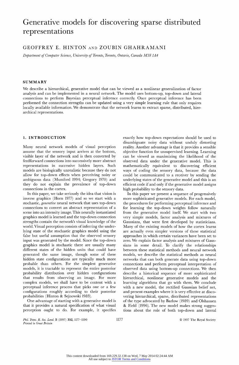
j hidden units

visible units

Figure 1. A generative neural network for mixtures of Gaussians.

connections in the cortex and it also suggests why topographic maps are so prevalent.

2. MIXTURES OF GAUSSIANS

A mixture of Gaussians is a model that describes some real data points in terms of underlying Gaussian clusters. There are three aspects of this model which we shall discuss. First, given parameters that specify the means, variances and mixing proportions of the clusters, the model defines a generative distribution which assigns a probability to any possible data point. Second, given the parameter values and a data point, the perceptual interpretation process infers the posterior probability that the data came from each of the clusters. Third, given a set of observed data points, the learning process adjusts the parameter values to maximize the probability that the generative model would produce the observed data.

Viewed as a neural network, a mixture of Gaussians consists of a layer of visible units whose state vector represents a data point and a layer of hidden units each of which represents a cluster (see figure 1). To generate a data point we first pick one of the hidden units,j, with a probability wj and give it a state sj = 1. All other hidden states are set to 0. The generative weight vector of the hidden unit, gj, represents the mean of a Gaussian cluster. When unitj is activated it sends a top-down input of gji to each visible unit, i. Local, zero-mean, Gaussian noise with variance o tis added to the top-down input to produce a sample from an axis-aligned Gaussian that has meangj and a covariance matrix that has the o-? terms along the diagonal and zero elsewhere. The probability of generating a particular vector of visible states, d with elements di, is therefore

1 (d,-gj ) 2 /2,72 p(d) = E irjfl 2i (1)

Interpreting a data point, d, consists of computing the posterior probability that it was generated from each of the hidden units, assuming that it must have come from one of them. Each hidden unit, j, first computes the probability density of the data point under its Gaussian model:

p(dls, = 1) = e(d i-gjj)2/2o f (2)

These conditional probabilities are then weighted by the mixing proportions, wj, and normalized to give the posterior probability or responsibility of each hidden unit, j, for the data point. By Bayes theorem:

p(sj = l d) - 7rjp(d Isj 1 ) (3) Xkwkp(dlsk = 1)(3

The computation of p(dlsj = 1) in equation (2) can be done very simply by using recognition connections, rij, from the visible to the hidden units. The recognition connections are set equal to the generative connections, rij = gii. The normalization in equation (3) could be done by using direct lateral connections or interneurones to ensure that the total activity in the hidden layer is a constant.

Learning consists of adjusting the generative parameters g, a, 7r so as to maximize the product of the probabilities assigned to all the observed data points by equation (1). An efficient way to perform the learning is to sweep through all the observed data points computing p(sj = 1 Id) for each hidden unit and then to reset all the generative parameters in parallel. Angle brackets are used to denote averages over the training data:

gj(new) = (p (sj = lI d) d)/(p (sj = 1 d)), (4)

0-*2(new) = p (sj = 1 Id) (di -gJ.)/, (5)

wj(new) = (p(sj= lId)). (6)

This is a version of the 'expectation and maximiza- tion' algorithm (Dempster et al. 1977) and is guaranteed to raise the likelihood of the observed data unless it is already at a local optimum. The computation of the posterior probabilities of the hidden states given the data (i.e. perceptual inference) is called the E-step and the updating of the parameters is called the M-step.

Instead of performing an M-step after a full sweep through the data it is possible to use an on-line gradient algorithm that uses the same posterior probabilities of hidden states but updates each generative weight using a version of the delta rule with a learning rate of e:

/g,i = c p (sj = 1 Id) (d - gji). (7)

The k-means algorithm (a form of vector quantization) is the limiting case of a mixture of Gaussians model where the variances are assumed equal and infinitesimal and the rj are assumed equal. Under these assumptions the posterior probabilities in equation (3) go to binary values with p (sj = 1 Id) = 1 for the Gaus- sian whose mean is closest to d and 0 otherwise. Competitive learning algorithms (e.g. Rumelhart & Zipser 1985) can generally be viewed as ways of fitting mixture of Gaussians generative models. They are usually inefficient because they do not use a full M- step and slightly wrong because they pick a single

Phil. Trans. R. Soc. Lond. B (1997)



Generative modelsfordiscoveringsparse distributed representations G. E. Hinton and Z. Ghahramani 1179

winner among the hidden units instead of making the states proportional to the posterior probabilities.

Kohonen's self-organizing maps (Kohonen 1982), Durbin & Willshaw's elastic net (1987), and the generative topographic map (Bishop et al. 1997) are variations of vector quantization or mixture of Gaussian models in which additional constraints are imposed that force neighbouring hidden units to have similar generative weight vectors. These constraints typically lead to a model of the data that is worse when measured by equation (1). So in these models, topographic maps are not a natural consequence of trying to maximize the likelihood of the data. They are imposed on the mixture model to make the solution easier to interpret and more brain-like. By contrast, the algorithm we present later has to produce topographic maps to maximize the data likelihood in a sparsely connected net.

Because the recognition weights are just the transpose of the generative weights and because many researchers do not think in terms of generative models, neural network models that perform competitive learning typically only have the recognition weights required for perceptual inference. The weights are learned by applying the rule that is appropriate for the generative weights. This makes the model much simpler to implement but harder to understand.

Neural net models of unsupervised learning that are derived from mixtures have simple learning rules and produce representations that are a highly nonlinear function of the data, but they suffer from a disastrous weakness in their representational abilities. Each data point is represented by the identity of the winning hidden unit (i.e. the cluster it belongs to). So for the representation to contain, on average, n bits of information about the data, there must be at least 2n hidden units. (This point is often obscured by the fact that the posterior distribution is a vector of real-valued states across the hidden units. This vector contains a lot of information about the data and supervised radial basis function networks make use of this rich information. However, from the generative or coding viewpoint, the posterior distribution must be viewed as a probability distribution across discrete impoverished representations, not a real-valued representation.)

3. FACTOR ANALYSIS

In factor analysis, correlations among observed variables are explained in terms of shared hidden variables called factors which have real-valued states. Viewed as a neural network, the generative model underlying a standard version of factor analysis assumes that the state, yj of each hidden unit, j, is chosen independently from a zero-mean, unit-variance Gaussian and the state, di, of each visible unit, i, is then chosen from a Gaussian with variance oa and mean Ejyjgj.. So the only difference from the mixture of Gaussians model is that the hidden state vectors are continuous and Gaus- sian distributed rather than discrete vectors that contain a single 1.

The probability of generating a particular vector of visible states, d, is obtained by integrating over all

possible states, y, of the hidden units, weighting each hidden state vector by its probability under the generative model:

p (d) P (y)p(dIy)dy (8)

y21 ei/2H 1 (di-Eyjgji)2/2,?dy.

(9)

Because the network is linear and the noise is Gaus- sian, this integral is tractable.

Maximum likelihood factor analysis (Everitt 1984) consists of finding generative weights and local noise levels for the visible units so as to maximize the likelihood of generating the observed data. Without loss of generality, the generative noise model for the hidden units can be set to be a zero mean Gaussian with a covariance equal to the identity matrix.

(a) Computing posterior distributions

Given some generative parameters and an observed data point, the perceptual inference problem is to compute the posterior distribution in the continuous hidden space. This is not as simple as computing the discrete posterior distribution for a mixture of Gaus- sians model. Fortunately, the posterior distribution in the continuous factor space is a Gaussian whose mean depends linearly on the data point and can be computed using recognition connections.

There are several reasons why the correct recognition weights are not, in general, equal to the generative weights. Visible units with lower local noise variances will have larger recognition weights, all else being equal. But even if all the visible noise variances are equal, the recognition weights need not be proportional to the generative weights because the generative weight vectors of the hidden units (known as the factor loadings) do not need to be orthogonal. (If an invertible linear transformation, L, is applied to all the generative weight vectors and L-1 is applied to the prior noise distribution of the hidden units, the likelihood of the data is unaffected. The only consequence is that L-1 gets applied to the posterior distributions in hidden space. This means that the generative weight vectors can always be forced to be orthogonal, but only if a full covariance matrix is used for the prior.) Generative weight vectors that are not orthogonal give rise to a very important phenomenon known as 'explaining away' that occurs during perceptual inference (Pearl 1988).

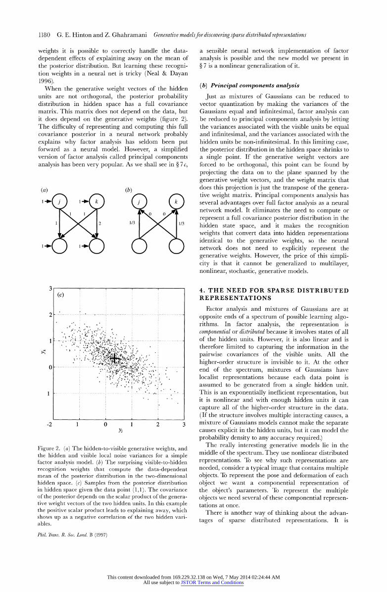
Suppose that the visible units all have equal noise variances and that two hidden units have generative weight vectors that have a positive scalar product. Even though the states of the two hidden units are uncorrelated in the generative model, they will be anti-correlated in the posterior distribution for a given data point. When one of the units is highly active it 'explains' the part of the data point that projects on to it and so there is no need for the other hidden unit to be so active (figure 2). By using appropriate recognition

Phil. Trans. R. Soc. Loand. B (1997)



1180 G. E. Hinton and Z. Ghahramani Generative modeisfordiscoveringsparse distributed representations

weights it is possible to correctly handle the data- dependent effects of explaining away on the mean of the posterior distribution. But learning these recognition weights in a neural net is tricky (Neal & Dayan 1996).

When the generative weight vectors of the hidden units are not orthogonal, the posterior probability distribution in hidden space has a full covariance matrix. This matrix does not depend on the data, but it does depend on the generative weights (figure 2). The difficulty of representing and computing this full covariance posterior in a neural network probably explains why factor analysis has seldom been put forward as a neural model. However, a simplified version of factor analysis called principal components analysis has been very popular. As we shall see in ? 7 c,

a sensible neural network implementation of factor analysis is possible and the new model we present in ? 7 is a nonlinear generalization of it.

(b) Principal components analysis

Just as mixtures of Gaussians can be reduced to vector quantization by making the variances of the Gaussians equal and infinitesimal, factor analysis can be reduced to principal components analysis by letting the variances associated with the visible units be equal and infinitesimal, and the variances associated with the hidden units be non-infinitesimal. In this limiting case, the posterior distribution in the hidden space shrinks to a single point. If the generative weight vectors are forced to be orthogonal, this point can be found by projecting the data on to the plane spanned by the generative weight vectors, and the weight matrix that does this projection is just the transpose of the generative weight matrix. Principal components analysis has several advantages over full factor analysis as a neural network model. It eliminates the need to compute or represent a full covariance posterior distribution in the hidden state space, and it makes the recognition weights that convert data into hidden representations identical to the generative weights, so the neural network does not need to explicitly represent the generative weights. However, the price of this simplicity is that it cannot be generalized to multilayer, nonlinear, stochastic, generative models.

4. THE NEED FOR SPARSE DISTRIBUTED REPRESENTATIONS

Factor analysis and mixtures of Gaussians are at opposite ends of a spectrum of possible learning algorithms. In factor analysis, the representation is componential or distributed because it involves states of all of the hidden units. However, it is also linear and is therefore limited to capturing the information in the pairwise covariances of the visible units. All the higher-order structure is invisible to it. At the other end of the spectrum, mixtures of Gaussians have localist representations because each data point is assumed to be generated from a single hidden unit. This is an exponentially inefficient representation, but it is nonlinear and with enough hidden units it can capture all of the higher-order structure in the data. (If the structure involves multiple interacting causes, a mixture of Gaussians models cannot make the separate causes explicit in the hidden units, but it can model the probability density to any accuracy required.)

The really interesting generative models lie in the middle of the spectrum. They use nonlinear distributed representations. To see why such representations are needed, consider a typical image that contains multiple objects. To represent the pose and deformation of each object we want a componential representation of the object's parameters. To represent the multiple objects we need several of these componential representations at once.

There is another way of thinking about the advantages of sparse distributed representations. It is

(a) (b)

14 14

0 0

1 v 2 1/3 1/3

3 (c)

2 .. . . . . . . . . . ......;

1 ............................... . . . . . . . . . . . . . ... . . . . . . . . . . . . . ............ .. . ........

-2 1 0 1 2 3 YJ

Figure 2. (a) The hidden-to-visible generative weights, and the hidden and visible local noise variances for a simple factor analysis model. (b) The surprising visible-to-hidden recognition weights that compute the data-dependent mean of the posterior distribution in the two-dimensional hidden space. (c) Samples from the posterior distribution in hidden space given the data point (1,1). The covariance of the posterior depends on the scalar product of the generative weight vectors of the two hidden units. In this example the positive scalar product leads to explaining away, which shows up as a negative correlation of the two hidden variables.




Generative modelsfor discovering sparse distributed representations G. E. Hinton and Z. Ghahramani 1181

advantageous to represent images in terms of basis functions (as factor analysis does), but for different classes of images, different basis functions are appropriate. So it is useful to have a large repertoire of basis functions and to select the subset that are optimal for representing the current image.

If an efficient algorithm can be found for fitting models of this type it is likely to prove even more fruitful than the efficient back-propagation algorithm for multilayer nonlinear regression (Rumelhart et al. 1986). The difficulty lies in the computation of the posterior distribution over hidden states when given a data point. This distribution, or an approximation to it, is required both for learning the generative model and for perceptual inference once the model has been learned. Mixtures of Gaussians and factor analysis are standard statistical models precisely because the exact computation of the posterior distribution is tractable.

5. FROM BOLTZMANN MACHINES TO LOGISTIC BELIEF NETS

The Boltzmann machine (Hinton & Sejnowski 1986) was, perhaps, the first neural network learning algorithm to be based on an explicit generative model that used distributed, nonlinear representations. Boltzmann machines use stochastic binary units and, with h hidden units, the number of possible representations of each data point is 2h. It would take exponential time to compute the posterior distribution across all of these possible representations and most of them would typically have probabilities very close to 0, so the Boltzmann machine uses a Monte-Carlo method known as Gibbs sampling (Hinton & Sejnowski 1983; Geman & Geman 1984) to pick stochastically representations according to their posterior probabilities. Both the Gibbs sampling for perceptual inference and the learning rule for following the gradient of the log likelihood of the data are remarkably simple to implement in a network of symmetrically connected stochastic binary units. Unfortunately, the learning algorithm is extremely slow and, as a result, the unsupervised form of the algorithm never really succeeded in extracting interesting hierarchical representations.

The Boltzmann machine learning algorithm is slow for two reasons. First, the perceptual inference is slow because it must spend a long time doing Gibbs sampling before the probabilities are correct. Second, the learning signal for the weight between two units is the dilference between their sampled correlation in two different conditions. When the two correlations are similar, the sampling noise makes their difference extremely noisy.

Neal (1992) realized that learning is considerably more efficient if, instead of symmetric connections, the generative model uses directed connections that form an acyclic graph. This kind of generative model is called a belief network and it has an important prop- erty that is missing in models whose generative connections form cycles: it is straightforward to compute the joint probability of a data point and a configuration of states of all the hidden units. In a Boltzmann machine, this probability depends not only

on the particular hidden states but also on an additional normalization term called the partition function that involves all possible configurations of states. It is the derivatives of the partition function that make Boltz- mann machine learning so inefficient.

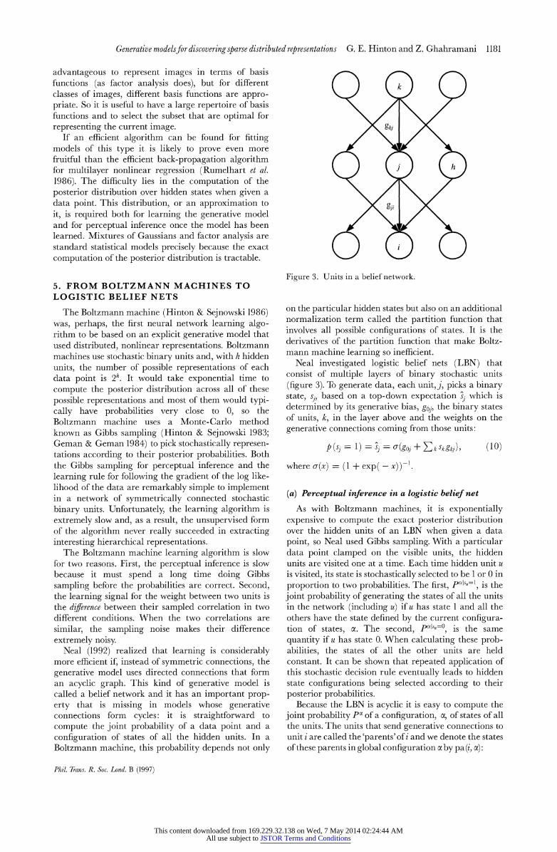
Neal investigated logistic belief nets (LBN) that consist of multiple layers of binary stochastic units (figure 3). To generate data, each unit,j, picks a binary state, sj, based on a top-down expectation sj which is determined by its generative bias, goj, the binary states of units, k, in the layer above and the weights on the generative connections coming from those units:

P(si = 1) =s = (9g0+ ?kSkgkj), (10)

where v(x) = (1 + exp( -x))-.

(a) Perceptual inference in a logistic belief net

As with Boltzmann machines, it is exponentially expensive to compute the exact posterior distribution over the hidden units of an LBN when given a data point, so Neal used Gibbs sampling. With a particular data point clamped on the visible units, the hidden units are visited one at a time. Each time hidden unit u is visited, its state is stochastically selected to be 1 or 0 in proportion to two probabilities. The first, PcIsu=l, is the joint probability of generating the states of all the units in the network (including u) if u has state 1 and all the others have the state defined by the current configuration of states, oa. The second, pals,=?, is the same quantity if u has state 0. When calculating these probabilities, the states of all the other units are held constant. It can be shown that repeated application of this stochastic decision rule eventually leads to hidden state configurations being selected according to their posterior probabilities.

Because the LBN is acyclic it is easy to compute the joint probability Pa of a configuration, oc of states of all the units. The units that send generative connections to unit i are called the 'parents' of i and we denote the states of these parents in global configuration a by pa (i, a):

Figure 3. Units in a belief network.




1182 G. E. Hinton and Z. Ghahramani Generativemodelsfordiscoveringsparsedistributed representations

P= a

P (sVIpa(i, a)), (11)

where sa is the binary state of unit i in configuration oa. It is convenient to work in the domain of negative log

probabilities which are called energies by analogy with statistical physics. We define Ea to be -ln Pa,

E1 =a - (salnsa + (1 - sa)ln(l - S)) (12) u

where sa is the binary state of unit u in configuration oa, us is the top-down expectation generated by the layer above, and u is an index over all the units in the net.

The rule for stochastically picking a new state for u requires the ratio of two probabilities and hence the difference of two energies

AEa = Ea1su=0 - Ealsu=l, (13)

p (su = 1Ucl) = a(AEa). (14)

All the contributions to the energy of configuration a that do not depend on sj can be ignored when computing AEj. This leaves a contribution that depends on the top-down expectation sj generated by the units in the layer above (see equation (10)) and a contribution that depends on both the states, si and the top-down expectations, Si, of units in the layer below (figure 3)

AEja= ln -ln(1- )

+E [sa lI1 - n(l - Sa

oals.-O oals.=O -s?Ilns + (1- sa)ln(1 -s S (15

Given samples from the posterior distribution, the generative weights of a LBN can be learned by using the on-line delta rule which performs gradient ascent in the log likelihood of the data:

Agji = csj (Si - Si). (16)

Until very recently (Lewicki & Sejnowski 1997), logistic belief nets were widely ignored as models of neural computation. This may be because the computation of AEa in equation (15) requires unitj to observe not only the states of units in the layer below but also their top-down expectations. In ? 7 c we show how this problem can be finessed but first we describe an alternative way of making LBNs biologically plausible.

6. THE WAKE-SLEEP ALGORITHM

There is an approximate method of performing perceptual inference in a LBN that leads to a very simple implementation which would be biologically quite plausible if only it were better at extracting the hidden causes of data (Hinton et al. 1995). Instead of using Gibbs sampling, we use a separate set of bottom- up recognition connections to pick binary states for units in one layer given the already selected binary states of units in the layer below. The learning rule for the top-down generative weights is the same as for an LBN. It can be shown that this learning rule, instead of following the gradient of the log likelihood now

follows the gradient of the penalized log likelihood where the penalty term is the Kullback-Liebler diver- gence between the true posterior distribution and the distribution produced by the recognition connections. The penalized log likelihood acts as a lower bound on the log likelihood of the data and the effect of learning is to improve this lower bound. In attempting to raise the bound, the learning tries to adjust the generative model so that the true posterior distribution is as close as possible to the distribution actually computed by the recognition weights.

The recognition weights are learned by introducing a 'sleep' phase in which the generative model is run top- down to produce fantasy data. The network knows the true hidden causes of the fantasy data and the recognition connections are adjusted to maximize the likelihood of recovering these causes. This is just a simple application of the delta rule where the learning signal is obtained by comparing the probability that the recognition connections would turn a unit on with the state it actually had when the fantasy data was generated.

The attractive properties of the wake-sleep algorithm are that the perceptual inference is simple and fast, and the learning rules for the generative and recognition weights are simple and entirely local. Unfortunately it has some serious disadvantages.

(i) The recognition process does not do correct probabilistic inference based on the generative model. It does not handle explaining away in a principled manner and it does not allow for top-down effects in perception.

(ii) The sleep phase of the learning algorithm only approximately follows the gradient of the penalized log likelihood.

(iii) Continuous quantities such as intensities, dis- tances or orientations have to be represented using stochastic binary neurones, which is inefficient.

(iv) Although the learning algorithm works reason- ably well for some tasks, considerable parameter- tweaking is necessary to get it to produce easily interpretable hidden units on toy tasks such as the one described in ? 8. On other tasks, such as the one described in ? 9, it consistently fails to capture obvious hidden structure. This is probably because of its inabil- ity to handle explaining away correctly.

7. RECTIFIED GAUSSIAN BELIEF NETS

We now describe a new model called the rectified Gaussian belief net (RGBN) which seems to work much better than the wake-sleep algorithm. The RGBN uses units with states that are either positive real values or zero, so it can represent real-valued latent variables directly. Its main disadvantage is that the recognition process involves Gibbs sampling which could be very time consuming. In practice, however, ten to 20 samples per unit have proved adequate for some small but interesting tasks.

We first describe the RGBN without considering neural plausibility. Then we show how lateral interactions within a layer can be used to perform explaining away correctly. This makes the RGBN far





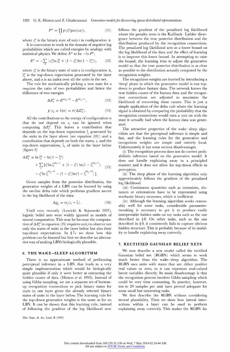
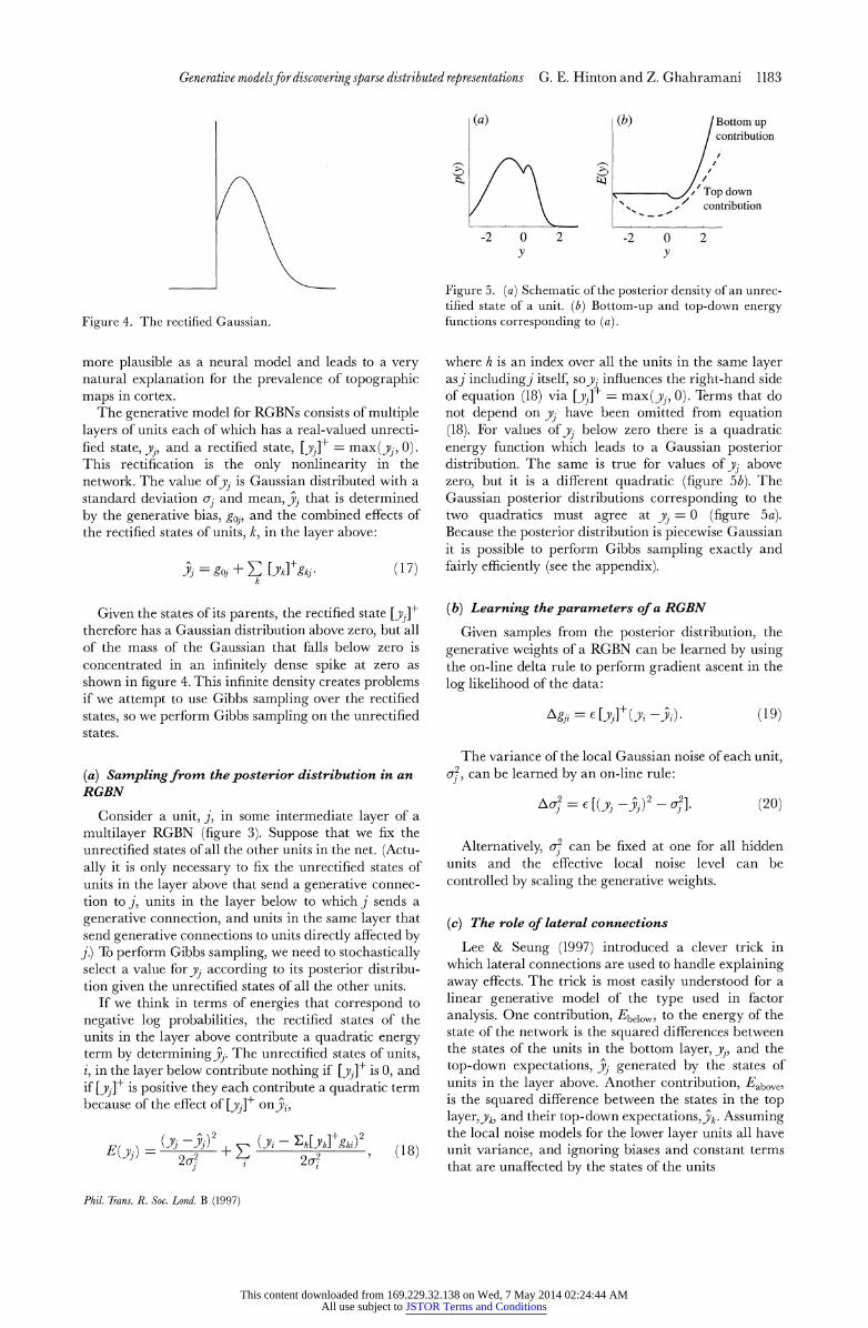
Figure 4. The rectified Gaussian.

more plausible as a neural model and leads to a very natural explanation for the prevalence of topographic maps in cortex.

The generative model for RGBNs consists of multiple layers of units each of which has a real-valued unrectified state, yj, and a rectified state, [yj]+ = max(yj, 0). This rectification is the only nonlinearity in the network. The value ofyj is Gaussian distributed with a standard deviation oj and mean, yj that is determined by the generative bias, goj, and the combined effects of the rectified states of units, k, in the layer above:

Yi Igi+ E [Yk]gkj- (17) k

Given the states of its parents, the rectified state [yj]+ therefore has a Gaussian distribution above zero, but all of the mass of the Gaussian that falls below zero is concentrated in an infinitely dense spike at zero as shown in figure 4. This infinite density creates problems if we attempt to use Gibbs sampling over the rectified states, so we perform Gibbs sampling on the unrectified states.

(a) Sampling from the posterior distribution in an RGBN

Consider a unit, j, in some intermediate layer of a multilayer RGBN (figure 3). Suppose that we fix the unrectified states of all the other units in the net. (Actu- ally it is only necessary to fix the unrectified states of units in the layer above that send a generative connection to j, units in the layer below to which j sends a generative connection, and units in the same layer that send generative connections to units directly affected by j.) To perform Gibbs sampling, we need to stochastically select a value foryj according to its posterior distribution given the unrectified states of all the other units.

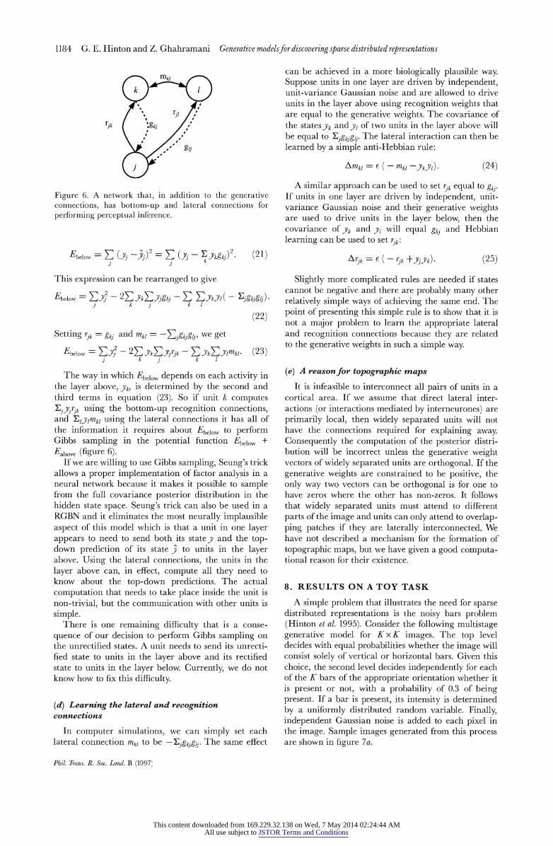
If we think in terms of energies that correspond to negative log probabilities, the rectified states of the units in the layer above contribute a quadratic energy term by determining 3. The unrectified states of units, i, in the layer below contribute nothing if [y1] is 0, and if [yj]+ is positive they each contribute a quadratic term because of the effect of [yi]? onyr,

E( ( Yi ( i ) (> -i EhL[Yh]ghi)

(a) (b) Bottom up contribution

SI/4 > \ Top down 7'contribution

-2 0 2 -2 0 2 y y

Figure 5. (a) Schematic of the posterior density of an unrectified state of a unit. (b) Bottom-up and top-down energy functions corresponding to (a).

where h is an index over all the units in the same layer asj includingj itself, soyj influences the right-hand side of equation (18) via [yj]+ = max(yj, 0). Terms that do not depend on yj have been omitted from equation (18). For values of%y below zero there is a quadratic energy function which leads to a Gaussian posterior distribution. The same is true for values of yi above zero, but it is a different quadratic (figure 5b). The Gaussian posterior distributions corresponding to the two quadratics must agree at yj = 0 (figure 5a). Because the posterior distribution is piecewise Gaussian it is possible to perform Gibbs sampling exactly and fairly efficiently (see the appendix).

(b) Learning the parameters of a RGBN

Given samples from the posterior distribution, the generative weights of a RGBN can be learned by using the on-line delta rule to perform gradient ascent in the log likelihood of the data:

i\gjil = 6[Yj1 (Yi -Y^I) (19)

The variance of the local Gaussian noise of each unit, ?, can be learned by an on-line rule:

= e [ 2 )2 _ (20)

Alternatively, ? can be fixed at one for all hidden units and the effective local noise level can be controlled by scaling the generative weights.

(c) The role of lateral connections

Lee & Seung (1997) introduced a clever trick in which lateral connections are used to handle explaining away effects. The trick is most easily understood for a linear generative model of the type used in factor analysis. One contribution, Ebelow) to the energy of the state of the network is the squared differences between the states of the units in the bottom layer, yj, and the top-down expectations, yjj generated by the states of units in the layer above. Another contribution, Eabove) is the squared difference between the states in the top layer,yk, and their top-down expectations,3k. Assuming the local noise models for the lower layer units all have unit variance, and ignoring biases and constant terms that are unaffiected by the states of the units




1184 G. E. Hinton and Z. Ghahramani Generative modelsfordiscovering sparse distributed representations

Mkl

/ sss ~~~rj ,, rJk '(gkj /

Figure 6. A network that, in addition to the generative connections, has bottom-up and lateral connections for performing perceptual inference.

Ebelow = Z (Y; ) = Z (YJi - Y.YkgkJ)' (21)

This expression can be rearranged to give

Ebelow = E - -2EYkEYjgkj - E EYkYl( -

Ejgkjglj)- j k j k I

(22)

Setting rjk = gkj and mkl =-Ejgkjglj, we get

Ebelow = E - 2EYkEYjrjk - EYkEYlnmkl- (23) j k j k I

The way in which Ebelow depends on each activity in the layer above, Yk, is determined by the second and third terms in equation (23). So if unit k computes EjyjJrjk using the bottom-up recognition connections, and XIylmkl using the lateral connections it has all of the information it requires about Eb,10w to perform Gibbs sampling in the potential function Eb1jow + Eabove (figure 6).

If we are willing to use Gibbs sampling, Seung's trick allows a proper implementation of factor analysis in a neural network because it makes it possible to sample from the full covariance posterior distribution in the hidden state space. Seung's trick can also be used in a RGBN and it eliminates the most neurally implausible aspect of this model which is that a unit in one layer appears to need to send both its statey and the top- down prediction of its state y to units in the layer above. Using the lateral connections, the units in the layer above can, in effect, compute all they need to know about the top-down predictions. The actual computation that needs to take place inside the unit is non-trivial, but the communication with other units is simple.

There is one remaining difficulty that is a consequence of our decision to perform Gibbs sampling on the unrectified states. A unit needs to send its unrectified state to units in the layer above and its rectified state to units in the layer below. Currently, we do not know how to fix this difficulty.

(d) Learning the lateral and recognition connections

In computer simulations, we can simply set each lateral connection mkl to be -Ejgkjglj. The same effect

Phil. Trans. R. Soc. Lond. B (1997'

can be achieved in a more biologically plausible way. Suppose units in one layer are driven by independent, unit-variance Gaussian noise and are allowed to drive units in the layer above using recognition weights that are equal to the generative weights. The covariance of the statesYk andy, of two units in the layer above will be equal to Ejgkjglj. The lateral interaction can then be learned by a simple anti-Hebbian rule:

A mkl = E ( - mkl -YkY1) (24)

A similar approach can be used to set rjk equal to gkj. If units in one layer are driven by independent, unit- variance Gaussian noise and their generative weights are used to drive units in the layer below, then the covariance Of Yk and yi will equal gkj and Hebbian learning can be used to set rjk:

Ar,k = e (-rJk +YJYk) (25)

Slightly more complicated rules are needed if states cannot be negative and there are probably many other relatively simple ways of achieving the same end. The point of presenting this simple rule is to show that it is not a major problem to learn the appropriate lateral and recognition connections because they are related to the generative weights in such a simple way.

(e) A reason for topographic maps

It is infeasible to interconnect all pairs of units in a cortical area. If we assume that direct lateral interactions (or interactions mediated by interneurones) are primarily local, then widely separated units will not have the connections required for explaining away. Consequently the computation of the posterior distribution will be incorrect unless the generative weight vectors of widely separated units are orthogonal. If the generative weights are constrained to be positive, the only way two vectors can be orthogonal is for one to have zeros where the other has non-zeros. It follows that widely separated units must attend to different parts of the image and units can only attend to overlap- ping patches if they are laterally interconnected. We have not described a mechanism for the formation of topographic maps, but we have given a good computa- tional reason for their existence.

8. RESULTS ON A TOY TASK

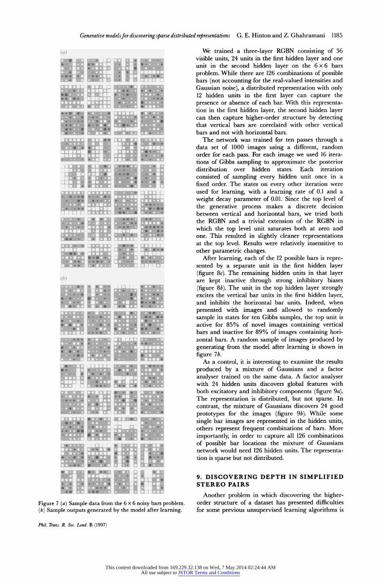
A simple problem that illustrates the need for sparse distributed representations is the noisy bars problem (Hinton et al. 1995). Consider the following multistage generative model for K x K images. The top level decides with equal probabilities whether the image will consist solely of vertical or horizontal bars. Given this choice, the second level decides independently for each of the K bars of the appropriate orientation whether it is present or not, with a probability of 0.3 of being present. If a bar is present, its intensity is determined by a uniformly distributed random variable. Finally, independent Gaussian noise is added to each pixel in the image. Sample images generated from this process are shown in figure 7a.



Generative modelsfordiscoveringsparse distributed representations G. E. Hinton and Z. Ghahramani 1185

(a) U -''.H U,, U,,.[ U.,, _[Eh1---r U,.,i 1 U,., i U,..[ (b)I_ U,., _ U,,, U,., U,., U,, U, E m:-s -ia ~~L H,-Li J

Fiue7()Smle aafo h nis bas rblm (b Sapeotusgnrtdb h oe fe erig

We trained a three-layer RGBN consisting of 36 visible units, 24 units in the first hidden layer and one unit in the second hidden layer on the 6 x 6 bars problem. While there are 126 combinations of possible bars (not accounting for the real-valued intensities and Gaussian noise), a distributed representation with only 12 hidden units in the first layer can capture the presence or absence of each bar. With this representation in the first hidden layer, the second hidden layer can then capture higher-order structure by detecting that vertical bars are correlated with other vertical bars and not with horizontal bars.

The network was trained for ten passes through a data set of 1000 images using a different, random order for each pass. For each image we used 16 iterations of Gibbs sampling to approximate the posterior distribution over hidden states. Each iteration consisted of sampling every hidden unit once in a fixed order. The states on every other iteration were used for learning, with a learning rate of 0.1 and a weight decay parameter of 0.01. Since the top level of the generative process makes a discrete decision between vertical and horizontal bars, we tried both the RGBN and a trivial extension of the RGBN in which the top level unit saturates both at zero and one. This resulted in slightly cleaner representations at the top level. Results were relatively insensitive to other parametric changes.

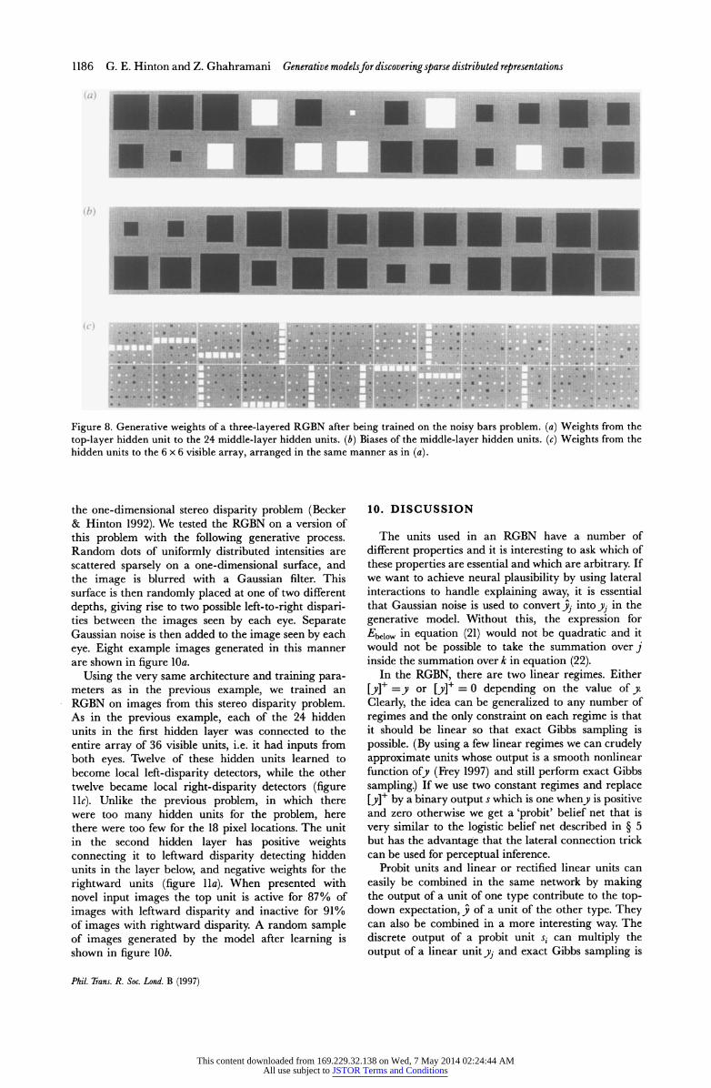
After learning, each of the 12 possible bars is represented by a separate unit in the first hidden layer (figure 8c). The remaining hidden units in that layer are kept inactive through strong inhibitory biases (figure 8b). The unit in the top hidden layer strongly excites the vertical bar units in the first hidden layer, and inhibits the horizontal bar units. Indeed, when presented with images and allowed to randomly sample its states for ten Gibbs samples, the top unit is active for 85% of novel images containing vertical bars and inactive for 89% of images containing horizontal bars. A random sample of images produced by generating from the model after learning is shown in figure 7b.

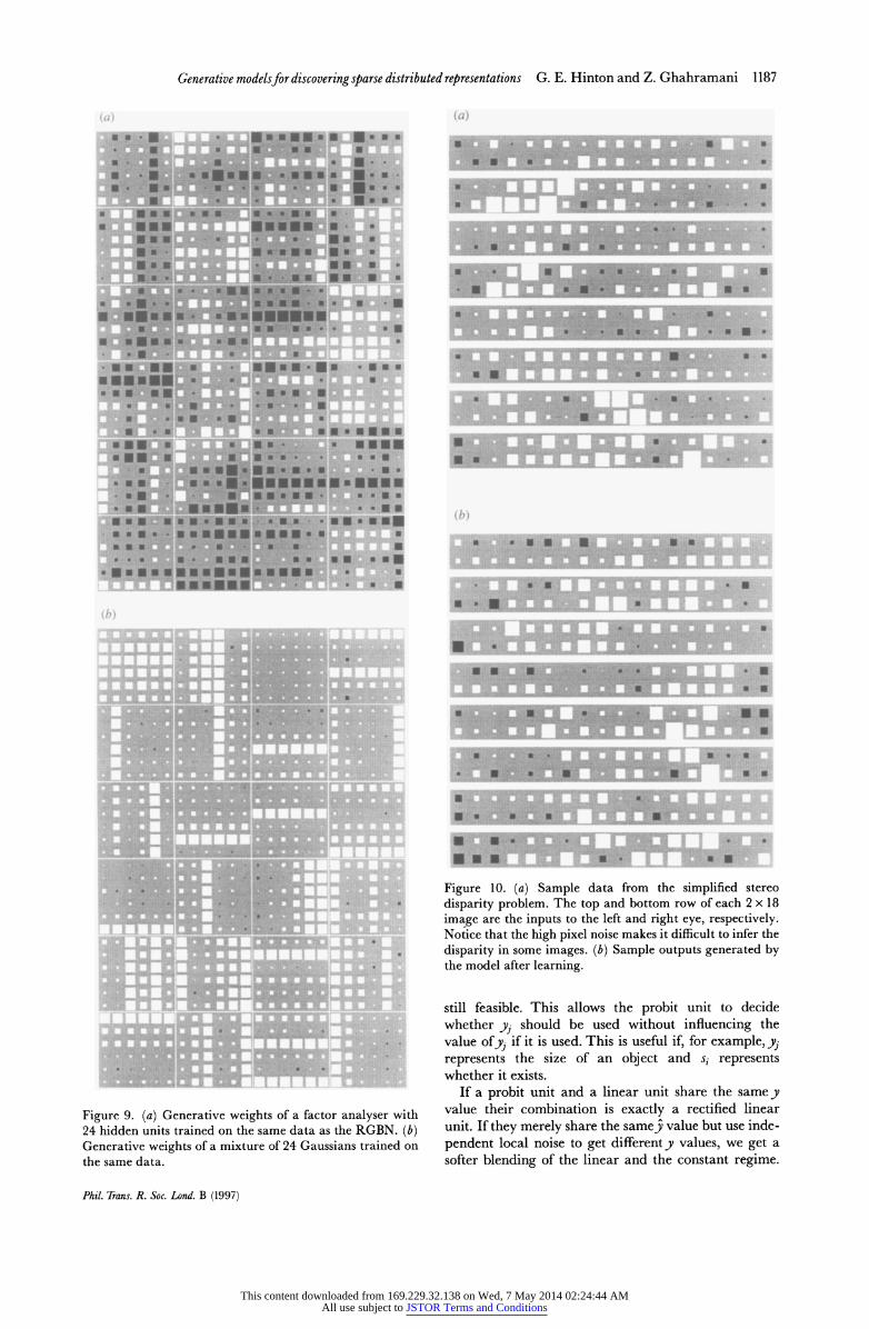
As a control, it is interesting to examine the results produced by a mixture of Gaussians and a factor analyser trained on the same data. A factor analyser with 24 hidden units discovers global features with both excitatory and inhibitory components (figure 9a). The representation is distributed, but not sparse. In contrast, the mixture of Gaussians discovers 24 good prototypes for the images (figure 9b). While some single bar images are represented in the hidden units, others represent frequent combinations of bars. More importantly, in order to capture all 126 combinations of possible bar locations the mixture of Gaussians network would need 126 hidden units. The representation is sparse but not distributed.

9. DISCOVERING DEPTH IN SIMPLIFIED STEREO PAIRS

Another problem in which discovering the higher- order structure of a dataset has presented difficulties for some previous unsupervised learning algorithms is




1186 G. E. Hinton and Z. Ghahramani Generative modelsfor discoveringsparse distributed representations

( r)r~ ~~~~~~~~~~~~~~~~~~~~~~~~~~~~~~~~~~~~~~~~~~~~~~~ M I I - . M M

(b)

.~~~~~~~ % 8 .. ~ ~ ~ ~ ~ ~ .. . . .. . .. . .

cE

*S.~ ~ ~ ~ ~ ~ ~ ~ ~ ~ ~~~~~~~:l E .

,., : ............. .........A.' .. . -

Figure 8. Generative weights of a three-layered RGBN after being trained on the noisy bars problem. (a) Weights from the top-layer hidden unit to the 24 middle-layer hidden units. (b) Biases of the middle-layer hidden units. (c) Weights from the hidden units to the 6 x 6 visible array, arranged in the same manner as in (a).

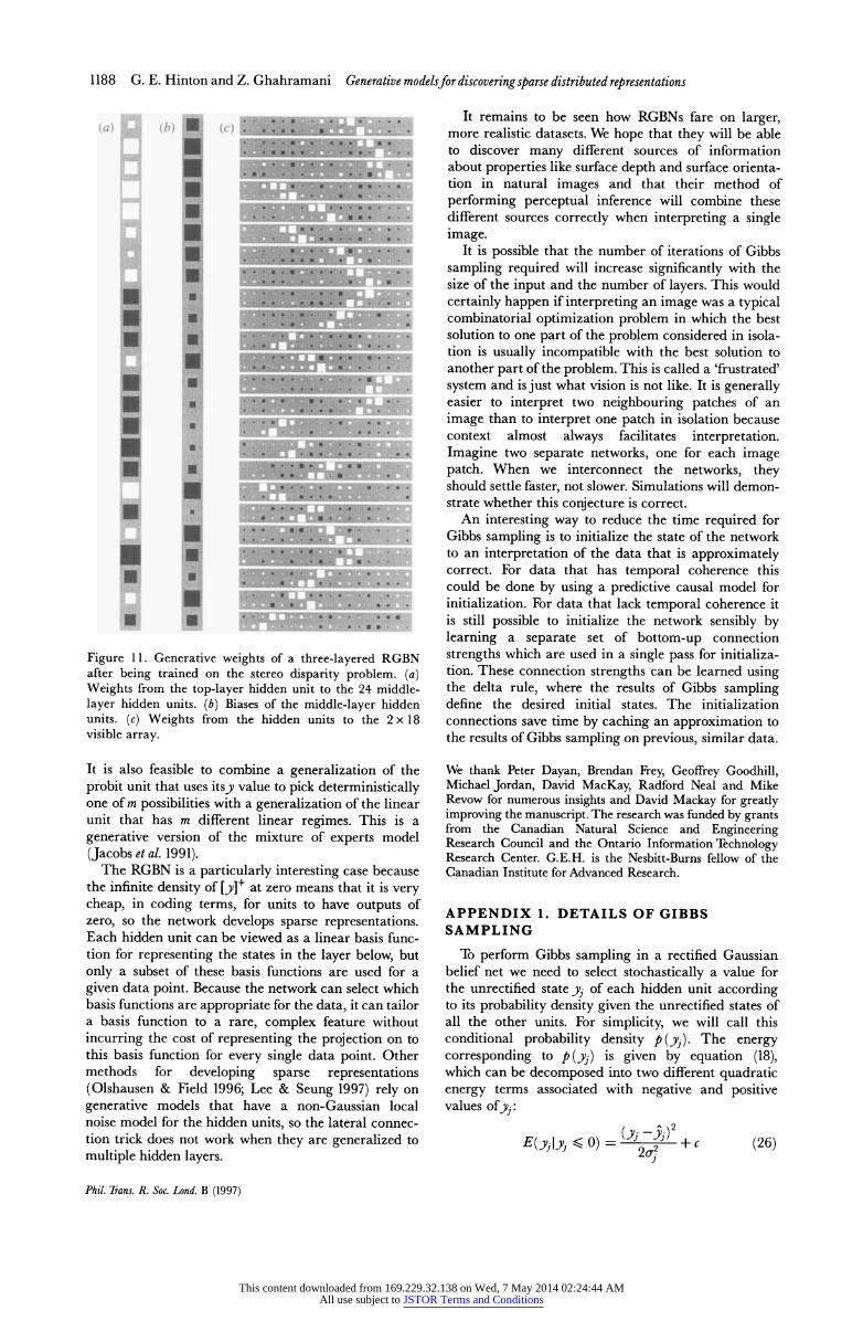
the one-dimensional stereo disparity problem (Becker & Hinton 1992). We tested the RGBN on a version of this problem with the following generative process. Random dots of uniformly distributed intensities are scattered sparsely on a one-dimensional surface, and the image is blurred with a Gaussian filter. This surface is then randomly placed at one of two different depths, giving rise to two possible left-to-right dispari- ties between the images seen by each eye. Separate Gaussian noise is then added to the image seen by each eye. Eight example images generated in this manner are shown in figure lOa.

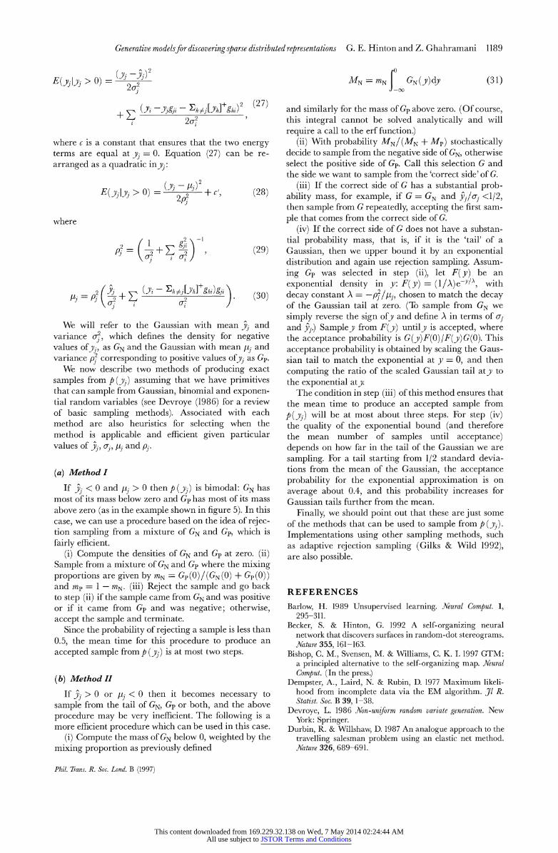
Using the very same architecture and training parameters as in the previous example, we trained an RGBN on images from this stereo disparity problem. As in the previous example, each of the 24 hidden units in the first hidden layer was connected to the entire array of 36 visible units, i.e. it had inputs from both eyes. Twelve of these hidden units learned to become local left-disparity detectors, while the other twelve became local right-disparity detectors (figure 1 lc). Unlike the previous problem, in which there were too many hidden units for the problem, here there were too few for the 18 pixel locations. The unit in the second hidden layer has positive weights connecting it to leftward disparity detecting hidden units in the layer below, and negative weights for the rightward units (figure lla). When presented with novel input images the top unit is active for 87% of images with leftward disparity and inactive for 91% of images with rightward disparity. A random sample of images generated by the model after learning is shown in figure lOb.

10. DISCUSSION

The units used in an RGBN have a number of different properties and it is interesting to ask which of these properties are essential and which are arbitrary. If we want to achieve neural plausibility by using lateral interactions to handle explaining away, it is essential that Gaussian noise is used to convert j into yj in the generative model. Without this, the expression for Ebe,ow in equation (21) would not be quadratic and it would not be possible to take the summation over j inside the summation over k in equation (22).

In the RGBN, there are two linear regimes. Either [y]+ =y or [y]+ = 0 depending on the value of y. Clearly, the idea can be generalized to any number of regimes and the only constraint on each regime is that it should be linear so that exact Gibbs sampling is possible. (By using a few linear regimes we can crudely approximate units whose output is a smooth nonlinear function ofy (Frey 1997) and still perform exact Gibbs sampling.) If we use two constant regimes and replace [y]+ by a binary output s which is one wheny is positive and zero otherwise we get a 'probit' belief net that is very similar to the logistic belief net described in ? 5 but has the advantage that the lateral connection trick can be used for perceptual inference.

Probit units and linear or rectified linear units can easily be combined in the same network by making the output of a unit of one type contribute to the top- down expectation, y of a unit of the other type. They can also be combined in a more interesting way. The discrete output of a probit unit si can multiply the output of a linear unityj and exact Gibbs sampling is




Generative modelsfor discovering sparse distributed representations G.E.Hintonand Z.Ghahramani 1187

(cZ) .- .;0 2 fi _ s3 > e X -_ S B S ____E r 0 B l _ EZ [' g I li#S fi 3E |M a l ! 1- N lL &g | I 1 | S 111S1 11|1 11S1____ r38 BE i U SIB F gi r t | . w S _ R ff ? SV 8 l ^ . - . : i I . K _ I i - -?

? | | I I E F lP - R | , B B | R I - i | | | | | | li " " | l - | | | ^ 8^- -i v I | _-t-11 2s l I -E _ 1 - -_ Le 111 | 01 l 3 -lli l# E 1E1 | l | B 1 _|__ BIB SE N I g - ._ _ s i lill E _ . - _ __

L | I I | | | . L L | l | | | | L P - S S " . - .-r - | l P | - r _ F . _ S EL: I I --- ILs fi FlllS fi Xw ixw s | | - - - - | l _ - | | - > _ ES _L_ a S iu

X ___?E.<vgEljE _r_r [ 6. 6 6.S

_--___>SA?| *3a_--_g g s S Ej,BS __ ______J a . S N ->S

...l , t: Eaas_ t

x _}T_ g B l _

- __T___ ___ __ _- __? l g U ZLM

-- . ' sX_E ___ . , _S s s SE Sver<ig,kg-

S-r s l- g [; ;+vA=2

_e___ __|_nrB - - - 'EBZ s i

- - - 1 :? ? Z - [ - s@ Z B tL L ^

>"^Rm

J *>sa__ _= C __

_ $ l ..s

bE____ ., K_

. _____ _ ______

.__

_ 2#: ___ ?_ _ S_X_ ___ _____ _ E__ X 3 S 3BE ss

S: ___

____ ____ we _

__Y. v-

-E g _Ra____e3 *_----e3_

s-X a-- :___! w__-____ t sfi efi ss e B 2_? s3eSvM v ERmi4*fi____ ___s

)

.' - - " l;.,_J _ ! Yqmm WX--- ._S i l_ _ | rT.$ S,E

xA g B B B S R g 5g E t> !

gV= ^ 3 ie,bS2ws s r 5]E 23? Y?j_? Q

-____P

_-b_ SK _-''''sSIB _P_3XE_

|, _a _tvvM 'l ,E to_ _ __, ;,ez-c

e X- 'g_>'>X4;e tex"BK w 51 - Ng _WS lg $ F B t rS, ;;=lXv gg2

8?SME: 1 L v8 E

W_|W__ * \ .

e3i4R _ll-__Bff $ ,E3__z9 tS:-S a stl.. _X4|_ gmws ____oox _ _xbe ED _ ,,; S,gg gNS, ->3g B. .SS eE --;*XS - xf

S;> RE E.s

@_________

e _ R_ 3g_gi

#U } _K.i E= ;E l5 8

__r! . t>rjass,PRjstiEsx- j j j j

vl>.X.s|2>JR$2<Xls4t eiE

H9S * w29YxxeQi3Ssl; xsS8. - ...XIYC tEv%.ig D BE _B _ vWc ,ex i> S-S:x,,<Rv^-' ...................................... '$xv .'S2: x#F:|.-,e,: _ _ _ |- - tS S'XSiBi>A-<2,2ES,2.,,;Sz

s<;Ex

__ , S

_gE l $ - C sS

_ H 2 *2 * s x cx 2 g .u i__-_E1_.vS :v 5 AVt' 'N'x? XS . < gcA

;>tS.2 S "R. Xi vUg'S X.wF c B S! 31 8 BLx S # SE E ^SWA >'fA s2STvs { 'dAfE. - [_V^_J 3R_ _ R 9; Wassyt

X' >:W"A '^ ' ''-t f AV_ _ ='X V>TXV>t' ' >;t V IZ

|+9l * | |J-Xi5gi

_g ? %s-_ W iX s8Sh jgE3 6 oxc '5ig 1:g

4R ge,l ,_LiCh';X

_.n^ tTT=

R R 'iR. Y l_: ._fi;SB rrrrrn ___fs8_

5g __l EG - _X s |* rg

* vStt.Y^E.

IL.lLAt lX t..E...e

Figure 9. (a) Generative weights of a factor analyser with 24 hidden units trained on the same data as the RGBN. (b) Generative weights of a mixture of 24 Gaussians trained on the same data.

(a)

-' E l - - I~~~~~~~~~~~~~~~~~~~~~~~~~~~~~~~~~~~~~----------

iLLL

s 1E | I i I 11

..~~~~~....... -- -- -- i -- - - -- - - --- - -

9 sa --_--------_ ---B'

Figure 1 0. (a) Sample data from the simplified stereo disparity problem. The top and bottom row of each 2 x 18 ima~ge are the inputs to the left and right eye, respectively. Notice that the high pixel noise makes it difficult to infer the disparity in some images. (b) Sample outputs generated by the model after learning.

still feasible. This allows the probit unit to decide whether yj should be used without influencing the value ofyj if it is used. This is useful if, for example, yj represents the size of an object and si represents whether it exists.

If a probit unit and a linear unit share the same y value their combination is exactly a rectified linear unit. If they merely share the samey' value but use independent local noise to get differenty values, we get a softer blending of the linear and the constant regime.




1188 G. E. Hinton and Z. Ghahramani Generative modelsfordiscoveringsparse distributed representations

------------- " - - 3~~~~~~~~~~-------g-

= ~ ~ ~ ~ ~~. ---------- ---------- -- -------- - - - - - - - - - - - - - - - - - - - - - - - - - - -

- - - - - - - -- - - - - -

-------------------- --------

-- -- -- -- - -- -- -- - m ------------------------ ~ ~ ~ ~ -

----------- - -------------

FiueI eeaiewiht fatrelyrdRB after being trained on the stereo disparity problem. (a)~~~~~~~~~~~~~~~~~~~~~~~~~~~~~~~~~~l

W 1Eigt frm the to-ae idnui ote2 ide laer idnuis b isso h idelyrhde

units (c Wegt fo h hde nist he2x1 visile aray

It is also feasible to combine a generalization of the probit unit that uses itsy value to pick deterministically one of m possibilities with a generalization of the linear unit that has m different linear regimes. This is a generative version of the mixture of experts model (Jacobs et al. 1991).

The RGBN is a particularly interesting case because the infinite density of [y]+ at zero means that it is very cheap, in coding terms, for units to have outputs of zero, so the network develops sparse representations. Each hidden unit can be viewed as a linear basis function for representing the states in the layer below, but only a subset of these basis functions are used for a given data point. Because the network can select which basis functions are appropriate for the data, it can tailor a basis function to a rare, complex feature without incurring the cost of representing the projection on to this basis function for every single data point. Other methods for developing sparse representations (Olshausen & Field 1996; Lee & Seung 1997) rely on generative models that have a non-Gaussian local noise model for the hidden units, so the lateral connection trick does not work when they are generalized to multiple hidden layers.

It remains to be seen how RGBNs fare on larger, more realistic datasets. We hope that they will be able to discover many different sources of information about properties like surface depth and surface orientation in natural images and that their method of performing perceptual inference will combine these different sources correctly when interpreting a single image.

It is possible that the number of iterations of Gibbs sampling required will increase significantly with the size of the input and the number of layers. This would certainly happen if interpreting an image was a typical combinatorial optimization problem in which the best solution to one part of the problem considered in isolation is usually incompatible with the best solution to another part of the problem. This is called a 'frustrated' system and is just what vision is not like. It is generally easier to interpret two neighbouring patches of an image than to interpret one patch in isolation because context almost always facilitates interpretation. Imagine two separate networks, one for each image patch. When we interconnect the networks, they should settle faster, not slower. Simulations will demonstrate whether this conjecture is correct.

An interesting way to reduce the time required for Gibbs sampling is to initialize the state of the network to an interpretation of the data that is approximately correct. For data that has temporal coherence this could be done by using a predictive causal model for initialization. For data that lack temporal coherence it is still possible to initialize the network sensibly by learning a separate set of bottom-up connection strengths which are used in a single pass for initialization. These connection strengths can be learned using the delta rule, where the results of Gibbs sampling define the desired initial states. The initialization connections save time by caching an approximation to the results of Gibbs sampling on previous, similar data.

We thank Peter Dayan, Brendan Frey, Geoffrey Goodhill, Michael Jordan, David MacKay, Radford Neal and Mike Revow for numerous insights and David Mackay for greatly improving the manuscript. The research was funded by grants from the Canadian Natural Science and Engineering Research Council and the Ontario Information Technology Research Center. G.E.H. is the Nesbitt-Burns fellow of the Canadian Institute for Advanced Research.

APPENDIX 1. DETAILS OF GIBBS SAMPLING

To perform Gibbs sampling in a rectified Gaussian belief net we need to select stochastically a value for the unrectified state yj of each hidden unit according to its probability density given the unrectified states of all the other units. For simplicity, we will call this conditional probability density p (yj). The energy corresponding to p (yj) is given by equation (18), which can be decomposed into two different quadratic energy terms associated with negative and positive values ofy3:

E(yjIyj <O) = (72or1 (26)





E(ylYj > 0) = j92

(Y' XYjgji

- EhLYhj[+ghi)2 (27)

?. 2oT

where c is a constant that ensures that the two energy terms are equal at yj = 0. Equation (27) can be rearranged as a quadratic inyj:

E(ylyj > 0) - 2 + c (28)

2p] c, (8

where

? (I + Egi) (29)

-p((Yi h(Yi - h FLvh] ghi)gji (30)

We will refer to the Gaussian with mean y. and variance or?, which defines the density for negative values ofyi, as GN and the Gaussian with mean btj and variance P) corresponding to positive values ofyi as GP.

We now describe two methods of producing exact samples from p (yj) assuming that we have primitives that can sample from Gaussian, binomial and exponential random variables (see Devroye (1986) for a review of basic sampling methods). Associated with each method are also heuristics for selecting when the method is applicable and efficient given particular values of J, oj, btj and pj.

(a) Method I

If y. < 0 and ,aj > 0 then p (yj) is bimodal: GN has most of its mass below zero and Gp has most of its mass above zero (as in the example shown in figure 5). In this case, we can use a procedure based on the idea of rejection sampling from a mixture of GN and GP, which is fairly efficient.

(i) Compute the densities of GN and Gp at zero. (ii) Sample from a mixture of GN and GP where the mixing proportions are given by mN = Gp(0)/(GN (0) + GP(0)) and mp = 1 - MN. (iii) Reject the sample and go back to step (ii) if the sample came from GN and was positive or if it came from GP and was negative; otherwise, accept the sample and terminate.

Since the probability of rejecting a sample is less than 0.5, the mean time for this procedure to produce an accepted sample from p (yj) is at most two steps.

(b) Method II

If yj > 0 or ,aj <0 then it becomes necessary to sample from the tail of GN, GP or both, and the above procedure may be very ineffcient. The following is a more effcient procedure which can be used in this case.

(i) Compute the mass of GN below 0, weighted by the mixing proportion as previously defined

MN = mNJ GN(Y)dY (31) -00

and similarly for the mass of Gp above zero. (Of course, this integral cannot be solved analytically and will require a call to the erf function.)

(ii) With probability MN/ (MN + MP) stochastically decide to sample from the negative side of GN, otherwise select the positive side of GP. Call this selection G and the side we want to sample from the 'correct side' of G.

(iii) If the correct side of G has a substantial probability mass, for example, if G = GN and yj/lj <1/2, then sample from G repeatedly, accepting the first sample that comes from the correct side of G.

(iv) If the correct side of G does not have a substantial probability mass, that is, if it is the 'tail' of a Gaussian, then we upper bound it by an exponential distribution and again use rejection sampling. Assum- ing GP was selected in step (ii), let F( y) be an exponential density in y: F(y) = (1/A)e-Y/A, with decay constant A = -Pj /,p. chosen to match the decay of the Gaussian tail at zero. (To sample from GN we simply reverse the sign ofy and define A in terms of aj and y.) Sampley from F(Y) untily is accepted, where the acceptance probability is G(Y)F(0)/F(Y)G(0). This acceptance probability is obtained by scaling the Gaus- sian tail to match the exponential at y = 0, and then computing the ratio of the scaled Gaussian tail aty to the exponential aty.

The condition in step (iii) of this method ensures that the mean time to produce an accepted sample from p(yj) will be at most about three steps. For step (iv) the quality of the exponential bound (and therefore the mean number of samples until acceptance) depends on how far in the tail of the Gaussian we are sampling. For a tail starting from 1/2 standard devia- tions from the mean of the Gaussian, the acceptance probability for the exponential approximation is on average about 0.4, and this probability increases for Gaussian tails further from the mean.

Finally, we should point out that these are just some of the methods that can be used to sample from p (yj). Implementations using other sampling methods, such as adaptive rejection sampling (Gilks & Wild 1992), are also possible.

REFERENCES

Barlow, H. 1989 Unsupervised learning. Neural Comput. 1, 295-311.

Becker, S. & Hinton, G. 1992 A self-organizing neural network that discovers surfaces in random-dot stereograms. Nature 355, 161-163.

Bishop, C. M., Svensen, M. & Williams, C. K. I. 1997 GTM: a principled alternative to the self-organizing map. Neural Comput. (In the press.)

Dempster, A., Laird, N. & Rubin, D. 1977 Maximum likelihood from incomplete data via the EM algorithm. _i R. Statist. Soc. B 39, 1-38.

Devroye, L. 1986 Non-uniform random variate generation. New York: Springer.

Durbin, R. & Willshaw, D. 1987 An analogue approach to the travelling salesman problem using an elastic net method. Nature 326, 689-691.




1190 G. E. Hinton and Z. Ghahramani Generative modelsfordiscovering sparse distributed representations

Everitt, B. S. 1984 An introduction to latent variable models. London: Chapman & Hall.

Frey, B. J. 1997 Continuous sigmoidal belief networks trained using slice sampling. In Advances in neural information processing systems9 (ed. M. Mozer, M.Jordan & T. Petsche). Cambridge, MA: MIT Press.

Geman, S. & Geman, D. 1984 Stochastic relaxation, Gibbs distributions, and the Bayesian restoration of images. IEEE Trans. on Pattern Analysis and Machine Intelligence 6, 721-741.

Gilks, W R. & Wild, P. 1992 Adaptive rejection sampling for Gibbs sampling. Appl. Statist. 41, 337-348.

Gregory, R. L. 1970 The intelligent eye. London: Wiedenfeld & Nicolson.

Hinton, G. E. & Sejnowski, T. J. 1986 Learning and relearning in Boltzmann machines. In Parallel distributed processing: explorations in the microstructure of cognition. Vol. 1: foundations (ed. D. E. Rumelhart & J. L. McClelland). Cambridge, MA: MIT Press.

Hinton, G. E. & Sejnowski, T. J. 1983 Optimal perceptual Inference. In Proc. of the IEEE Computer Society Conf. on Computer Vision and Pattern Recognition, pp. 448-453. Washington, DC.

Hinton, G. E., Dayan, P., Frey, B. J. & Neal, R. M. 1995 The wake-sleep algorithm for unsupervised neural networks. Science 268, 1158-1161.

Horn, B. K. P. 1977 Understanding image intensities. Artif. Intell. 8, 201-231.

Jacobs, R. A.,Jordan, M. I., Nowlan, S.J. & Hinton, G. E. 1991 Adaptive mixture of local experts. Neural Comput. 3, 79-87.

Kohonen, T. 1982 Self-organized formation of topologically correct feature maps. Biol. Cybern. 43, 59-69.

Lee, D. D. & Seung, H. S. 1997 Unsupervised learning by convex and conic coding. In Advances in neural information processing systems 9 (ed. M. Mozer, M. Jordan & T. Petsche). Cambridge, MA: MIT Press.

Lewicki, M. S. & Sejnowski, T. J. 1997 Bayesian unsupervised learning of higher order structure. In Advances in neural information processing systems 9 (ed. M. Mozer, M. Jordan & T. Petsche). Cambridge, MA: MIT Press.

Mumford, D. 1994 Neuronal architectures for pattern-theo- retic problems. In Large-scale neuroneal theories of the brain (ed. C. Koch & J. L. Davis), pp. 125-152. Cambridge, MA: MIT Press.

Neal, R. M. 1992 Connectionist learning of belief networks. Artif. Intell. 56, 71-113.

Neal, R. M. & Dayan, P. 1996 Factor analysis using delta-rule wake-sleep learning. Technical report no. 9607, Dept. of Statistics, University of Toronto, Canada.

Olshausen, B. A. & Field, D. J. 1996 Emergence of simple-cell receptive field properties by learning a sparse code for natural images. Nature 381, 607-609.

Pearl, J. 1988 Probabilistic reasoning in intelligent systems: networks ofplausible inference. San Mateo, CA: Morgan Kaufmann.

Rumelhart, D. E. & Zipser, D. 1985 Feature discovery by competitive learning. Cogn. Sci. 9, 75-112.

Rumelhart, D. E., Hinton, G. E. & Williams, R. J. 1986 Learning internal representations by back-propagating errors. Nature 323, 533-536.


