KTH – The Royal Institute of Technology ITM – School of Industrial Engineering and Management
I IP – Department of Production Engineering
PARALLEL SIMULATION FOR CONCURRENT DEVELOPMENT OF
MANUFACTURING FLOW AND ITS CONTROL SYSTEM
Master Thesis in
Production Engineering and Management
Hugo R.D. Barreto
�
Supervisor: Daniel T. Semere
Stockholm, November 2014
Ah, poder exprimir-me todo como um motor se exprime!
Ser completo como uma máquina!
(Ah, to be able to express myself like an engine does!
To be complete like a machine!)
Álvaro de Campos, in Ode Triunfal

I
Abstract
Companies nowadays must innovate to achieve or retain a competitive position in the market. In
manufacturing companies the introduction of a new product often requires design of the manufacturing
system itself, which greatly increases product development time. Manufacturing system development
has been relying lately on simulation models, which decrease the need for hardware testing, but the
engineering applications needed for development are isolated. Concurrent engineering has found
applications in the interface between the product and its manufacturing system. However, little has
been researched in the concurrent development of the several steps of manufacturing system. This
report presents a communications method to connect two simulation models in parallel, in two
different computers, in what can be called a distributed simulation. One of the models is the flow
simulation modelled as a discrete event simulation (DES), while the other model represents the control
systems modelled as finite state machines (FSM). Both models run in Matlab/Simulink. This concept
allows two developers to work simultaneously in otherwise sequential development tasks, and get
validation of their implementation while developing. The communication between the systems is
achieved with the OPC protocol, an established technology in networked control systems (NCS).
With a simple example model, the system is able to run in parallel, and the effectiveness of the parallel
development was observed as the model was adjusted to its distributed format. The main difficulties
found during implementation are related with the DCOM configuration necessary for the OPC
technology and the setup of data exchange modes (synchronous/asynchronous). The distributed
simulation requires real-time execution to run properly and reliably, which results in longer simulation
times than single platform simulation. Finite State Machines were also successfully used to model
control systems. This technique simplifies development and debugging due to its formal structure and
visual interface.
Overall, the results of this implementation offer good possibilities of further studies in the application of
distributed simulation in concurrent development. This report also lays the path for more complex
simulation using this concept, both in the models used and the number of computers connected in
parallel.
Keywords: Manufacturing system development, Virtual Commissioning, Concurrent Engineering, Control
system, OPC, Discrete Event Simulation, Finite State Machine
II
Sammanfattning
Företag måste idag vara innovativa för att uppnå eller behålla en konkurrenskraftig position på
marknaden. I tillverkande företag kräver nya produkter ofta design av tillverkningssystemet i sig, vilket i
hög grad ökar produktutvecklingstiden. Tillverkningssystemutveckling har på sistone förlitat sig på
simuleringsmodeller, vilket minskar behovet av att testa hårdvaran. Däremot är de tekniska
mjukvarorna som behövs för utveckling isolerade. Concurrent engineering metoder har funnit
applikationer vid koppling mellan produkten och produktionssystemet. Däremot har man forskat för lite
i samtidig utvecklingen i de olika stegen i tillverkningssystemet. Den här rapporten presenterar en
kommunikationsmetod för att ansluta två simuleringsmodeller parallellt i två olika datorer, i vad som
kan kallas en distribuerad simulering. Ena modellen är den flödessimuleringen vilken modelleras som en
diskret-händelsestyrd simulering (DES), medan den andra modellen är det kontrollsystemet som
modelleras som Finit Tillståndsmaskin (FSM). Båda modeller körs i Matlab/Simulink. Det här innebär att
två utvecklare kan arbeta samtidigt med utvecklingsuppgifterna i stället för att behöva jobba i sekvens,
och få validering samtidigt som utvecklingen sker. Kommunikationen mellan systemen uppnås med den
OPC specifikation, en etablerad teknik i nätverkskontrollsystem (NCS).
Med en enkel exempel modell, körs systemet parallellt. Och effektiviteten observeras medan modellen
anpassas till det distribuerade formatet. De största svårigheterna med implementering grundar sig i
DCOM-konfiguration som är grundläggande för OPC teknik och installationen av datautbyteslägen
(synkron / asynkron). Den distribuerade simuleringen kräver körning i realtid så det kan fungera korrekt
och pålitligt, vilket resulterar i längre simuleringstider än en enkel plattform simulering. Finit
Tillståndsmaskiner användes också med framgång för att modellera kontrollsystem. Denna tekniken
förenklar utveckling och problemlösning på grund av sina formell struktur och visuell gränssnitt.
Resultatet av det här projektet visar goda möjligheter till fortsatta studier i tillämpningen av distribuerad
simulering i samtidig (concurrent) utveckling. Rapporten ger också goda förutsättningar för komplexare
simuleringar med detta koncept, både i de modeller som användes och antalet datorer som kan
anslutnas parallellt.
Nyckelord: Tillverkningssystem utveckling, Virtual Commissioning, Concurrent Engineering,
Styrningssystem, OPC, Diskret Händelsestyrd Simulering, Finit Tillståndsmaskin
III
Acknowledgements
To Daniel Tesfamariam Semere, who kindly accepted to supervise me in this project, which was
unrelated to most of the previous subjects in the masters’ programme and allowed me to study a new
and interesting field.
To Johan Petersson, network manager at the department, for granting me the resources to implement
this project, for teaching me the basics of computer networking, his kindness and his patience.
To my teachers of the last two years, for the lectures, the labs, the discussions, the inspiration, the
generosity and some very pleasant coffee breaks.
To my dear classmates, with whom I learned so much and with whom I had so much fun. Special thanks
to Andrea, Floriana, Johannes and Theo for putting up with me whenever I needed to complain about
the project. Special thanks also to Ayanle Sheikhdahir and Amir Sharifat for their help with the abstract
in Swedish.
To my mother, my grandmother and my brother, who always remained close to me over the last two
years, supporting and enduring my dreams. To the memory of my father, who would certainly be proud
since the first day of this programme.
To Luísa, for being always on my side, bringing out the best in me with all the love and encouragement I
could ever hope for.
IV
Contents
Abstract . . . . . . . . I
Sammanfattning . . . . . . . II
Acknowledgements . . . . . . III
Contents . . . . . . . . IV
Index of Figures . . . . . . . VI
Index of Tables . . . . . . . VIII
Acronyms and Abbreviations . . . . . IX
Chapter 1 – Introduction . . . . . . 1
1.1. Aim . . . . . . . 3
1.2. Task . . . . . . . 3
1.3. Scope . . . . . . . 4
Chapter 2 - Manufacturing System Development . . 5
2.1. Overview . . . . . . 5
2.2. Concurrent Engineering . . . . 5
2.3. Virtual Commissioning . . . . 9
2.4. Networked Control Systems . . . 11
2.4.1. OPC Servers . . . . . 12
Chapter 3 - Parallel and Distributed Simulation . . 16
3.1. Overview . . . . . . 16
3.2. Discrete Event Systems . . . . 19
3.3. Finite State Machines . . . . 22
V
Chapter 4 – Methodology . . . . . . 26
4.1. Communication realization. . . . 26
4.2. Platform design . . . . . 27
Chapter 5 – Implementation . . . . . 30
5.1. Communication realization. . . . 30
5.2. Platform design . . . . . 35
Chapter 6 – Conclusion . . . . . . 44
6.1. Discussion . . . . . . 44
6.2. Future Work . . . . . . 47
Chapter 7 - References . . . . . . 48
VI
Index of Figures
Figure 1: Framework of a virtual control system. . . . . 2
Figure 2: Comparison of time savings in the application of concurrent
engineering (CE) and sequential engineering . . . . . 7
Figure 3: Typical CE network in a machine tool manufacturing company . 8
Figure 4: Virtual Commissioning through the coupling of a control system
with a running simulation and a 3D-visualization . . . . 11
Figure 5: General architecture of a Networked Control System. . . 12
Figure 6: Conventional communication architecture. . . . 13
Figure 7: Communication architecture of OPC standard . . . 14
Figure 8: Graphical DES models of a simple transfer line.
a) Using ExtendSim; b) Using Matlab/Simulink . . . . 20
Figure 9: Context of Discrete-Event Systems in major system classifications 21
Figure 10: A simple example of a FSM: ventilation control system.
The ventilation is turned on or off according to a temperature input,
and outputs a status. . . . . . . . . 23
Figure 11: Example of a state diagram. Every transition represents
the event that triggers it and the transition output value . . . 24
VII
Figure 12: Development stages of the distributed simulation platform.
A) Communication architecture; B) Client application setup; C) Model design;
D) Model distribution. . . . . . . . . 29
Figure 13: Screenshot of the OPC Server and the OPC Explorer interfaces. . 30
Figure 14: Browsing the OPC Explorer for local variables (top view) and
remote variables (bottom view). . . . . . . 32
Figure 15: The two model block diagrams used for Matlab setup as OPC
client application. Arrows represent the data flow between the two models
over the OPC server. . . . . . . . . 33
Figure 16: Readings of the test signal as it was being transmitted through
the test simulation and the OPC server. Read and write sample time is
0,1 seconds. . . . . . . . . . 34
Figure 17: Readings of the original and final test signal transmitted through
the test simulation and the OPC server. Read and write sample time is
0,5 seconds. . . . . . . . . . 35
Figure 18: Top level block diagram of the flow simulation. Both workstations,
the router and the buffer control are shown as subsystem blocks. . . 36
Figure 19: Workstation block model with control logic. A) General view;
B) Expanded view of the state chart. . . . . . . 38
Figure 20: Router block model with control logic. A) General view;
B) Expanded view of the state chart. . . . . . . 39
Figure 21: Buffer control block model with control logic. A) General view;
B) Expanded view of the state chart. . . . . . . 40
Figure 22: Router block model with control logic. A) General view;
B) Expanded view of the state chart.. . . . . . . 43
VIII
Index of Tables
Table 1: A Comparison between parallel and distributed
computer platforms. . . . . . . . . 16
Table 2: State table corresponding to the state diagram in Figure 11.
For every state (Sx) and event (a, b), there is a corresponding future
state and output value. . . . . . . . 24
IX
Acronyms and Abbreviations
CAD:
CAE:
CAM:
COM:
CE:
DA
DCOM:
DCS:
DDE:
DES:
FSM:
HIL:
HMI:
LP:
MS:
NCS:
OPC:
OPC DA:
OLE:
PLC:
RO:
SCADA:
SIL:
TCP/IP:
TSO:
Computer-Aided Design
Computer-Aided Engineering
Computer-Aided Manufacturing
Component Object Model
Concurrent Engineering
Data Access
Distributed COM
Distributed Control System
Dynamic Data Exchange
Discrete Event System
Finite State Machine
Hardware-in-the-Loop
Human-Machine Interface
Logical Process
Microsoft
Networked Control System
OLE for Process Control
OPC Data Access
Object Linking and Embedding
Programmable Logic Controller
Receive-ordered (delivery)
Supervisory Control and Data Acquisition
Software-in-the-Loop
Transmission Control Protocol / Internet Protocol
Timestamp-ordered (delivery)

X
UDP:
VC:
VE:
XML:
User Datagram Protocol
Virtual Commissioning
Virtual Engineering
Extensible Markup Language
1
Chapter 1
Introduction
Nowadays, it is generally understood by companies that innovation is the key for a competitive position
in the market. This is true for most of the companies, including those with complex manufacturing
systems, where the introduction of a new product often requires long development stages for the
product, but also for the manufacturing system itself. In the past, a machining system could be expected
to build the same parts for ten or more years, and so this extended test period was amortized over the
lifetime of the system. In manufacturing operations, where typically high-end technology is employed
with large requirements of capital, it is important to select a cost-effective and reliable manufacturing
system, so factory planning assumes an important role. In factory planning, the manufacturing system
design is particularly demanding. This stage consists in planning several levels in a sequential way,
knowing that the resulting solution of each stage will affect the following stages to be planned.
Therefore, all subsequent stages must be validated according to the previous stages, in order to achieve
a coherent manufacturing system. With reduced product life-cycles the lead time for new systems has
been similarly shortened, leaving less time for extensive hardware testing [1] [2].
During the various stages of a manufacturing machine life cycle, there are many different software
applications used in different areas of expertise involved in the product’s life cycle. Typical engineering
applications are used for design, simulation, programming, analysis, testing and operation of
manufacturing machines. However, considering the diversity of these fields of expertise, the
applications are very specific, and tend to be isolated. This isolation can be visible in multiple ways, such
as [3]:
♦ Little or no communication between applications, as the software interface is usually restricted
to end-user interaction; transfer of files or manual entering data from one application into
another one;
♦ Proprietary data formats from application vendors, so that even data with the same meaning
has to be duplicated, thus creating the risk of data inconsistency;
♦ Due to the heterogeneous data structures, communication is carried out often without
automatic mechanisms to validate the integrity and consistency of the redundant data at the
information overlap between the islands;
♦ Proprietary Information structures are often hidden internally in the application.
Traditionally in the manufacturing industry, logic controllers were tested on the hardware as it was
being built. This requires relatively long trial and error stages for debugging in the logic control code, as
2
changes to the logic are occasionally made on the factory floor when the system enters a state which
was not expected during development [1].
The Virtual Commissioning (VC) methodology provides a solution to the verification of mechanical
behaviour of assembly lines and cells, together with PLCs (Programmable Logic Controllers) coupled with
a virtual environment. This methodology allows logic controllers to be verified virtually, hence reducing
the errors detected during the implementations phase that require pulling back to previously validated
upstream processes [4]. However, researchers have realized the limitations in industrial logic control
languages, among them the lack of formal structure that prevents verification techniques from being
applied [1] [2]. Both finite state machines (FSM) and Petri nets are theoretical frameworks that have
been proposed as a basis for the creation and verification of logic control programs [1].
Although VC focuses on the mechatronic model development, the control system design stage also
requires validation with the manufacturing flow concept. However, development of control model and
flow model is conducted using different software tools, and it demands more expertise, man hours and
manual transfer of information which causes human errors and data integration difficulties. Therefore,
the flow control model should be developed along with control system model in a common model-
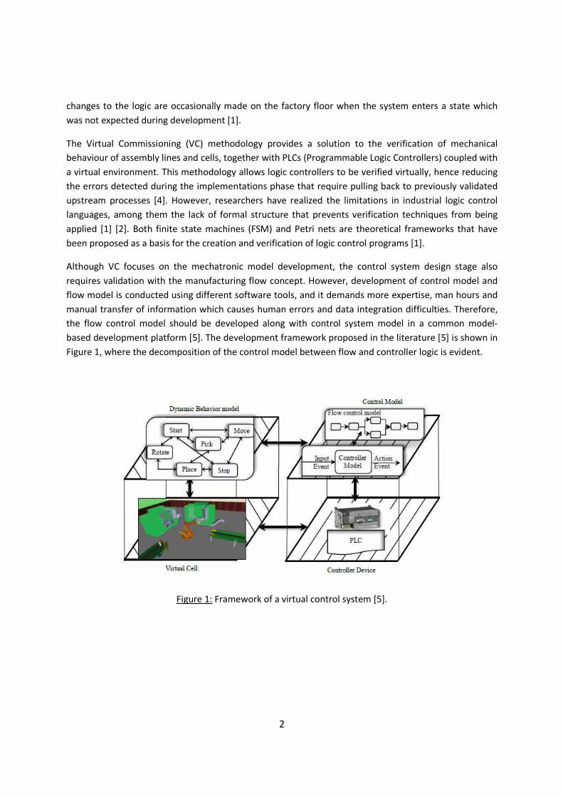
based development platform [5]. The development framework proposed in the literature [5] is shown in
Figure 1, where the decomposition of the control model between flow and controller logic is evident.
Figure 1: Framework of a virtual control system [5].
3
This development stage may also generate long debugging loops between these two tasks, passing the
system design back and forth between both developers until all limitations have been addressed and the
approved solution can be reached and forwarded downstream. Even excluding the validation procedure,
control engineers are in reality involved just in the final stages of the project, where they are required to
develop control strategies to accomplish the specifications previously defined by mechanical/process
engineers, and to program all the mechatronic systems. In fact the real complex control logics will be
designed in detail by control engineers much later in the project, during the last stages of the
manufacturing system development, or even during final implementation and commissioning [6].
These two steps, the validation of the control system and the code generation for the logical controllers
greatly affects development time [7]. This increases the working capital needs of the project and causes
late delivery of the project, and consequent loss of sales opportunities.
Aim
The purpose of this thesis is to implement a concurrent engineering method for control system
development, as part of manufacturing system design. The implementation consists of a parallel
simulation of a flow simulation and a machine control system, in two different computers, to run
together in parallel and real-time. In this way, two development engineers can sit at different machines,
developing a specific level of the manufacturing system, but allowing immediate validation of the
changes made to each system. The data connection between the two computers is to be accomplished
using the OPC technology, an established standard in Networked Control Systems.
The present work is also an implementation of a formal logical method in the creation of control
systems. Simulink, which is the block simulation environment of Matlab, shall be used to model a
control system using Finite State Machines (FSM). The same software also has a PLC coding feature,
which allows automatic PLC code generation from the control system FSM. Although this report doesn’t
cover PLC coding, it’s the main reason for the interest in this implementation.
The intended result can be described as a coupled hybrid system, consisting of two simulation
environments, with two different roles and modelling approach. These two environments work together
as a distributed/parallel simulation.
Task
The main task of this thesis is to establish two simulation models, corresponding to two different levels
of a manufacturing system, each in a different computer. One computer shall run the simulation of the
factory flow as a classical Discrete-Event System (DES), while the other computer shall run the control
systems of the factory’s operations as Finite-State Machines (FSM), a special case of a DES suitable for
logic control. The communication of the two systems shall be accomplished using the OPC technology, a
standard in industrial control systems with previous successful application in real-time industrial
4
communication. This standard uses DCOM technology, and DCOM configuration in the computers is also
an important task in this project, since the communication architecture is intended to be as simple and
direct as possible.
Scope
The purpose of the thesis is to establish a functional single platform of real-time development between
the material flow and the control system. This includes:
♦ Implementation of a communication solution between two instances of a simulation software in
different computers;
♦ Development of a simple example of a manufacturing system with separated control logic;
♦ Troubleshooting of the communication limitations of running the control logic in a separate
system.
Although there is development of a manufacturing system, the scope does not include the actual
development of a manufacturing solution for any real issue, so the system used in the simulation is a
very simple one. The interest of using Finite State Machines in Matlab is related to potential automatic
PLC code generation, which is a subsequent step, out of this report’s scope.
5
Chapter 2
Manufacturing System Development
2.1. Overview
A manufacturing system is essentially a group of manufacturing resources combined to execute a group
of processes, in order to create a product demanded by a customer [8]. During manufacturing system
design, there are some specific activities that are performed by development engineers. These activities
focus generally on typical issues, such as [8]:
♦ The product to be manufactured by the system;
♦ Manufacturing technologies, processes and resources, and their ability to contribute to the
desired product features;
♦ Manufacturing system concepts about the processes, layout, batching, resources, process
control or inventory management.
Many of the specific activities for manufacturing system design are supported by methods developed
and used within the area of operations management. The design of the system’s output (products and
services) follows general problem-solving methods. On the other hand, the design of processes is
executed by modelling through application of a set of special methods for network design, design of
layout and flow, process technology design and job design. Nevertheless, process design is often
executed in parallel with product design [8].
Process technology design deals with the choice of the resources that are going to support execution of
the chosen processes. Such resources may include manufacturing automation technologies, information
technologies and artificial intelligence technologies [8].
2.2. Concurrent Engineering
Overview
Products and manufacturing systems are developed in an organization consisting of specialized
professionals that are responsible for executing one task out of a variety of the development tasks.
6
These professionals are often distributed through the different organizational entities. A product and its
corresponding manufacturing system should be developed both in the product features and the
manufacturing system specific features in a concurrent way. This increases productivity and quality of
the development process. Such work principle, called concurrent engineering (CE), is characterized by an
intensive information exchange between the different development tasks [8].
Traditionally, decisions on these issues were taken in sequence. First, a product design was selected
from a set of feasible designs, according primarily to customer requirements, and technical constraints.
The chosen product design was then used by the production planning team that developed an
appropriate manufacturing plan. Such plans were guided primarily by operational constraints, like cost,
capacity, load balancing, etc. Finally, the product design and the production plan decisions became
constraints for the logistics function that determined the supply sources [9].
This sequential approach is known to generate solutions that suffer from two major deficiencies. First, it
is slow because it assumes an activity must be concluded before the downstream activity can start,
overlooking parallel processing opportunities, and generating time waste on redundant activities.
Second, it leads to sub-optimal solutions, because each stage can only reach a locally optimal solution,
based on previously defined constraints [9]. Often designers do not anticipate the manufacturing
implications of their decisions, resulting in impractical designs which are difficult to cope with by the
following development activities [3]. Therefore, each development engineer tends to work enclosed in
its own field of expertise, with little or no coordination with other disciplines, and to make choices based
on local criteria to produce a globally sub-optimal design. Changes are usually needed and this process
inevitably leads to rework, and increased development cost and time-to-market. The consequences of
inefficient communication among the designers and with other departments are lengthy development
cycles, costly design reworking and ultimately, products that fail in the marketplace [10] [11].
Concurrent Engineering (CE) is a paradigm aimed at eliminating such flaws. CE principles state that
product and process decisions are made in parallel as much as possible and that production
development concerns are incorporated into the product design stage [9]. CE defends a rapid,
simultaneous approach, where all stages of concept development including design, manufacturing, and
support are carried out in parallel. This approach requires developers to consider all elements of the
product life cycle from conception to disposal, including quality, cost, scheduling and user requirements
[10]. There are many examples in literature of advantages in the application of CE to product
development. It reduces development cost by reducing the need for re-design and rework, thus
reducing development time and the amount of rejected development concepts. Furthermore, it
increases the chances for smoother production, which contributes to minimise cost and improve quality,
productivity and service life [9] [11] [12].
One of the basic components of concurrent engineering is the integration of all aspects of the product's
life cycle from the beginning of the development project, as early as possible. This demands flexibility
and integration of all manufacturing concerns during design and planning. Issues related to
manufacturing, assembly, maintenance, and recycling of a product are considered conjointly with design
functions. By looking at these later phases of the life cycle during the design process, it is possible to
7
reveal and tackle problems that might have been detected only at a later time, if a sequential approach
was chosen instead. This concept requires several new approaches to achieve concurrency in complex
multi-disciplinary decisions, based on the large amount of information and possible interactions, and
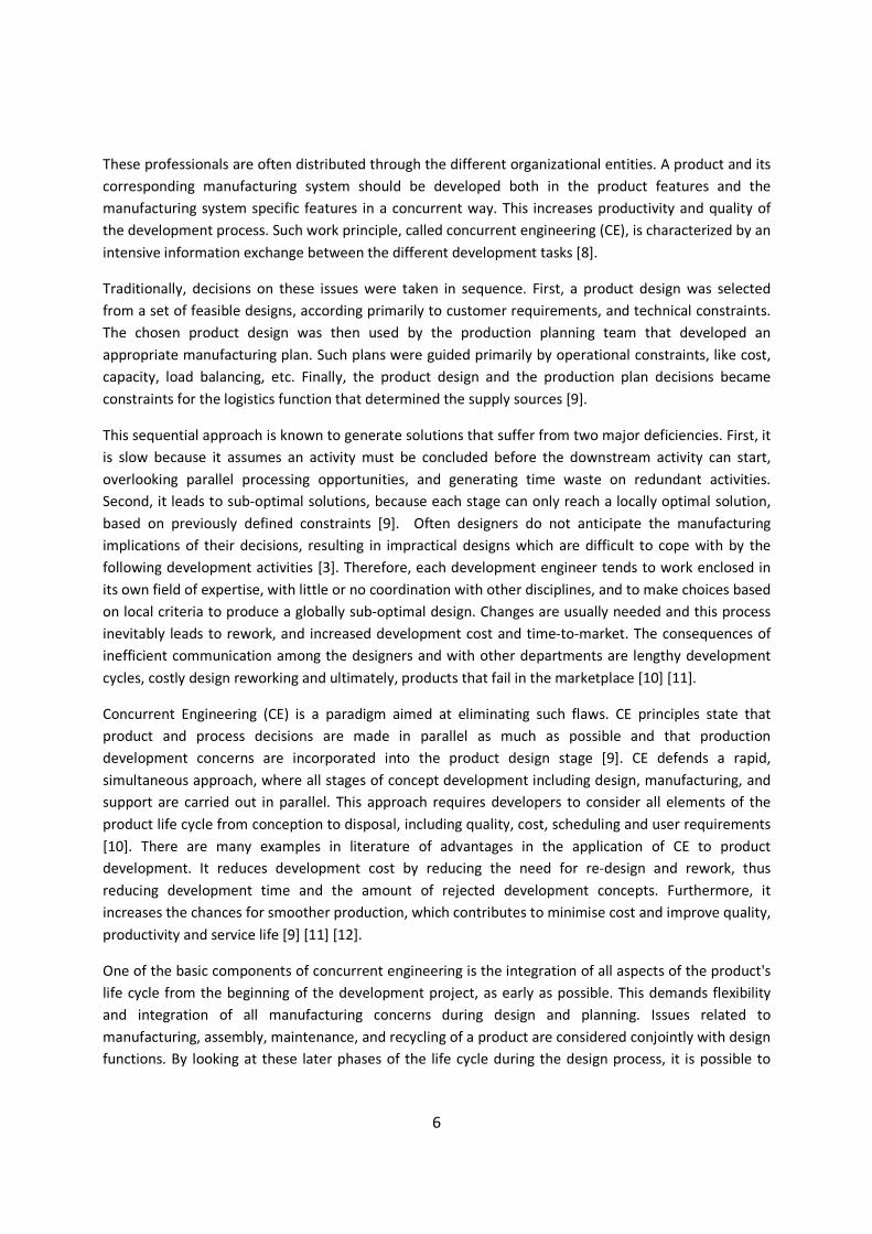
engagement of cross-functional teams. In order to achieve this, knowledge availability is crucial. Typical
decrease in time by applying concurrent engineering compared to sequential engineering is shown in
Figure 2 [10] [12] [13].
Figure 2: Comparison of time savings in the application of concurrent engineering (CE)
and sequential engineering [12].
Applications
Concurrency can be based on the forward effects, backward effects, or combined forward and backward
effects of the processes. In forward effect planning, the dependence of each process on its previous
processes is only taken into consideration for scheduling the activities. It is implicitly assumed that each
stage influences only the following ones. Backward effect planning considers that each stage can
influence its predecessors. For example, a strictly sequential approach where process planning is carried
out after product design usually influences back design results, meaning that considerations specific to
process planning may cause designs to be altered. Production capabilities also have a similar effect on
design and process planning. Overlooking this effect is reported to be the major source of frequent
rework in sequential manufacturing systems planning, so the processes with high backward effect
should be started as early as possible, so to enhance the degree of concurrency of the activities and
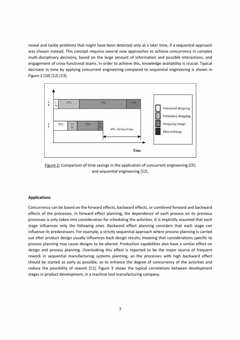
reduce the possibility of rework [11]. Figure 3 shows the typical correlations between development
stages in product development, in a machine tool manufacturing company.
8
Figure 3: Typical CE network in a machine tool manufacturing company [11].
Three major elements of CE implementation are early involvement of participants, team approach and
simultaneous work on different phases of product development [14] [15]:
♦ Early involvement of participants: Early involvement of different functional groups is essential
for cycle time reduction and improvements in product innovation capabilities. This cross-
functional involvement should begin as early as the concept stage, since the most common
cause of delay is related to wrong or missing information. Design characteristics such as
manufacturability, complexity, and design for quality can also be improved through greater
cross-functional involvement. Through a wide functional scope in the acquisition and
interpretation of data, the development team can decrease the ambiguity of customer
information, leading to more robust design.
♦ Product development teams: Cross-functional teams with highly effective communication and
learning capabilities are an important part of CE implementation. Teamwork is understood as a
process of gathering around the common interest of the project, the interdependencies, shared
risks and potential for synergies. This approach allows constant mutual adjustment to
information provided by the rest of the team.
♦ Concurrent work-flow: This element consists of stimulation of parallel activities. With early
release of information, engineers can begin working on different phases of the problem, while
final designs are evolving. While not reducing the duration of each activity, it does decrease the
overall development time. Rework is also avoided due to early detection of design faults.
9
Although many studies show that CE can successfully solve the typical problems of traditional product
development, it is also reported that success depends on the context in which CE is applied. CE may
involve increased cost in comparison with the traditional sequential development, making it more
suitable when reducing development time is a higher priority than reducing cost. In this case, partial
overlapping may also reduce sequential development time, although to a lesser extent, but with a
smaller increase in development cost. Also, the necessary communication amongst the developers may
not be easy to achieve for complex projects, and parallel development may actually slow the project
down [9] [15].
Implementation
From the implementation point of view, the Concurrent Engineering paradigm can be viewed as an
integration of specialized software tools. An efficient integration of CAD, CAE and CAM activities and
inclusion of cross-functional constraints is essential to support the CE paradigm in product development.
Using virtual development environments, designers can estimate several alternative possibilities [10]
[12].
Virtual Engineering (VE) technologies open many possibilities in product and process development by
allowing the developer to model, simulate and optimize the design. However, individually none of the
VE tools is sufficient to satisfy all the design requirements and goals on its own. Therefore, integration of
VE technologies is imperative, particularly when considering the flexibility requirements of industries
like automotive and aerospace. In these cases, several thousand parts for different models and
configurations make it impossible to respond to customer requirements by relying on expensive and
time consuming physical prototypes [12].
Very often, large manufacturing businesses are split-up but coordinated over several continents, usually
to take advantage of low-cost, high quality manufacturing resources in different countries. As a result,
designers need to make a reasonable choice for their products from these manufacturers, or to dispatch
sub-tasks among them according to their respective manufacturing capability and cost. Such an
implementation is possible by using the concept of a multi-agent system, where agents are used to
encapsulate engineering services that can be delivered via the Internet, to cooperate and collaborate
over the Web towards overall system goals [11] [13].
2.3. Virtual Commissioning
The productivity of modern manufacturing systems is assured by highly automated, fast operating
systems. As markets become more demanding in customized solutions, products become more complex
and so do their corresponding assembly processes. This is clear in the increasing complexity of control
system development. These systems include the activation, coordination and monitoring of most of the
10
machine functionality, and represent the core of an automation system. Testing and validating a
designed control program is rarely possible without the controlled mechanical elements. Even if these
elements are available, the processes under testing are usually too fast for developers to interact with
[7].
Virtual Commissioning (VC) as a concept is understood as virtual implementation and validation of
industrial automation systems using virtual tools prior to the implementation of the real system [5]. It
allows the coupling of simulation models to real-world entities and enabling the analyst to pre-
commission and test a system’s behaviour, before it is built in reality. A VC project involves three distinct
but interconnected subsystems [4] [16]:
♦ The mechanical design, including actuators, sensors, and behavioural description of a system
related functional model;
♦ The machine control, including its input and output signals;
♦ The signal connections between sensors/actuators and the control.
This methodology attempts to provide faster and more reliable control logic implementation. As the
product cycle times has shortened over the last few years, so did the lead time for new manufacturing
systems. Consequently, control logic implementation processes have become more frequent. Although
there is a trend of product, equipment, and process standardization, it is not by itself capable of assuring
that the designed assembly and production systems will be fully operational after their physical
deployment. The complexity and diversity of the different line components, in terms of control systems
and communication channels, requires a great amount of time for onsite setup, testing, and validation
of the assembly equipment. This causes production system downtime and the respective opportunity
costs that follow it [4] [16].
Digital simulation of the assembly process has emerged recently as a means of partially validating
manufacturing systems before their installation. These simulation systems are based on the digital
factory/manufacturing concept, according to which production data management systems and
simulation technologies are jointly used for manufacturing system optimization before starting the
production, offering supporting to the implementation phases [4]. VC goes a step further by including
more validation capabilities by simulating the mechatronic behaviour of the resources. The VC
methodology allows the verification of the mechanical behaviour of assembly lines and cells, in
conjunction with PLCs (Programmable Logical Controllers) in loop with a virtual environment [1]. Such
virtual environments are capable of simulating kinematics, geometric, electric, and control-technical
aspects, providing a full-scale mapping of the real system and the control system under development
[4].
Currently, there are two approaches to building a VC project. Under the Software in the Loop (SIL)
method, the control programs for the resource controllers (PLC or other) are downloaded to virtual
controllers and TCP/IP connection is established between the mechatronic object and the virtual
controllers. It is obvious that the main advantage of the SIL approach is that no hardware is required
during the design and validation of control software, as a standard PC is suitable for implementation.
11
The second method, known as hardware in the loop (HIL), involves the simulation of production
peripheral equipment in real time, connected to the real control hardware. Under this setup,
commissioning and testing of complex control and automation scenarios, under laboratory conditions,
can be carried out for different plant levels [4].
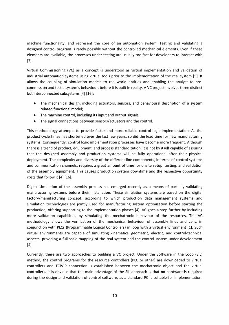
The validation of a VC project of a control system requires the interaction of two different
environments. The first environment is the 3D simulation model, which represents the cell layout, with
the resources geometry and the kinematic constraints that model the resource behaviour. The second
environment is used for the emulation of the control signals and the signal exchange networks, which
are used within the cell, either by robots or any other devices such as safety equipment, human-
machine interfaces, and so forth [4] [5]. Variations may include more than one system in the simulation
environment (separation between visual and logical simulation), as depicted in Figure 4 [7].
Figure 4: Virtual Commissioning through the coupling of a control system
with a running simulation and a 3D-visualization [7].
2.4. Networked Control Systems
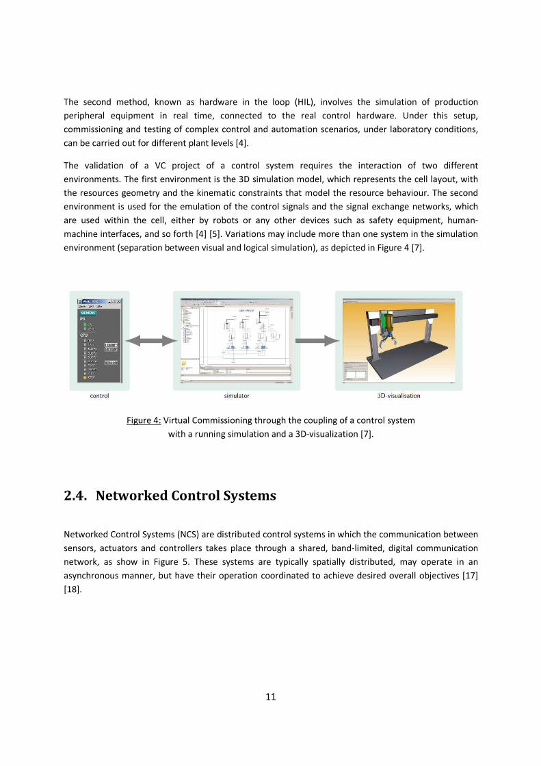
Networked Control Systems (NCS) are distributed control systems in which the communication between
sensors, actuators and controllers takes place through a shared, band-limited, digital communication
network, as show in Figure 5. These systems are typically spatially distributed, may operate in an
asynchronous manner, but have their operation coordinated to achieve desired overall objectives [17]
[18].
12
Figure 5: General architecture of a Networked Control System.
Initially, control of manufacturing and process plants was done mechanically - either manually or
through the use of hydraulic controllers. With the development and increased popularity of discrete
electronics, the mechanical control systems were replaced by electronic control loops employing
transducers, relays and hard-wired control circuits [19]. These hardwired control systems were designed
to bring all the information from the sensors to a central location where the all decisions were made on
how to control the system. The control policies then were implemented via the actuators, which could
be valves, motors, etc. These systems were large and space consuming, often requiring many kilometres
of wiring, both to the field and to interconnect the control circuitry [18].
With the invention of integrated circuitry and microprocessors, multiple analogue control loops could be
replaced by a single digital controller. The movement toward digital systems brought new
communications protocols to the field as well as between controllers, referred to as fieldbus protocols.
More recently, digital control systems started to incorporate networking at all levels of the industrial
control, as well as the inter-networking of business and industrial equipment using Ethernet standards.
This has resulted in a networking environment that appears similar to conventional networks at the
physical level, but which has significantly different requirements [19].
2.4.1. OPC Servers
Since the early nineties, the use of software-based automation has rapidly increased, particularly with
the introduction of Microsoft Windows operated computers for visualization and control purposes. As a
consequence, it became important to develop standardized automation software to cope with the issue
13
data availability across devices, where several different bus systems, protocols and interfaces are used
[20]. An example of this issue was faced by the software vendors of HMI (Human-Machine Interface)
and SCADA (Supervisory Control and Data Acquisition) systems [20]. SCADA software systems are used
in the automation industry for applications such as systems for industrial measurement, monitoring and
control. Most current SCADA systems were designed by a single company for a specific system, because
there were few generally accepted interfaces. Therefore, it was not possible to include components
from a different vendor into the system, as the data structures were proprietary and not able to
communicate outside the implemented system [21].
A similar problem happened in domestic computer systems, in the connection between software
applications and printers. In the 1980’s, when computers were running command line based DOS, every
application vendor needed to write its own printer drivers for all supported printers. Microsoft Windows
solved this problem by incorporating printer support into the operating system. So, one printer driver
served all applications, and this single printer driver was provided by the printer manufacturer instead of
the different application developers [20].
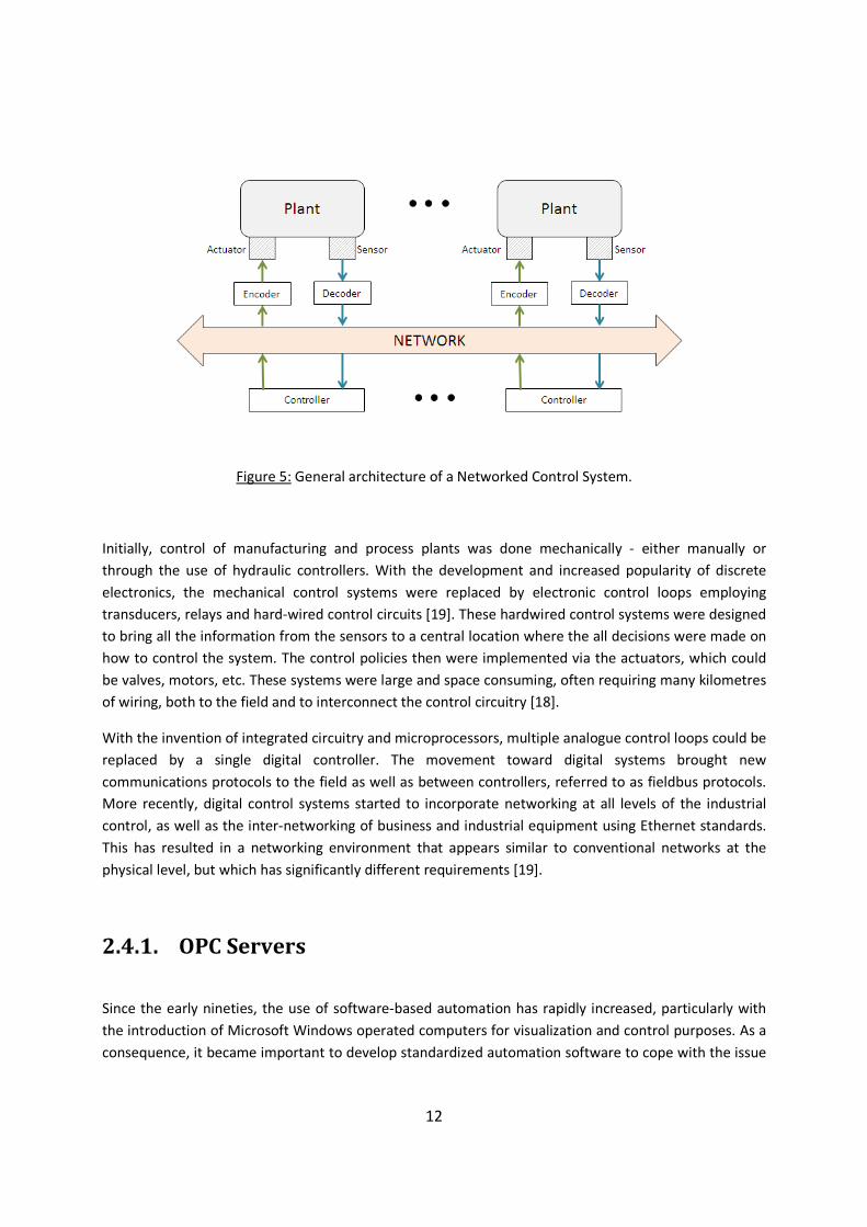
Figure 6 gives an example of conventional communication architecture between different software
application and three different process control devices used in the manufacturing Industry. To be able to
communicate with the devices in the system, each software application in the system needs a driver for
each device, rendering the system expensive and making data transfer more complex [21].
Figure 6: Conventional communication architecture [21].
In order to address this lack of flexibility, a task force was established in 1995 to define a common
standard for access to automation data, in a Microsoft Windows based environment. This lead to the
creation of the first OPC specification the following year, named OPC Data Access or just OPC DA. [20].
Originally, OPC stood for OLE for Process Control, while more recently it has changed into Openness,
Productivity and Collaboration [23] [24].
14
OPC is an open and flexible communication standard in the process supervision field that allows
software applications or process modules to interact and share data. This is accomplished by defining a
standard set of objects, interfaces and methods that are used in process control and automation
applications to enable interoperability between them [22].
The motivation behind OPC is to develop a standard mechanism for communication to several data
sources, either factory floor devices or control room databases and interfaces. It means to standardize
data access to data in industrial applications, by allowing several different clients to access the data
managed by an OPC server, through a MS Windows network [21]. In short, OPC technology makes it
easier for software and hardware from different sources to integrate and allows remote real-time
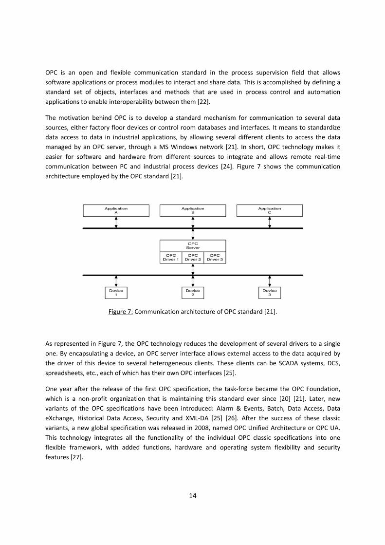
communication between PC and industrial process devices [24]. Figure 7 shows the communication
architecture employed by the OPC standard [21].
Figure 7: Communication architecture of OPC standard [21].
As represented in Figure 7, the OPC technology reduces the development of several drivers to a single
one. By encapsulating a device, an OPC server interface allows external access to the data acquired by
the driver of this device to several heterogeneous clients. These clients can be SCADA systems, DCS,
spreadsheets, etc., each of which has their own OPC interfaces [25].
One year after the release of the first OPC specification, the task-force became the OPC Foundation,
which is a non-profit organization that is maintaining this standard ever since [20] [21]. Later, new
variants of the OPC specifications have been introduced: Alarm & Events, Batch, Data Access, Data
eXchange, Historical Data Access, Security and XML-DA [25] [26]. After the success of these classic
variants, a new global specification was released in 2008, named OPC Unified Architecture or OPC UA.
This technology integrates all the functionality of the individual OPC classic specifications into one
flexible framework, with added functions, hardware and operating system flexibility and security
features [27].
15
The OPC standard is based on OLE/COM technology, which is the most important client/distributor
technology of Microsoft. OLE and COM objects of Microsoft are available in Microsoft’s Visual Basic,
Visual C++ and Borland’s Delphi software packages [21]. The OLE protocol was developed to cover the
disadvantages of its preceding DDE protocol. DDE represented the first solution for data exchange
between Microsoft Windows applications. However, it bears the disadvantage of low bandwidth, which
limits its use in real-time systems [21].
Microsoft COM (Component Object Model) technology enables software components to communicate
in the MS Windows family of operating systems. COM is dedicated to communication openness and
speed, and is used by developers to create re-usable software components, link components together to
build applications, and take advantage of Windows services. The family of COM technologies includes
COM+, Distributed COM (DCOM) and ActiveX® Controls [28]. It defines interaction mechanisms
between objects, including application objects and data objects. The basic communication method used
in the COM platform is based on synchronous input/output processing. This means that the calling
object waits for a response from the method called, in a mechanism that corresponds to a client/server
model [21].
Data exchange between OPC client applications and OPC servers can be done in three different ways:
synchronous, asynchronous and subscription. Synchronous exchange is simple when there is a low
amount of data. Asynchronous allows direct communication with the devices, and allows efficient
communication of larger amounts of data. By using the subscription way the server notifies the client
application when the data changes [24]. The OPC Toolbox in Matlab allows Matlab and Simulink to
interact with OPC servers. It is possible to write, read and log data from devices that support the OPC
Data Access standard, in synchronous or asynchronous mode [29].
Researchers have used OPC servers to connect Matlab/Simulink and a SCADA system, to provide higher-
level solutions, with increased economic relevance and multi-purpose objectives, making full use of real-
time communication capabilities [25] [29] [30]. Other studies show OPC application in fault detection
and diagnosis in real-time [22], distributed OPC over internet [21] and UDP communication using Matlab
[31]. Also reported is the usage of OPC servers in other embedded systems, making full use of its
capability of connection between HMI systems, XML configuration files and legacy calibration systems
[1] [22].
16
Chapter 3
Parallel and Distributed Simulation
3.1. Overview
Parallel and distributed simulation is about using multiple interconnected computers in a single
simulation. It combines the technologies for simulation and execution on parallel or distributed
computers [32] [33]. The main benefits of this approach are [33]:
♦ Reduced execution time, by subdividing a large computation into many sub-computations;
♦ Geographical distribution, which allows collaboration of multiple users in different locations;
♦ Integrated simulation, which allows simulations to run on different machines from different
manufacturers.
♦ Fault tolerance, by having redundant processors to continue the work of a failed machine.
Parallel and distributed computing platforms differ in the hardware used, as it’s summarized in Table 1
[33].
Table 1: Comparison between parallel and distributed computer platforms [33].
Parallel Computers Distributed Computers
Physical extent Machine room Single building or global
Processors Homogeneous Often heterogeneous
Communication network Customized switch Commercial LAN or WAN
Communication latency < 100 µs Hundreds of µs to seconds
17
Technology
Parallel computation requires synchronization across the multiple processors involved. The simulation is
divided both spatially or temporally, and all processors together simulate collectively an integrated set
of application models [32]. To be successful, the results produced by a parallel simulation run must
match those produced by an equivalent single simulation run. To achieve this, its main focus is on
accurate synchronization of all the simulations running on multiple inter-connected processors. Proper
synchronization preserves the right execution orderings and dependencies during computation across
processors [32]. One of the challenges in this synchronization is in minimizing the execution overheads
(memory, computation and communication) that occur during parallel execution. It is important to keep
the overhead within acceptable levels, so that the parallel execution becomes at least as effective as the
classical single-processor simulation [32].
Parallel and distributed simulations can be classified as spatial parallel or time parallel. In spatial parallel
simulation, the application is broken down across a spatial dimension intrinsic to the application’s
models, which could be positions in a grid or computer addresses. Time parallel simulations divide the
simulation in time intervals along the simulation time axis [32] [34]. Spatial decomposition is by far the
most commonly used parallel simulation scheme. In this scheme, application models are divided into
logical processes (LP). Each LP contains its own individual state variables, and interactions among LPs are
carried out through exchange of time-stamped events. The simulation progresses via execution of these
events in temporal order, which is either maintained at every instant during simulation, or is achieved in
an asymptotic manner (i.e., the system guarantees eventual convergence to overall temporal order)
[32].
Synchronization of parallel/distributed simulation is described using the following concepts:
♦ Notion of Time: In simulations there are generally three distinct notions of time. The first is the
physical time, which is the absolute time in the physical system that is being modelled
(e.g.,10:00:00am on the 3rd of January 1990). The second is the simulation time, which is a
relative representation of the physical time (e.g., number of seconds since 10:00:00am of the 3rd
of January 1990, represented in floating point values). Finally, the wallclock time is the elapsed
real time during execution of the simulation, as measured by a hardware clock (e.g., number of
milliseconds of computer time during execution). For each, the notions of time axis and time
instant can be defined [32] [33].
♦ Execution Pacing: There is usually a one-to-one relationship from physical time to simulation
time. However, there may or may not be an exact relationship between simulation time and
wall-clock time. In an as-fast-as-possible execution mode, the simulation time is advanced as
fast as the processor speed is capable of, unrelated to wall-clock time. In real-time execution
mode, one unit of simulation time corresponds exactly to one unit of wall-clock time [32].
♦ Events and Event Orderings: Simulation events indicate updates to simulation system states at
specific time instants. Therefore, each event has a specific timestamp. Event sending and
delivery between processors needs to be carefully coordinated at runtime. In general, two
18
different delivery ordering systems can be defined, timestamp-order and receive-order. In
timestamp-ordered delivery (TSO), events are guaranteed to be delivered in the same order they
were sent, according to the information in their timestamps. In receive-ordered delivery (RO),
events from the sending processor are delivered as soon as they arrive, without regarding their
timestamp. Typically RO delivery incurs lower delivery delay/latency between sending and
delivery. On the other hand, TSO events are subject to higher latency, since they are checked
and buffered during runtime to make ensure the right timestamp order. However, RO cannot
always preserve “before and after” relationships, while TSO preserves such relationships, even
across multiple processors, which grants the repeatability of the simulation unlike RO delivery
[32].
The synchronization issue in parallel simulation is related to the need to assure that events are
processed in their timestamp order. There are generally four approaches commonly used to overcome
this problem: conservative, optimistic, relaxed, and combined synchronization [32] [33] [35]:
♦ Conservative: This approach always ensures that a logical process does not execute an event
until it can guarantee that no event with a smaller timestamp will later be received by that LP.
However, this involves determination of a property named lookahead, which is the forward time
interval to which the LP can foresee future interactions without global information. Events
beyond the lookahead window are blocked while waiting.
♦ Optimistic: This approach allows processing of events beyond the lookahead interval. In complex
parallel simulation systems, there is an increased risk of delay in communication between
processors. By allowing the computation to progress at all times, this approach attempts to
address that delay. Although effective in this sense, it may require the simulation developer to
include algorithms that enable rolling back to a previous state, in case the timestamp arrival
order is broken.
♦ Relaxed synchronization: This approach removes the timestamp order constraint, allowing two
events to be processed if their timestamps are close enough. This allows a simplified
synchronization, but it requires setting the extent to which timestamps can be delayed without
compromising the simulation’s repeatability..
♦ Combined synchronization: This approach combines elements of the previous three approaches,
taking advantage of the distributed and partially independent nature of parallel simulation
systems.
Applications
Parallel and distributed simulation finds relevance in many fields, including civilian applications such as
telecommunication networks, physical system simulations and entertainment, and non-civilian
applications such as battlefield simulations and emergency event training exercises [32] [33].
19
Parallel simulation is a promising methods in networked control system (NCS) simulation, to make
different tools work together to simulate different parts of the overall system concurrently. The co-
simulation strategy can also be seen as a framework to support future co-design of both the control part
and the communication network part. Compared with individual simulators, co-simulation method has
the following advantages [36]:
♦ The overall behaviour of the NCS application becomes observable, which is not possible when
simulating either the control or the communication system separately. For example, one can
observe the effects of network topology, medium access, routing protocols, and traffic pattern
on overall control system performance.
♦ It is possible to analyse large complex systems with multiple control loops, which cannot be
done mathematically.
There is literature on the usage of distributed discrete event systems (referred to as Parallel DES) for
simulation of supply chains. In such case, distributed processing of the models of the constituent units
may potentially reduce the communication overhead and improve execution time significantly,
improving the feasibility of the simulation of such systems [35].
In manufacturing applications, there is research on the development of a distributed integration
platform that supports the whole life cycle of agile modular machine systems. This platform includes the
design, simulation, programming, analysis, machine operation and re-configuration. This environment
supports distributed management and storage of information in a system-wide library, information
management and storage that is machine-oriented, instead of application oriented, and information
storage structured as reusable components to enable reuse of information that is produced throughout
the life cycle of machines [3].
3.2. Discrete Event Systems
The concept of Discrete Event System (DES) was introduced in the early 1980’s to identify systems
whose behaviour is governed by discrete events occurring asynchronously over time. Such discrete
events generate state transitions, which remain unaffected between event occurrences [37].
Discrete event systems has been used as a methodological tool in simulation. Indeed, given a set of
inputs which are expected to influence a set of outputs, DES appears as an effective tool to highlight the
actual relationships when the model shows high variance. The ability of DES to support ‘‘what-if’’
analyses and to provide quantitative results is well documented, so it’s successfully used in business
processes re-engineering projects [38]. There are several examples of this behaviour in technological
applications, such as computer and communication networks, automated manufacturing systems, air
traffic control systems, advanced monitoring and control systems in automobiles and buildings,
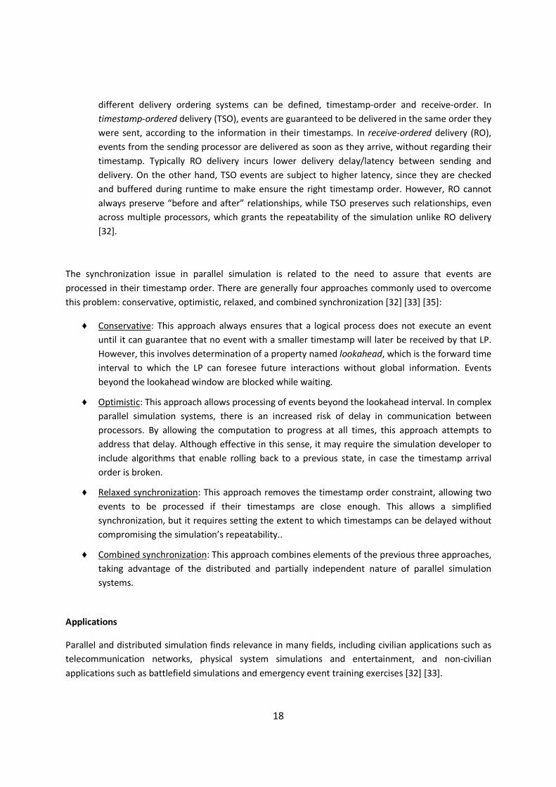
intelligent transportation systems, distributed software systems, etc. [37]. Figure 8 shows a simple
example of a DES, modelled in two different simulation software environments.
20
a)
b)
Figure 8: Graphical DES models of a simple transfer line.
a) Using ExtendSim; b) Using Matlab/Simulink
A DES is a discrete-state, event-driven system, i.e. its state evolution depends entirely on the occurrence
of asynchronous discrete-events over time. These systems are often operated by human-made rules,
which initiate or terminate activities according to controlled events, such as a keyboard input, a switch
or a message packet. Additionally, random events can occur, such as a spontaneous failure, which may
be observable or not [37]. Many technological systems are in fact discrete-event systems. Even when it’s
not the case, it is necessary in many applications to consider a discrete-state approach for simplification
of complex systems. Some examples of DES include [39]:
♦ The state of a machine can be { ON, OFF } or { BUSY, IDLE, DOWN }
♦ A computer running can be viewed as being { WAITING FOR INPUT, RUNNING, DOWN }. Also,
the RUNNING state can be broken down into several individual states.
♦ Any type of inventory consisting of discrete entities (e.g. products, money, people) has a natural
state space of non-negative integers { 0, 1, 2, … }
♦ Most games have a discrete state space. For example, in chess every possible board
configuration is a state. Although the state space is huge, it is discrete.
As mentioned, in DES the events causing state transitions are asynchronous, i.e. the system’s states
don’t change continuously and regularly over time. Therefore, it is neither natural nor efficient to use
time as a synchronizing element driving the system’s dynamics. For that reason, these systems are often
referred to as event-driven, as opposed to time-driven systems, where state variables evolve
continuously according to time. Uncertainties are inherent in the technological applications where DES
are found. Therefore, the mathematical models used for DES and all associated methods for analysis and
control must consider this element of uncertainty, sometimes by explicitly modelling stochastic
behaviour [37].
21
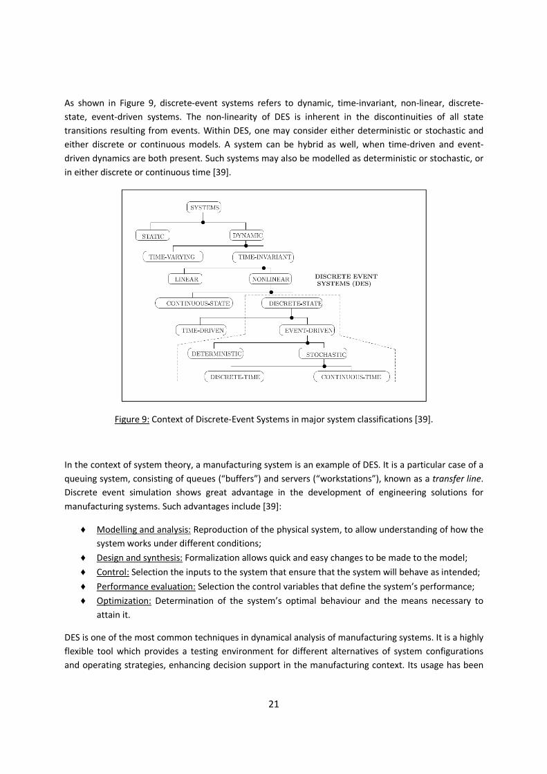
As shown in Figure 9, discrete-event systems refers to dynamic, time-invariant, non-linear, discrete-
state, event-driven systems. The non-linearity of DES is inherent in the discontinuities of all state
transitions resulting from events. Within DES, one may consider either deterministic or stochastic and
either discrete or continuous models. A system can be hybrid as well, when time-driven and event-
driven dynamics are both present. Such systems may also be modelled as deterministic or stochastic, or
in either discrete or continuous time [39].
Figure 9: Context of Discrete-Event Systems in major system classifications [39].
In the context of system theory, a manufacturing system is an example of DES. It is a particular case of a
queuing system, consisting of queues (“buffers”) and servers (“workstations”), known as a transfer line.
Discrete event simulation shows great advantage in the development of engineering solutions for
manufacturing systems. Such advantages include [39]:
♦ Modelling and analysis: Reproduction of the physical system, to allow understanding of how the
system works under different conditions;
♦ Design and synthesis: Formalization allows quick and easy changes to be made to the model;
♦ Control: Selection the inputs to the system that ensure that the system will behave as intended;
♦ Performance evaluation: Selection the control variables that define the system’s performance;
♦ Optimization: Determination of the system’s optimal behaviour and the means necessary to
attain it.
DES is one of the most common techniques in dynamical analysis of manufacturing systems. It is a highly
flexible tool which provides a testing environment for different alternatives of system configurations
and operating strategies, enhancing decision support in the manufacturing context. Its usage has been
22
favoured by the increase in computer power and memory over the last few years, as it is a demanding
tool in terms of computation. DES applications in manufacturing include manufacturing system design
and manufacturing operations design, which include [40]:
♦ Manufacturing system design:
> General system design/layout planning
> Material handling system design
> Manufacturing cell design
> Flexible manufacturing system design
♦ Manufacturing operations design:
> Manufacturing planning and scheduling policies
> Maintenance operations planning
> Real-time control system design
There is a wide range of successful applications of DES in different areas such as design, planning and
control, strategy making, resource allocation, training, etc., as well as applications in lean manufacturing
tools [41] [42]. Increasing competitiveness and the need to reduce costs and lead times are driving the
increased use of simulation, along with the availability of affordable and intuitive simulation systems
[41].
DES has also been extensively used in modelling and simulation of material and information flow. Apart
from manufacturing, there are known applications of DES to communication systems, supply chains,
marketing, healthcare and military [38] [40] [43]. There are several simulation environments capable of
modelling discrete-event systems. Mathworks’ Matlab, in its Simulink environment [44], and also
ExtendSim (by Imagine That Inc.) [45] and Arena (by Rockwell Automation) [46].
3.3. Finite State Machines
Overview
A Finite State Machine (FSM) is a system that is described as multiple finite states that the system may
assume. The state machine has a set of inputs and outputs, and the ability to maintain its current state
in memory. The system progresses from one state to another depending both on the inputs and the
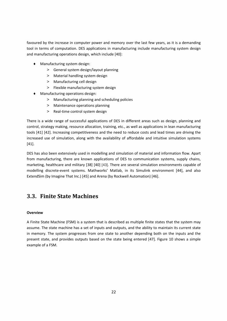
present state, and provides outputs based on the state being entered [47]. Figure 10 shows a simple
example of a FSM.
23
Figure 10: A simple example of a FSM: ventilation control system. The ventilation
is switched on or off according to a temperature input, and outputs a status.
A FSM is a simplified Petri net, which is one the possible modelling formalisms in the context of discrete-
event systems (DES). Like a FSM, Petri nets manipulate events according to previously defined rules, but
the main difference is that an FSM includes explicit conditions under which an event can be enabled.
Although FSMs can always be represented as Petri nets also, not all Petri nets can be described as FSMs.
Still, the choice between both formalisms depends on the particular application considered. Simple Petri
nets can be represented as Petri net graphs, which is an intuitive form of summarizing relevant system
data. [39].
Background
Finite state systems, or finite automata [48], can be modelled as transducers that produce outputs on
their state transitions, upon receiving certain inputs. Mathematically, a FSM can be formulated as a
quintuple M= {I, O, S, δ, λ}, where I, O and S are finite sets of input symbols, output symbols and states.
δ is the state transition function and λ is the output function. So, when a machine is in state s (contained
in S), and receives an input a (contained in I) it moves to the next state specified by δ(s,a) and produces
an output given by λ(s,a) [49].
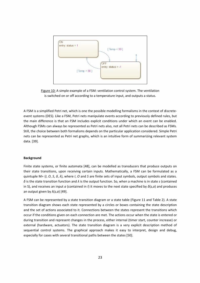
A FSM can be represented by a state transition diagram or a state table (Figure 11 and Table 2). A state
transition diagram shows each state represented by a circles or boxes containing the state description
and the set of actions associated to it. Connections between the states represent the transitions which
occur if the conditions given on each connection are met. The actions occur when the state is entered or
during transition and represent changes in the process, either internal (timer start, counter increase) or
external (hardware, actuators). The state transition diagram is a very explicit description method of
sequential control systems. The graphical approach makes it easy to interpret, design and debug,
especially for cases with several transitional paths between the states [50].
24
Figure 11: Example of a state diagram. Every transition represents the event that
triggers it and the transition output value [49].
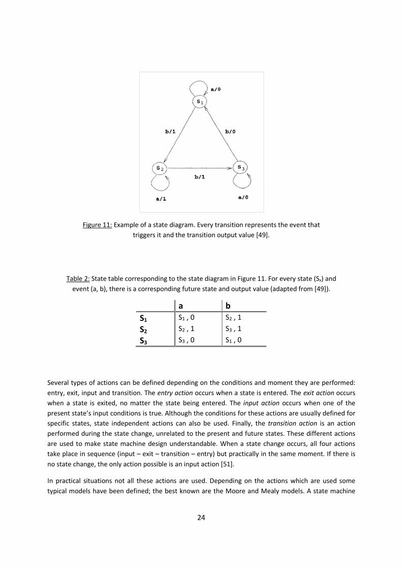
Table 2: State table corresponding to the state diagram in Figure 11. For every state (Sx) and
event (a, b), there is a corresponding future state and output value (adapted from [49]).
Several types of actions can be defined depending on the conditions and moment they are performed:
entry, exit, input and transition. The entry action occurs when a state is entered. The exit action occurs
when a state is exited, no matter the state being entered. The input action occurs when one of the
present state’s input conditions is true. Although the conditions for these actions are usually defined for
specific states, state independent actions can also be used. Finally, the transition action is an action
performed during the state change, unrelated to the present and future states. These different actions
are used to make state machine design understandable. When a state change occurs, all four actions
take place in sequence (input – exit – transition – entry) but practically in the same moment. If there is
no state change, the only action possible is an input action [51].
In practical situations not all these actions are used. Depending on the actions which are used some
typical models have been defined; the best known are the Moore and Mealy models. A state machine
a b
S1 S1 , 0 S2 , 1
S2 S2 , 1 S3 , 1
S3 S3 , 0 S1 , 0
25
that generates only entry actions is called a Moore model while a state machine that generates only
input actions is called a Mealy model [51]. This means that Mealy machines provide an output during
transition, based on the current state and the input, while Moore machines provide inputs based on the
current state alone. The models selected will influence the system’s design, but the choice of a model
depends on the application, execution means, and personal preferences of a designer or programmer
[51].
Applications
Discrete event systems such as FSM have been growing in popularity for control system development,
since control logic is better explained with discrete states than the approach with differential equations.
State transition techniques show the sequential behaviour of the system explicitly, which poses as an
advantage towards classical control logic design methods, such as relay logic which uses combinatorial
methods The state transition concept is also widely used as a method for software code design and
analysis [50]. Alongside FSMs, also Petri nets find application in modelling of control systems [52].
Mathworks’ Matlab is capable of modelling control logic using FSM by using the Simulink environment,
specifically Stateflow charts [53]. A separate toolbox allows automatic generation of IEC 61131-3
Structured Text code from the Simulink modelled control logic, which can then be deployed into a
Programmable Logic Controller (PLC) or a Programmable Automation Controller [54] [55].
Other applications in manufacturing include remote machine tool control, process planning and
scheduling. An FSM can interact with a task list, resource management module, human interface and
executor module, as a solution for the lack of flexibility of planning at machine tool level [47]. It has also
been used for energy requirements simulation and auditing, using a precise definition of different
machine states and their respective power requirements [56] [57] [58].
A FSM can model engineering and biological applications, among which are communication protocol
design, electronics design, automation, neurological systems and many others [59]. Other fields of
application for FSM include genetics [60] [61], language [62] and artificial intelligence [63].
26
Chapter 4
Methodology
This thesis intends to establish a communication platform for two simulation software environments to
communicate in real time. It is proposed to use the current knowledge in parallel and distributed
simulation to propose a solution to a specific problem in the field of manufacturing system
development.
The accomplishment of this objective is made in two separate domains, each with two main goals. The
first domain is communication realization, which addresses the communication configuration and client
application setup. The second domain is platform design, which addresses the model design and the
model distribution. These four stages are explained ahead, and are represented in Figure 12.
4.1. Communication realization
a. Communication configuration
This step concerns the setup of the communication hardware and software to be used in the
common platform (Figure 12, A). The hardware setup consists of two PCs connected to each
other by LAN cables through a network switch. These two computers are configured to work on
the same private network, through TCP/IP protocol, using the appropriate Microsoft Windows
setting. No other networks are present, such as internet or university internal network.
This implementation is conducted using the OPC DA specification to connect two PCs operated
by Microsoft Windows 7. The OPC server software used is the OPC Server for Simulation, by
Matrikon Inc., a Honeywell International subsidiary. For registered users, this software is
available for free as it is mainly destined for test purposes, not business operation [64]. The OPC
technology is based on DCOM, so most of the communication realization consists on the
configuration of the Windows operating system to allow DCOM data exchange. Matrikon
provides tutorial documentation to tackle this issue.
The OPC connectivity between the computers is considered as achieved, as soon as it is possible
to access and browse the other computers’ installed OPC servers and data items.
27
b. Client application setup
This stage is about setting up the communication between the simulation software environment
and the communication server in each computer (Figure 12, B).
The software used for both the flow simulation and the control system was Mathworks’ Matlab,
specifically the Simulink environment. Matlab 7.0 and later versions have an optional plugin for
OPC interface - the OPC Toolbox - which is a function library to replace the MATLAB numerical
calculations environment, which also includes a Simulink block library. It uses the OPC DA
standard to read or write OPC data directly in the MATLAB environment.
The initial intention was to use ExtendSim for the flow simulation, since it’s a specific software
for that purpose, having also been used for DES training in KTH courses. However, the available
version (8.0) was not able to communicate through OPC. This software was able to
communicate through the DDE protocol, so attempts were made to establish a DDE/OPC
communication. DDE is a legacy application communication protocol by Microsoft, where every
object inside an application can be accessed from other application through the use of a link
with a specific syntax. There is an OPC Server for DDE, provided by Matrikon under a trial
license, which was used to attempt the DDE/OPC connection with ExtendSim. However, the DDE
link was not accepted by the server for unknown reasons, even using Microsoft Excel as an
intermediate for the data objects. The idea was abandoned, as it would probably deviate
outside the scope of the thesis to implement it. It was then considered more practical to
develop the DES flow simulation in Matlab/Simulink.
This stage intends to create read and write functions in Simulink environment to test the
effectiveness of the client-server interface, and adjust the reading and writing intervals for
better performance.
4.2. Platform design
a. Model design
At this stage, the simulation is designed in one computer, in a single environment containing the
flow simulation and the control system embedded into it. No OPC communication is configured
at this point, as this stage was meant to develop and troubleshoot the model, especially the
control system, and also to learn about the Simulink environment and Finite-State Machines
design (Figure 12, C).
The scope of this thesis is about the communication platform, and there is no specific real life
manufacturing system development issue to address. Therefore, the flow model and the control
system model will be deliberately simplified for clarity purposes. It is possible that the thesis’
research question may be more fitting to a system comprising a manufacturing cell with robot
28
and conveyor controls. However, the modelled system will consist of a simple transfer line
manufacturing system, with two workstations, routing decisions and queues.
The control system logic shall be simulated for four elements of the flow: the routing device, the
queue level control system in workstation 1 and the state control in each of the two
workstations.
The model is fully built in Matlab’s Simulink environment. It comprises a discrete event
simulation built mainly with the SimEvents block library, and the embedded control logic built
with Stateflow charts.
b. Model distribution
The whole platform design stage corresponds to splitting the simulation model into two
separate models, and linking them to the OPC server to allow reading and writing of common
variables (Figure 12, D). This stage includes:
♦ Creation of isolated simulations for the flow simulation and the control logic;
♦ Definition of the OPC data items;
♦ Introduction of OPC “Read” and “Write” functions into the separate simulations;
♦ Changing the simulation’s models to accommodate communication over an external
server.
In this last stage, it’s very important to consider that the server is an external environment. The
main issue to solve is the synchronization of the two models. The distributed model should
provide the same behaviour and results as the original single model in a single environment.
Model distribution will be accomplished in two steps. First, the previously designed model is
split and executed in the same computer through the OPC server. Only after successful
troubleshooting will the two complementary models be executed in different machines, in order
to isolate the limitations of each step, and address those limitations gradually.
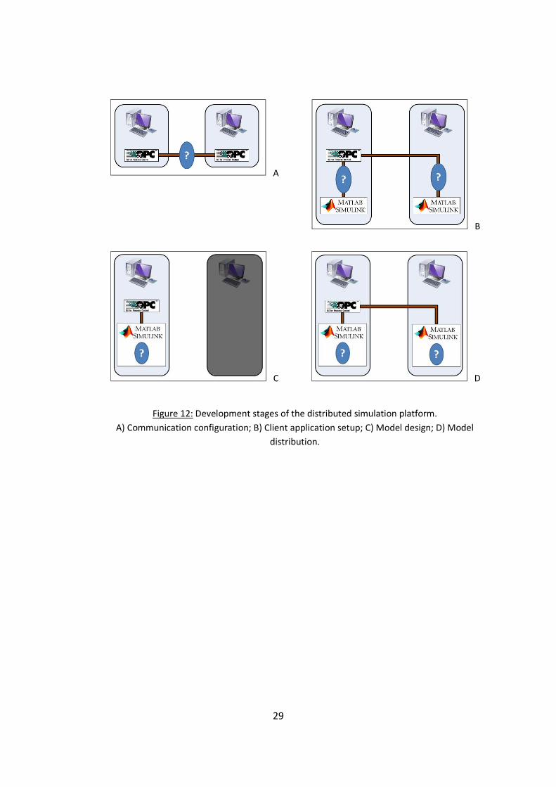
29
A
B
C D
Figure 12: Development stages of the distributed simulation platform.
A) Communication configuration; B) Client application setup; C) Model design; D) Model
distribution.
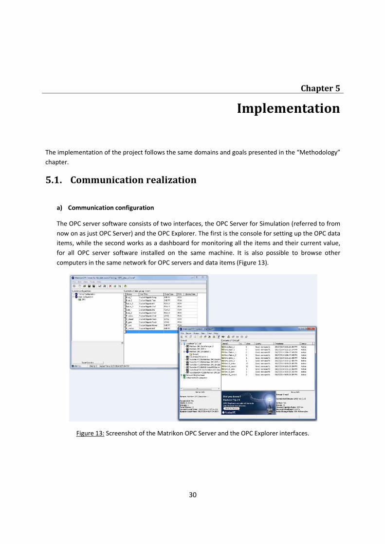
30
Chapter 5
Implementation
The implementation of the project follows the same domains and goals presented in the “Methodology”
chapter.
5.1. Communication realization
a) Communication configuration
The OPC server software consists of two interfaces, the OPC Server for Simulation (referred to from
now on as just OPC Server) and the OPC Explorer. The first is the console for setting up the OPC data
items, while the second works as a dashboard for monitoring all the items and their current value,
for all OPC server software installed on the same machine. It is also possible to browse other
computers in the same network for OPC servers and data items (Figure 13).
Figure 13: Screenshot of the Matrikon OPC Server and the OPC Explorer interfaces.
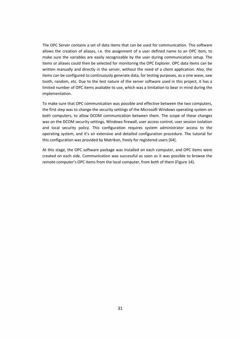
31
The OPC Server contains a set of data items that can be used for communication. This software
allows the creation of aliases, i.e. the assignment of a user defined name to an OPC item, to
make sure the variables are easily recognizable by the user during communication setup. The
items or aliases could then be selected for monitoring the OPC Explorer. OPC data items can be
written manually and directly in the server, without the need of a client application. Also, the
items can be configured to continuously generate data, for testing purposes, as a sine wave, saw
tooth, random, etc. Due to the test nature of the server software used in this project, it has a
limited number of OPC items available to use, which was a limitation to bear in mind during the
implementation.
To make sure that OPC communication was possible and effective between the two computers,
the first step was to change the security settings of the Microsoft Windows operating system on
both computers, to allow DCOM communication between them. The scope of these changes
was on the DCOM security settings, Windows firewall, user access control, user session isolation
and local security policy. This configuration requires system administrator access to the
operating system, and it’s an extensive and detailed configuration procedure. The tutorial for
this configuration was provided by Matrikon, freely for registered users [64].
At this stage, the OPC software package was installed on each computer, and OPC items were
created on each side. Communication was successful as soon as it was possible to browse the
remote computer’s OPC items from the local computer, from both of them (Figure 14).
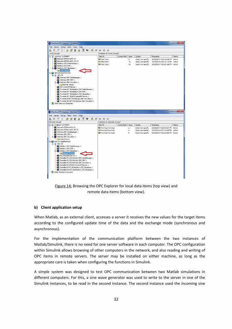
32
Figure 14: Browsing the OPC Explorer for local data items (top view) and
remote data items (bottom view).
b) Client application setup
When Matlab, as an external client, accesses a server it receives the new values for the target items
according to the configured update time of the data and the exchange mode (synchronous and
asynchronous).
For the implementation of the communication platform between the two instances of
Matlab/Simulink, there is no need for one server software in each computer. The OPC configuration
within Simulink allows browsing of other computers in the network, and also reading and writing of
OPC items in remote servers. The server may be installed on either machine, as long as the
appropriate care is taken when configuring the functions in Simulink.
A simple system was designed to test OPC communication between two Matlab simulations in
different computers. For this, a sine wave generator was used to write to the server in one of the
Simulink instances, to be read in the second instance. The second instance used the incoming sine
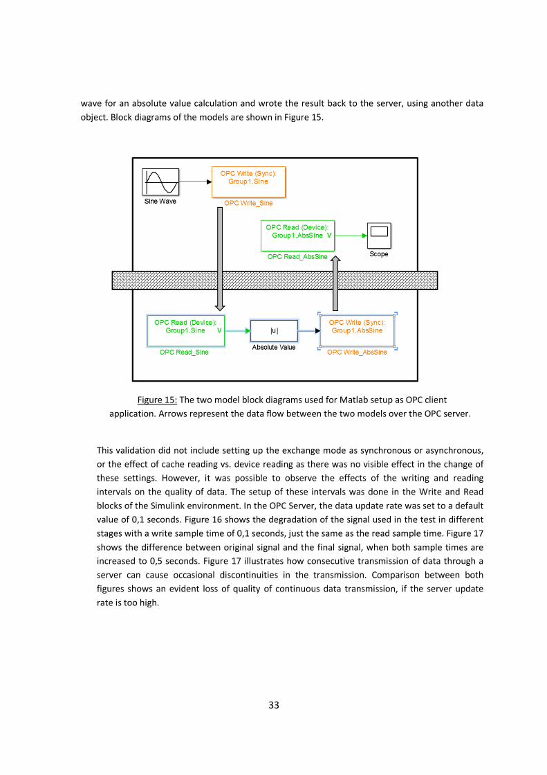
33
wave for an absolute value calculation and wrote the result back to the server, using another data
object. Block diagrams of the models are shown in Figure 15.
Figure 15: The two model block diagrams used for Matlab setup as OPC client
application. Arrows represent the data flow between the two models over the OPC server.
This validation did not include setting up the exchange mode as synchronous or asynchronous,
or the effect of cache reading vs. device reading as there was no visible effect in the change of
these settings. However, it was possible to observe the effects of the writing and reading
intervals on the quality of data. The setup of these intervals was done in the Write and Read
blocks of the Simulink environment. In the OPC Server, the data update rate was set to a default
value of 0,1 seconds. Figure 16 shows the degradation of the signal used in the test in different
stages with a write sample time of 0,1 seconds, just the same as the read sample time. Figure 17
shows the difference between original signal and the final signal, when both sample times are
increased to 0,5 seconds. Figure 17 illustrates how consecutive transmission of data through a
server can cause occasional discontinuities in the transmission. Comparison between both
figures shows an evident loss of quality of continuous data transmission, if the server update
rate is too high.
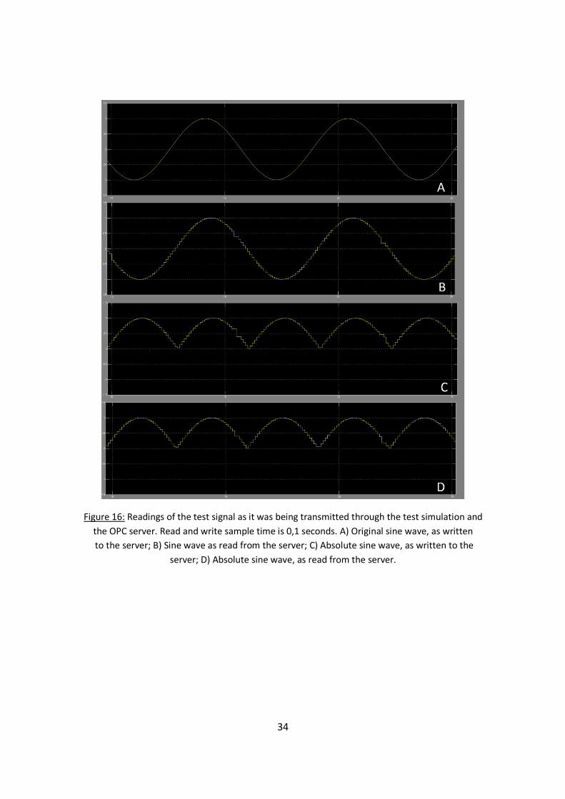
34
Figure 16: Readings of the test signal as it was being transmitted through the test simulation and
the OPC server. Read and write sample time is 0,1 seconds. A) Original sine wave, as written
to the server; B) Sine wave as read from the server; C) Absolute sine wave, as written to the
server; D) Absolute sine wave, as read from the server.
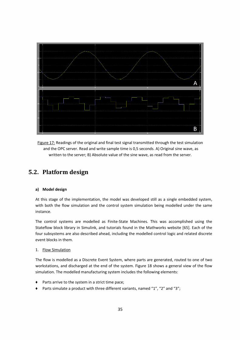
35
Figure 17: Readings of the original and final test signal transmitted through the test simulation
and the OPC server. Read and write sample time is 0,5 seconds. A) Original sine wave, as
written to the server; B) Absolute value of the sine wave, as read from the server.
5.2. Platform design
a) Model design
At this stage of the implementation, the model was developed still as a single embedded system,
with both the flow simulation and the control system simulation being modelled under the same
instance.
The control systems are modelled as Finite-State Machines. This was accomplished using the
Stateflow block library in Simulink, and tutorials found in the Mathworks website [65]. Each of the
four subsystems are also described ahead, including the modelled control logic and related discrete
event blocks in them.
1. Flow Simulation
The flow is modelled as a Discrete Event System, where parts are generated, routed to one of two
workstations, and discharged at the end of the system. Figure 18 shows a general view of the flow
simulation. The modelled manufacturing system includes the following elements:
♦ Parts arrive to the system in a strict time pace;
♦ Parts simulate a product with three different variants, named “1”, “2” and “3”;
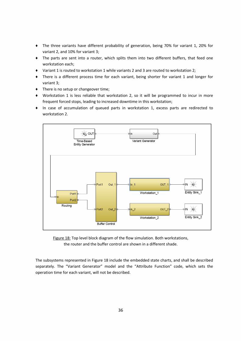
36
♦ The three variants have different probability of generation, being 70% for variant 1, 20% for
variant 2, and 10% for variant 3;
♦ The parts are sent into a router, which splits them into two different buffers, that feed one
workstation each;
♦ Variant 1 is routed to workstation 1 while variants 2 and 3 are routed to workstation 2;
♦ There is a different process time for each variant, being shorter for variant 1 and longer for
variant 3;
♦ There is no setup or changeover time;
♦ Workstation 1 is less reliable that workstation 2, so it will be programmed to incur in more
frequent forced stops, leading to increased downtime in this workstation;
♦ In case of accumulation of queued parts in workstation 1, excess parts are redirected to
workstation 2.
Figure 18: Top level block diagram of the flow simulation. Both workstations,
the router and the buffer control are shown in a different shade.
The subsystems represented in Figure 18 include the embedded state charts, and shall be described
separately. The “Variant Generator” model and the “Attribute Function” code, which sets the
operation time for each variant, will not be described.
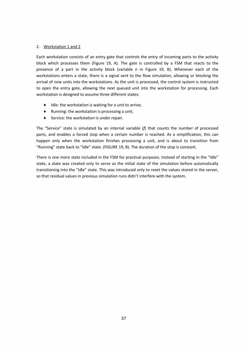
37
2. Workstation 1 and 2
Each workstation consists of an entry gate that controls the entry of incoming parts to the activity
block which processes them (Figure 19, A). The gate is controlled by a FSM that reacts to the
presence of a part in the activity block (variable n in Figure 19, B). Whenever each of the
workstations enters a state, there is a signal sent to the flow simulation, allowing or blocking the
arrival of new units into the workstations. As the unit is processed, the control system is instructed
to open the entry gate, allowing the next queued unit into the workstation for processing. Each
workstation is designed to assume three different states:
♦ Idle: the workstation is waiting for a unit to arrive;
♦ Running: the workstation is processing a unit;
♦ Service: the workstation is under repair.
The “Service” state is simulated by an internal variable (f) that counts the number of processed
parts, and enables a forced stop when a certain number is reached. As a simplification, this can
happen only when the workstation finishes processing a unit, and is about to transition from
“Running” state back to “Idle” state. (FIGURE 19, B). The duration of the stop is constant.
There is one more state included in the FSM for practical purposes. Instead of starting in the “Idle”
state, a state was created only to serve as the initial state of the simulation before automatically
transitioning into the “Idle” state. This was introduced only to reset the values stored in the server,
so that residual values in previous simulation runs didn’t interfere with the system.
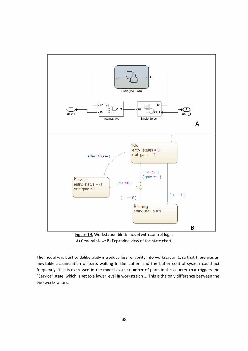
38
A
B Figure 19: Workstation block model with control logic.
A) General view; B) Expanded view of the state chart.
The model was built to deliberately introduce less reliability into workstation 1, so that there was an
inevitable accumulation of parts waiting in the buffer, and the buffer control system could act
frequently. This is expressed in the model as the number of parts in the counter that triggers the
“Service” state, which is set to a lower level in workstation 1. This is the only difference between the
two workstations.
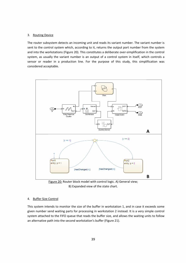
39
3. Routing Device
The router subsystem detects an incoming unit and reads its variant number. The variant number is
sent to the control system which, according to it, returns the output port number from the system
and into the workstations (Figure 20). This constitutes a deliberate over-simplification in the control
system, as usually the variant number is an output of a control system in itself, which controls a
sensor or reader in a production line. For the purpose of this study, this simplification was
considered acceptable.
A
B Figure 20: Router block model with control logic. A) General view;
B) Expanded view of the state chart.
4. Buffer Size Control
This system intends to monitor the size of the buffer in workstation 1, and in case it exceeds some
given number send waiting parts for processing in workstation 2 instead. It is a very simple control
system attached to the FIFO queue that reads the buffer size, and allows the waiting units to follow
an alternative path into the second workstation’s buffer (Figure 21).
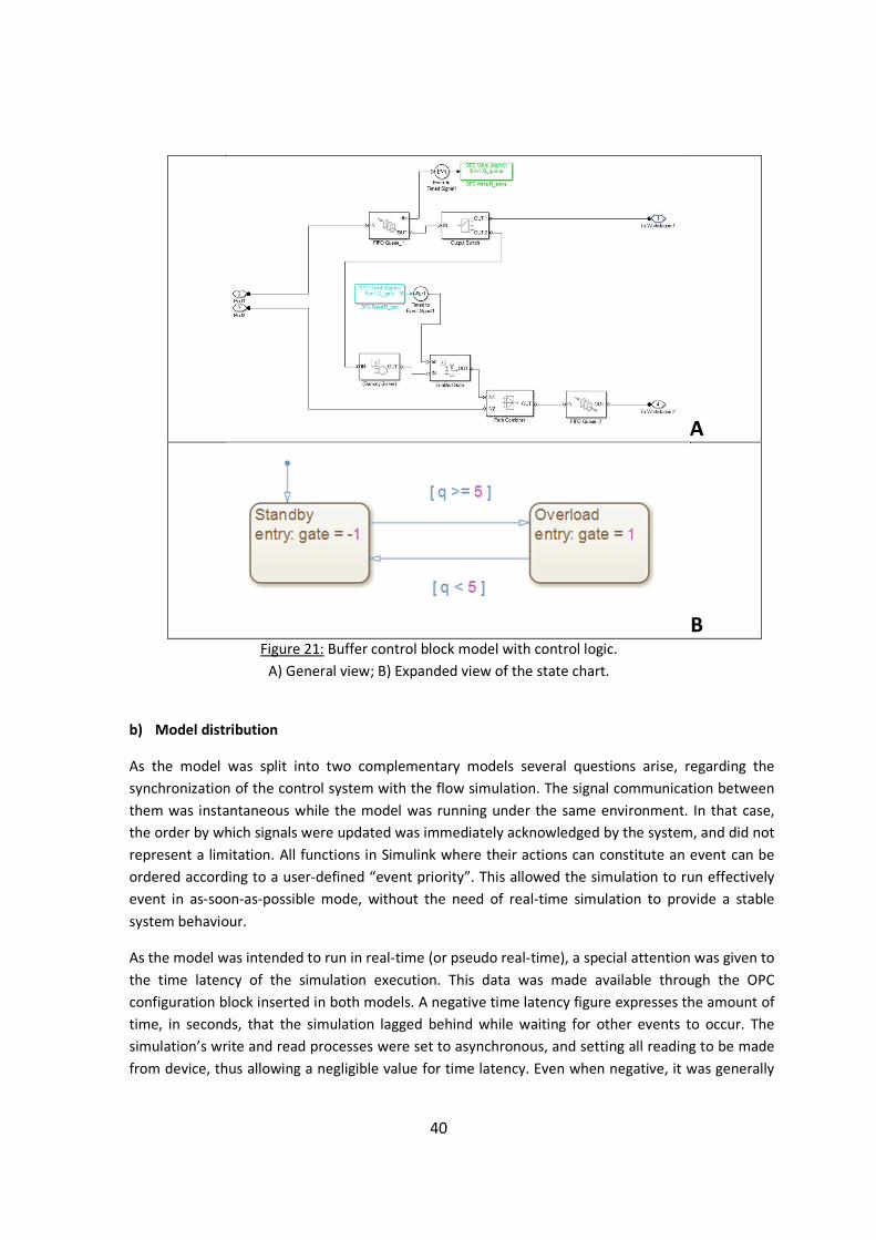
40
A
B Figure 21: Buffer control block model with control logic.
A) General view; B) Expanded view of the state chart.
b) Model distribution
As the model was split into two complementary models several questions arise, regarding the
synchronization of the control system with the flow simulation. The signal communication between
them was instantaneous while the model was running under the same environment. In that case,
the order by which signals were updated was immediately acknowledged by the system, and did not
represent a limitation. All functions in Simulink where their actions can constitute an event can be
ordered according to a user-defined “event priority”. This allowed the simulation to run effectively
event in as-soon-as-possible mode, without the need of real-time simulation to provide a stable
system behaviour.
As the model was intended to run in real-time (or pseudo real-time), a special attention was given to
the time latency of the simulation execution. This data was made available through the OPC
configuration block inserted in both models. A negative time latency figure expresses the amount of
time, in seconds, that the simulation lagged behind while waiting for other events to occur. The
simulation’s write and read processes were set to asynchronous, and setting all reading to be made
from device, thus allowing a negligible value for time latency. Even when negative, it was generally
41
under 0.01 seconds. As stated before, the only exception where synchronous communication was
set was the case where the order sequence had to be maintained. The router control system was
such a case, as will be described later in detail.
All data update time intervals were set to the minimum possible, both at the OPC server, the OPC
Read function blocks and the OPC Write function blocks. Nevertheless, it was not possible to
establish priority of reading and writing, so the order of these actions could be compromised and
had to be assured in a different way. This required some adaptations to the model, namely the
restriction to real-time execution and the introduction of changes into the model, to force the
system’s logic to respect an adequate sequence and to wait for some events to happen before
allowing other events to occur.
1. Flow Simulation
The configuration of the main flow simulation did not need any adjustment to run distributed, only
the control systems. Nevertheless, changes were made to the associated DES components inside the
respective subsystem that interact with the FSM. In the current implementation, only the FSM
charts are separated from the remaining model.
2. Workstation 1 and 2
Apart from the introduction of the OPC interface blocks, no other functional configuration change
was made in this step of the implementation.
3. Routing Device
The routing device model required introduction of more variables in the control system to
accomplish its function. The initial model dealt only with the incoming part’s counting number, the
part variant number and the returned output port number. To make sure the sequence of the
control logic was respected the whole FSM was rebuilt to accommodate more states, with clearer
distinction between the logical steps (Figure 22, B), and two other variables were introduced:
♦ An output count (d), allowing departure detection as a prerequisite for a new part to enter;
♦ A gate signal, to block the arriving part while waiting for value updates from the FSM.
These changes were introduced to prevent the arriving part to move through the system based on
outdated values. In short, the main purpose of the changes is to keep the flow simulation waiting
while the control logic is doing its part.
During the design of the control system of the routing device, a special attention was given to signal
update sequence. The values written to the OPC server are not specific to any event, so the variant
number, when written to the server, doesn’t carry a reference to the part it belongs to. The server
doesn’t have the capability of distinguishing the variant number of two different parts, if they
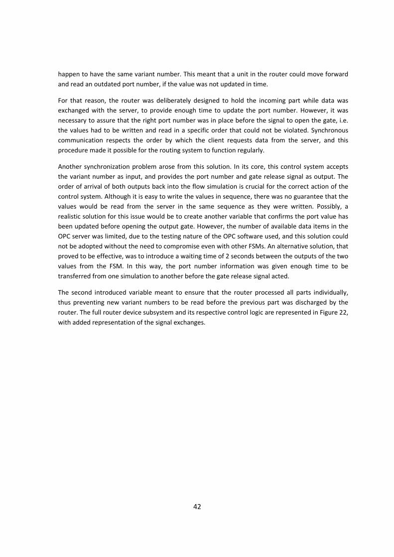
42
happen to have the same variant number. This meant that a unit in the router could move forward
and read an outdated port number, if the value was not updated in time.
For that reason, the router was deliberately designed to hold the incoming part while data was
exchanged with the server, to provide enough time to update the port number. However, it was
necessary to assure that the right port number was in place before the signal to open the gate, i.e.
the values had to be written and read in a specific order that could not be violated. Synchronous
communication respects the order by which the client requests data from the server, and this
procedure made it possible for the routing system to function regularly.
Another synchronization problem arose from this solution. In its core, this control system accepts
the variant number as input, and provides the port number and gate release signal as output. The
order of arrival of both outputs back into the flow simulation is crucial for the correct action of the
control system. Although it is easy to write the values in sequence, there was no guarantee that the
values would be read from the server in the same sequence as they were written. Possibly, a
realistic solution for this issue would be to create another variable that confirms the port value has
been updated before opening the output gate. However, the number of available data items in the
OPC server was limited, due to the testing nature of the OPC software used, and this solution could
not be adopted without the need to compromise even with other FSMs. An alternative solution, that
proved to be effective, was to introduce a waiting time of 2 seconds between the outputs of the two
values from the FSM. In this way, the port number information was given enough time to be
transferred from one simulation to another before the gate release signal acted.
The second introduced variable meant to ensure that the router processed all parts individually,
thus preventing new variant numbers to be read before the previous part was discharged by the
router. The full router device subsystem and its respective control logic are represented in Figure 22,
with added representation of the signal exchanges.
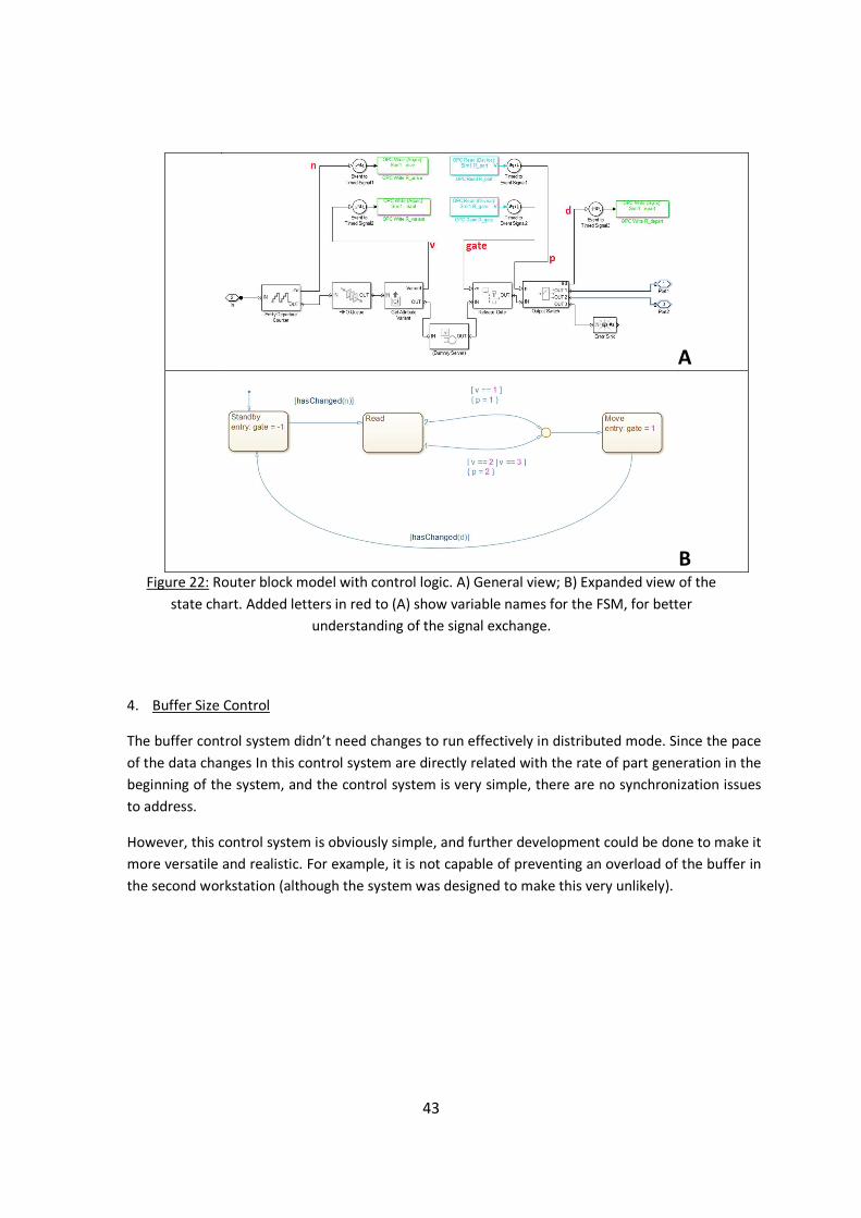
43
A
B Figure 22: Router block model with control logic. A) General view; B) Expanded view of the
state chart. Added letters in red to (A) show variable names for the FSM, for better
understanding of the signal exchange.
4. Buffer Size Control
The buffer control system didn’t need changes to run effectively in distributed mode. Since the pace
of the data changes In this control system are directly related with the rate of part generation in the
beginning of the system, and the control system is very simple, there are no synchronization issues
to address.
However, this control system is obviously simple, and further development could be done to make it
more versatile and realistic. For example, it is not capable of preventing an overload of the buffer in
the second workstation (although the system was designed to make this very unlikely).
44
Chapter 6
Conclusion
6.1. Discussion
Communication configuration
DCOM communication poses two threats to implementation in business environment. First, it required
deactivation of most Windows security features, such as firewalls and anti-virus software. Furthermore,
all OPC software required administrator privileges to execute. According to the server’s vendor website
[66] such problems may be solved using an OPC tunnelling software , i.e. encapsulating the exchanged
data in a different communication protocol to be safely transmitted through a network, without directly
using DCOM.
Second, DCOM communication technology works best in environments with low latency and high
bandwidth. The proposed platform was configured in only two computers connected with a network
switch. This allowed DCOM communication technology to work in its optimal performance setting.
Considerable difficulty may be found when communicating over bandwidth limited communication
devices.
Due to the testing purpose of the OPC server software, there was a limit to the number of OPC items
available for data exchange. This limitation had impact on the simulation model design, since the control
system models couldn’t be developed to a very complex level, and the number of control systems that
could run simultaneously was also hindered by this. However, the modelled system was enough to
provide good perspectives on the utilization of this communication architecture for a distributed
simulation platform.
If the control logic being developed isn’t meant to be deployed into a PLC, i.e. the computer is the
intended running environment of the control system, it can be important from the perspective of the
developer to work with two simulations that interact using the same technology as the reality being
modelled. In this way, it is possible to expose the overall behaviour of the networked system, which may
not be possible when simulating either the control or the communication system separately. Therefore,
it may become possible to study how the network topology, medium access, routing protocols and the
traffic pattern affect the overall control system performance [36].
45
During the implementation, in each of the three steps, it was necessary to adjust the model. The three
steps of implementation correspond to three increasing levels of separation between the flow
simulation and the control system. Consequently, the delay associated to the writing and reading of
data through the server increased. This delay is negligible within the same simulation environment, but
becomes significant when communicating through a server, and even more when communicating
between different computers.
Simulation Platform Development
The final result of this thesis is a manufacturing system simulation where the flow simulation and the
control system run in separate machines. The purpose of the parallel simulation platform was
accomplished even during the implementation work. There was much troubleshooting being made to
overcome update rate issues which was done with the systems running in parallel, and allowing the
changes to be validated promptly and effectively. It was also possible to evaluate several design
alternatives and explore scenarios using different simulation parameters.
Although the initial purpose was to use ExtendSim [45] for the flow simulation, there could be a great
advantage in using Simulink instead. Simulink is a very broad simulation tool, very versatile for a lower
level of simulation and signal based modelling. Although there are simulation blocks in Simulink for
common DES functions, these blocks could not always be used in the distributed simulation. Specifically,
the routing device had to be broken down and built with several simple functions, in order to be split
into two different systems, and this increased the demanded level of detail from the simulation model.
This made Matlab/Simulink a very useful tool, but it is uncertain if the same could be accomplished with
ExtendSim. Nevertheless, Matlab/Simulink is not generally meant for modelling of finite variables, the
interface allow less visibility of finite entities and that made model troubleshooting a slightly harder
task.
The modelling of the distributed simulation was different from the real life application of control
systems. Indeed, control systems logic usually operates between sensors and actuators in a
manufacturing cell, and the model used in this project was a global over-simplified flow simulation.
However, there was some abstraction required since all communication had to be done with signals and
values, and instructions had to be converted into numerical form to be written to the server. Also, since
control signals and values were generated remotely and read from a server, they were not destined to a
specific entity in the flow simulation. Therefore, there was a good approximation to control system
development, and the simulation platform proved to be useful for the purpose.
The communication between the two systems found its main limitation in the capacity to update the
data signals from the control system to the flow simulation, while respecting the event order that allows
the control system to be effective. These limitations raise the awareness for the order in which the
instructions are sent from the control system to the server and to other client applications. The
simulation model used for the router clearly shows an example of a system where the order of two
signal updates is fundamental for the system to work as intended. Considering the scope and the
46
limitations of this thesis, this synchronization issue was addressed by setting up different data exchange
modes (synchronous/asynchronous) to different logical processes in the simulation, in order to achieve
a compromise between event ordering and execution latency.
While the control system was being developed under the same simulation environment as the flow
simulation this effect was masked, as the system works well when the two signals are updated
simultaneously. A slower communication may offer a better opportunity for debugging but will not
relate to the challenges that exist if the control logic is coded and deployed into a PLC. PLC code and
infrastructure bears less communication overhead and is generally faster than the state machine
running on a computer, so this problem is very unlikely to exist in the real-life control system
The use of FSM to model control systems proved very practical to understand control system logic, even
without prior knowledge. Due to its graphical and intuitive form, it’s possible to observe the state
machine operating in real-time, and it’s easy to debug the model immediately.
Simulation Platform Execution
The connected models were successfully executed in parallel. This corresponds to a successful division
of the control model suggested by the literature [5], into the flow model and the control logic (Figure 1).
This component of the framework was already functionally divided, since it required two different
development engineers to work on each part. This implementation contributes with a possibility of
physical division of the model in two, allowing separate and concurrent development. This translates
into the possibility of quick validation and troubleshooting of the simulation models, as well as testing
different simulation parameters and design alternatives. The full control model is suitable to be
connected to a virtual cell model, according to the Virtual Commissioning implementations present in
the literature [5] [16] [67].
The platform’s main limitation is that it’s not possible to change the model while the simulation was
running, and the only possible user interaction in run-time is data observation. The debugging process
always required the system to be stopped and re-started. For that reason, the system presented cannot
be considered a virtual environment, but a distributed analytic simulation [33]. In practice, usage of the
system for development requires the two developers to start their side of the simulation separately, so
some coordination and communication is still required. However, the developed platform allows control
system developers to start working before the flow development is completely finalized, so the
framework for concurrent development is achieved.
The two systems worked in parallel, i.e. the flow simulation halted while waiting for the control system
to return a signal. Real-time execution was necessary for this to happen and the data writing and
reading was made asynchronously to avoid latency. However, industrial control often requires a certain
sequence of instructions to be respected, which is not possible with asynchronous communication.
Therefore, synchronous communication should be used only in the cases where strictly necessary.
47
Since the platform was forcefully run in real-time, and not in as-fast-as-possible mode, the simulation
time is inevitably increased. This effect may counterbalance the time saving from applying the principles
of concurrent engineering to this development stage.
6.2. Future Work
This thesis was limited to the concurrent development of the industrial flow with the control system. A
relevant expansion of this method would be to implement a holistic distributed Virtual Commissioning
system, by including the automatic generation of PLC code in Matlab. This can be accomplished by
considering the model proposed in the literature [2] for the deployment and validation of the control
code.
In this thesis, a single Discrete Event System was coupled to a single simulation of multiple independent
Finite State Machines. This simulation was running on two computers, but the same method could be
applied to connect more machines in the same network and allow the multiple control systems to be
developed in different computers by different developers. Furthermore, it is possible to split the flow
simulation itself into different machines, and distribute the development of the DES alone by different
developers, as in the modular development of manufacturing systems proposed in the literature [3].
However, it should be noted that using synchronous communication with a larger amount of data
objects may increase simulation latency.
Due to the testing purpose of the OPC server used, the number of OPC items available is limited, since
it’s a freeware product designed for simulation purposes. The use of more items can be possible with
full commercial versions, although the required investment was inappropriate for the nature of the
thesis. Other software packages can be used, perhaps also for free, with more available items which
would increase the quality of the control systems.
The model used for this simulation platform was very simple and generic. Considering the successful
application of the platform in this case, the next natural step is to model an actual manufacturing cell
with robots, conveyors and machines, where this methodology could be used to save development
time.
Although Matlab/Simulink is considered adequate for development of control systems, there may be
other simulation environments more appropriate for factory flow simulation using DES. The use of
ExtendSim could be made possible if newer versions include OPC interface, or the OPC write and read
functions could be coded in the software’s proprietary language (ModL/C++). Alternatively, the existing
DDE interface of ExtendSim could be explored, although being a legacy technology.
48
Chapter 5
References
[1] Cen, M. ; Liu, Q. ; Yan, Y. (2012) OPC (OLE for Process Control) based Calibration System for
Embedded Controller. Journal of Software, vol.7, no.12.
[2] Andemeskel, F. (2013) Model-based Virtual Commissioning of a Manufacturing Cell Control
System. Degree Project in Production Engineering Management. KTH – The Royal Institute of
Technology. Stockholm, Sweden.
[3] Olofsgård, P. ; Ng, A. ; Moore, P. ; Pu, J. ; Wong, C.B. ; De Vin, L. (2002) Distributed Virtual
Manufacturing for Development of Modular Machine Systems. Journal of Advanced
Manufacturing Systems. Vol.1, no.2, pp.141-158.
[4] Makris, S. ; Michalos, G. ; Chryssolouris, G. (2012) Virtual Commissioning of an Assembly Cell
with Cooperating Robots. Advances in Decision Sciences. Vol.2012, ID 428060.
[5] Hossain, M. ; Semere, D.T. (2013) Virtual Control System Development Platform with the
Application of PLC Device. Proceeding of the International MultiConference of Engineers and
Computer Scientists 2013. Vol.II.
[6] Pelliciari, M. ; Andrisano, A.O. (2009) Engineering method for adaptive manufacturing systems
design. International Journal on Interactive Design and Manufacturing. No.3, pp.81-91.
[7] Neugebauer, R. ; Schob, U. (2011) Reducing the model generation effort for the virtual
commissioning of control programs. Production Engineering. Vol.5, no.5, pp.539-547.
[8] Aganovic, D. (2004) On Manufacturing System Development in the Context of Concurrent
Engineering. Doctoral thesis. KTH – Royal Institute of Technology, Department of Production
Engineering. Stockholm, Sweden.
[9] Pullan, T.T. ; Bhasi, M. ; Madhu, G. (2014) Application of concurrent engineering in
manufacturing industry.International Journal of Computer Integrated Manufacturing. Vol.23,
no.5, pp.425-440.
[10] Yetukuri, B.N. ; Yetukuri, N.V. ; Fischer, G.W. (1996) SPAW: A design tool for planning a
manufacturing process in a concurrent engineering environment. Computers in Industry. No.32,
pp.79-93.
[11] Nategh, M.J. (2009) Concurrent engineering planning on the basis of forward and backward
effects of manufacturing processes. International Journal of Production Research. Vol.47, no.18,
p.5147-5161.
49
[12] Mandić, V. ; Erić, D. ; Adamović, D. ; Janjić, M. ; Jurković, Z. ; Babić, Z. ; Ćosić, P. () Concurrent
engineering based on virtual manufacturing. Tehnićki Vjesnik (Technical Gazette). Vol.19, no.4,
pp.885-892.
[13] Sun, J. ; Zhang, Y.F. ; Nee, A.Y.C. (2001) A distributed multi-agent environment for product
design and manufacturing planning. International Journal of Production Research. Vol.39, no.4,
pp.625-645.
[14] Shahin, A. ; Rostamian, N. (2013) Concurrent engineering and manufacturing flexibility: an
integrated model. International Journal of Productivity and Quality Management. Vol.12, no.2,
pp.121-140.
[15] Valle, S. ; Vásquez-Bustelo, D. (2009) Concurrent engineering performance: Incremental versus
radical innovation. International Journal of Production Economics. No.119, pp.136-148.
[16] Hoffmann, P. ; Maksoud, T.M.A. (2010) Virtual commissioning of manufacturing systems – A
review and new approaches for simplification. Proceedings of the 24th European Conference on
Modelling and Simulation, ECMS 2010, pp.175 -181
[17] Hespanha, J.P. ; Naghshtabrizi, P. ; Xu,, Y. (2007) A survey of recent results in Networked Control
Systems. Proceedings of the IEEE, Vol.95, no.1, pp.138-162.
[18] Antsakis, P. ; Baillieul, J. (2007) Special Issue on Technology of Networked Control Systems.
Proceedings of the IEEE. Vol.95, no.1.
[19] Galloway, B. ; Hancke, G.P. (2013) Introduction to Industrial Control Networks. IEEE
Communications, Surveys and Tutorials, Vol. 15, no. 2.
[20] Mahnke, W.; Leitner, S.;Damm, M. (2009) OPC Unified Architecture. Springer-Verlag Berlin
Heidelberg.
[21] Şahin, C. ; Bolat, E.D. (2009) Development of remote control and monitoring of web-based
distributed OPC system. Computer Standards and Interfaces. No.31, pp.984-993
[22] Silvente, J. ; Monroy, I. ; Escudero, G. ; Espuña, A. ; Graells, M. (2012) A promising OPC-based
computer system applied to fault diagnosis. Proceeding of the 22nd European Symposium in
Computer Aided Process Engineering.
[23] Tan, V.V. ; Yoo, D.S. ; Yi, M.J. (2008) A Multiagent-System Framework for Hierarchical Control
and Monitoring of Complex Process Control Systems. Chapter of PRIMA 2008, LNAI 5357, pp.
381-388. (2008) Springer-Verlag Berlin Heidelberg.
[24] Lieping, Z. ; Aiqun, Z. ; Yunsheng, Z. (2007) On Remote Real-time Communication between
Matlab and PLC based on OPC Technology. Proceedings of the 26th Chinese Control Conference.
[25] Alves Santos, R. ; Normey-Rico, J.E. ; Merino Gómez, A. ; Acebes Arconada, L.F. ; Prada Moraga,
C. (2005) OPC based distributed real time simulation of complex continuous processes.
Simulation Modelling Practice and Theory. No.13, pp.525-549.
50
[26] Hong, X. ; Jianhua, W. (2006) Using standard components in automation industry: A study on
OPC specification. Computer Standards & Interfaces. No.28, pp.386-395.
[27] https://opcfoundation.org/about/opc-technologies/opc-ua, visited 23/07/2014.
[28] http://www.microsoft.com/com, visited 28/07/2014.
[29] Huang, Q. ; Song, S. (2009) Real-time Control System Based on MATLAB and PCAuto via OPC
technology. Proceeding of the IEEE International Conference on Intelligent Computing and
Intelligent Systems – ICIS 2009. Vol.2, pp.671-674.
[30] Sabin Diaz, D. ; De Keyser, R. (2011) WinCC Application via OPC Communication to MatLab for
Integrated Systems. IEEE International Conference on Emerging Technologies and Factory
Automation - ETFA’2011.
[31] Taneva, A. ; Muskinja, N. ; Petrov, M. ; Tovornik, B. (2004) FPID Controller: Real Time
Application. Second IEEE International Conference on Intelligent Systems.
[32] Perumalla, K.S. (2006) Parallel and distributed simulation: Traditional techniques and recent
advances. Proceedings of the 2006 Winter Simulation Conference.
[33] Fujimoto, R.M. (2000) Parallel and Distributed Simulation Systems. John Wiley & Sons, Canada.
[34] Hoseyni-Nasab, M. ; Andradóttir, S. (1998) Time segmentation parallel simulation of tandem
queues with manufacturing blocking. Proceedings of the 1998 Winter Simulation Conference.
[35] Roy, R. ; Arunachalam, R. (2004) Parallel discrete event simulation algorithm for manufacturing
supply chains. Journal of the Operational Research Society. No.55, pp.622-629.
[36] Li, W. ; Zhang, X. ; Li, H. (2014) Co-simulation platforms for co-design of networked control
systems: An Overview. Control Engineering Practice, No.23, pp.44-56.
[37] Cassandras, C.G. (2005) Discrete-Event Systems in Handbook of Networked and Embedded
Control Systems. Hristu-Varsakelis, D.; Levine, W.S. (Editors). Birkhäuser Boston.
[38] Cigolini, R. ; Pero, M. ; Rossi, T. ; Sianesi, A. (2014) Linking supply chain configuration to supply
chain performance: A discrete event simulation model. Simulation Modelling Practice and
Theory. No.40, pp.1–11.
[39] Cassandras, C.G. , Lafortune, S. (2008) Introduction to Discrete Event Systems. Second Edition.
Springer Science+Business Media LLC, New York, USA.
[40] Negahban, A. ; Smith, J.S. (2014) Simulation for manufacturing system design and operation:
Literature review and analysis. Journal of Manufacturing Systems. Article in press.
[41] Skoogh, A. ; Perera, T. ; Johansson, B. (2012) Input data management in simulation - Industrial
Practices and Future Trends. Simulation Modelling Practice and Theory. No.29, pp.181-192.
[42] Shararah, M.A. ; El-Kilany, K.S. ; El-Sayed, A.E. (2011) Value Stream Map Simulator Using
ExtendSim. Proceedings of the World Congress on Engineering (WCE 2011). Vol.I.
51
[43] Zimmerman, A. (2008) Stochastic Discrete Event Systems – Modeling, Evaluation, Applications.
Springer-Verlag, Berlin/Heidelberg.
[44] http://www.mathworks.se/discrete-event-simulation, visited 17/09/2014.
[45] http://www.extendsim.com , visited 17/09/2014.
[46] https://www.arenasimulation.com, visited 17/09/2014.
[47] Kruth, J.P. ; Van Ginderachter, T. ; Tanaya, P.I. ; Valckenaers, P. (2001) The use of finite state
machines for task-based machine tool control. Computers in Industry. No.46, pp.247-258.
[48] Lawson, M.V. (2005) Finite Automata in Handbook of Networked and Embedded Control
Systems. Hristu-Varsakelis, D.; Levine, W.S. (Editors). Birkhäuser Boston.
[49] Lee, D. ; Yannakakis, M. (1996) Principles and Methods of Testing Finite State Machines - A
Survey. Proceedings of the IEEE, Vol.84, no.8, pp.1090-1123.
[50] Hanžič, F. ; Jezernik, K. (2012) Finite-state machine control of mechatronic systems. Journal of
Systems and Control Engineering. Vol.226, no.10, pp.1394–1409.
[51] Wagner, F. ; Schmuki, R. ; Wagner, T. ; Wolstenholme, P. (2006) Modeling Software with Finite
State Machines - A Practical Approach. Taylor & Francis Group. Boca Raton, FL, USA.
[52] Yasuda, G. (2010) Implementation of Hierarchical and Distributed Control for discrete event
robotic manufacturing systems. Journal of Software Engineering & Applications. No.3, pp.436-
445.
[53] http://www.mathworks.se/discovery/finite-state-machine.html, visited 02/06/2014.
[54] http://www.mathworks.se/products/sl-plc-coder, visited 06/10/2014.
[55] Hu, X. (2012) FSM Models for Cell Control Code Generation (KTH). Degree Project in Production
Engineering Management, Second Level; 530. KTH, School of Industrial Engineering and
Management (ITM), Production Engineering.
[56] Le, C.V. ; Pang, C.K. ; Gan, O.P. ; Chee, X.M. ; Zhang, D.H. ; Luo, M. ; Chan, H.L. ; Lewis, F.L. (2012)
Classification of energy consumption patterns for energy audit and machine scheduling in
industrial manufacturing systems. Transactions of the Institute of Measurement and Control.
Vol.35, no.5, pp. 583–592.
[57] Endsley, E.W. ; Almeida, E.E. ; Tilbury, D.M. (2006) Modular finite state machines: Development
and application to reconfigurable manufacturing cell controller generation. Control Engineering
Practice. No.14, pp.1127–1142.
[58] Abdoli, S. (2013) A holistic machining line behavior modeling using Finite State Machines.
Degree Project in Production Engineering Management, Second Level; 585. KTH, School of
Industrial Engineering and Management (ITM), Production Engineering.
[59] Jamhour, A.; Garcia, C. (2012) Automation of industrial serial processes based on finite state
machines. Procedia Engineering. No.42, pp.186 – 196.
52
[60] Angluin, D. ; Aspnes, J. ; Barbosa Vargas, R. (2013) Mutation Systems. International Journal of
Computer Mathematics. Vol.90, no.6, pp.1132–1149.
[61] Gao, R. (2013) The Application of Finite State Machine in Modeling and Control of Gene
Mutation Process. IEEE Transactions on Nanobioscience. Vol.12, no.4, pp.265-274.
[62] Sitaula, C. ; Ojha, Y.R. (2013) Semantic Sentence Similarity Using Finite State Machine. Intelligent
Information Management, No.5, pp.171-174.
[63] Sales, D.O. ; Correa, D.O. ; Fernandes, L.C. ; Wolf, D.F. ; Osório, F.S. (2014) Adaptive finite state
machine based visual autonomous navigation system. Engineering Applications of Artificial
Intelligence. Vol.29, pp.152-162.
[64] http://www.matrikonopc.com, visited 19/04/2014.
[65] http://www.mathworks.se/help/stateflow/getting-started.html, visited 24/03/2014.
[66] http://www.matrikonopc.com/products/opc-data-management/opc-tunneller.aspx, visited
04/06/2014.
[67] Ko, M. ; Anh, E. ; Park, S.C. (2013) A concurrent design methodology of a production system for
virtual commissioning. Concurrent Engineering: Research and Applications. Vol.21, no. 2, pp.129-
140.
Recommended