MAXIMUM POWER POINT TRACKING FOR PHOTOVOLTAIC OPTIMIZATIONUSING EXTREMUM SEEKING

Steven L. Brunton1, Clarence W. Rowley1, Sanjeev R. Kulkarni1, and Charles Clarkson2

1Princeton University, Princeton, NJ 085442ITT Space Systems Division, Rochester, NY 14606

ABSTRACT

This work develops a maximum power point tracking (MPPT)algorithm for optimizing solar array performance that is robustto rapidly varying weather conditions. In particular, a novelextremum seeking (ES) controller, which utilizes the inverterripple, is designed and tested on a simulated array withgrid-tied inverter. The new algorithm is benchmarked againstthe perturb and observe (PO) method using irradiance datagathered on a rooftop array experiment in Princeton, NJ. Theextremum seeking controller achieves an efficiency of 99.7%and transient rise to the MPP of .1 seconds, which is 100 timesfaster than perturb and observe.

INTRODUCTION

Solar power is at the forefront of clean, renewable energy,and it is gaining momentum due to advances in solar panelmanufacturing and efficiency as well as increasingly volatilefuel costs. Photovoltaic (PV) solar cells are the most readilyavailable solar technology, and they operate best on brightdays with little or no obstruction to incident sunlight. However,frequent overcast days and partial obstructions such as treelimbs or buildings limit the reliability of solar power in much ofthe United States.

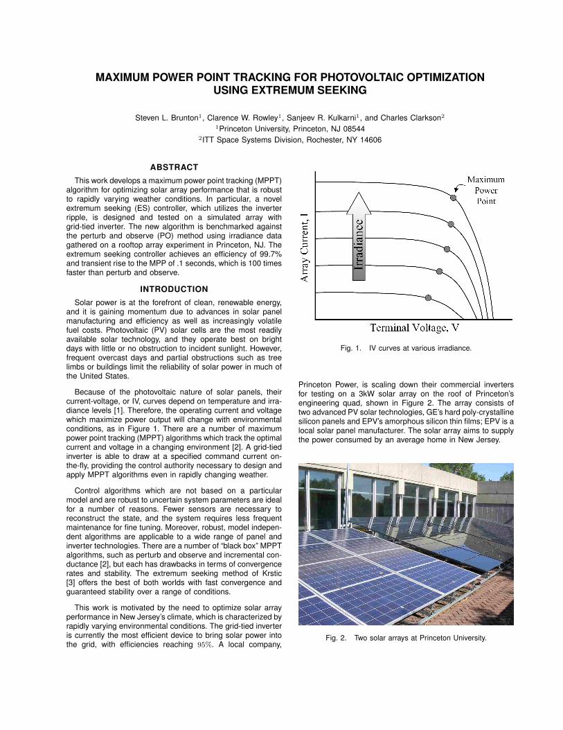
Because of the photovoltaic nature of solar panels, theircurrent-voltage, or IV, curves depend on temperature and irra-diance levels [1]. Therefore, the operating current and voltagewhich maximize power output will change with environmentalconditions, as in Figure 1. There are a number of maximumpower point tracking (MPPT) algorithms which track the optimalcurrent and voltage in a changing environment [2]. A grid-tiedinverter is able to draw at a specified command current on-the-fly, providing the control authority necessary to design andapply MPPT algorithms even in rapidly changing weather.

Control algorithms which are not based on a particularmodel and are robust to uncertain system parameters are idealfor a number of reasons. Fewer sensors are necessary toreconstruct the state, and the system requires less frequentmaintenance for fine tuning. Moreover, robust, model indepen-dent algorithms are applicable to a wide range of panel andinverter technologies. There are a number of “black box” MPPTalgorithms, such as perturb and observe and incremental con-ductance [2], but each has drawbacks in terms of convergencerates and stability. The extremum seeking method of Krstic[3] offers the best of both worlds with fast convergence andguaranteed stability over a range of conditions.

This work is motivated by the need to optimize solar arrayperformance in New Jersey’s climate, which is characterized byrapidly varying environmental conditions. The grid-tied inverteris currently the most efficient device to bring solar power intothe grid, with efficiencies reaching 95%. A local company,

Fig. 1. IV curves at various irradiance.

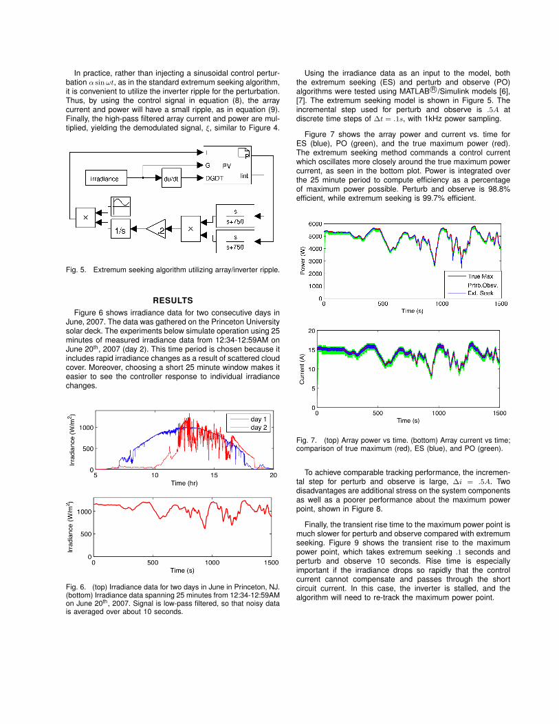
Princeton Power, is scaling down their commercial invertersfor testing on a 3kW solar array on the roof of Princeton’sengineering quad, shown in Figure 2. The array consists oftwo advanced PV solar technologies, GE’s hard poly-crystallinesilicon panels and EPV’s amorphous silicon thin films; EPV is alocal solar panel manufacturer. The solar array aims to supplythe power consumed by an average home in New Jersey.

Fig. 2. Two solar arrays at Princeton University.

PV ARRAY INVERTER MODEL

Figure 3 is a schematic of the array-inverter system.

PV Array uC

L

iv

Fig. 3. Schematic of PV array and inverter with LC dynamics.

Kirchoff’s law yields the following relationships:

i = u+ iC (1)vC = −v − vL (2)

The array IV curve has the form v = f(i, G), where G isirradiance, so equation (2) becomes:

vC = −f(i, G)− Ldi

dt(3)

=⇒ −dvC

dt=

d

dtf(i, G) + L

d2i

dt2(4)

=∂f(i, G)

∂i

di

dt+∂f(i, G)

∂G

dG

dt+ L

d2i

dt2(5)

Equation (1) and the capacitor equation yield:

dvC

dt=iC

C=⇒

dvC

dt= −

1

C(u− i) (6)

Combining equations (5) & (6) yields the system dynamicsin terms of inverter control current u and array current i:

LCd2i

dt2+ C

∂f

∂i

di

dt+ i = u− C

∂f

∂G

dG

dt(7)

The dynamical system given by equation (7) representsa forced oscillator with nonlinear damping. The forcing cor-responds to the inverter control current u as well as thechange in IV curve due to irradiance change, given by−C(∂f/∂G)(dG/dt).

To flow 60Hz AC power into the grid at a given currentu, the inverter switches DC current out of a large capacitor.This requires the following inverter control current with a large120Hz oscillation:

u = u (1 + sin(120× 2πt)) (8)

In practice, the LC circuit acts as a low pass filter betweenthe control current u, and the array current i, so that i experi-ences a 120Hz ripple at approximately 3% magnitude:

i ≈ u (1 + .03 sin(120× 2πt+ ϕ)) (9)

For more information on DC-AC power inverters, see Bose [4].

There is also a high frequency ripple at 20kHz due to theinverter sampling time; however, this is a small effect and isnot modeled.

The array IV curve v = f(i, G) is modeled using the lighted-diode equations [1], [5]:

I = IL − IOS

»exp

q

AkBT(V + IR)− 1

–(10)

IOS = IOR

„T

TR

«exp

„qEG

AkB

„1

TR−

1

R

««(11)

IL =G

1000(ISC +KT,I(T − TR)) (12)

V =AkBT

qln

„IL − IIOS

+ 1

«− IR (13)

where I and V are the same as i, v in Figure 3, IL is the lightgenerated current, IOS is the cell reverse saturation current,and T is temperature.

Values and definitions for other terms in the equations areas follows: TR = 298 (reference temperature), IOR = 2.25e− 6

(reverse saturation current at T = TR), ISC = 3.2 (short-circuitcurrent), EG = 1.8e − 19 (Silicon band gap), A = 1.6 (idealityfactor), kB = 1.38e− 23 (Boltzmann’s constant), q = 1.6e− 19

(electronic charge), R = .01 (resistance), and KT,I = .8 (short-circuit current temperature coefficient). Finally, the model arrayconsists of 3 parallel strings, each with 7 panels connectedin series. Each panel produces approximately 220W at fullirradiance, G = 1000 W/m2.

MAXIMUM POWER POINT TRACKING

Currently the most popular MPPT algorithm is perturb andobserve (PO), where the current is repeatedly perturbed by afixed amount in a given direction, and the direction is changedonly if the algorithm detects a drop in power between steps.Although this algorithm benefits from simplicity, it lacks thespeed and adaptability necessary for tracking fast transientsin weather.

A robust new maximum power point tracking algorithmis based on the extremum seeking (ES) control method. Aschematic of the algorithm is shown in Figure 4. This controllerconverges at a rate which is proportional to the slope of thePI curve and has guaranteed stability over a range of systemparameters [3].

Solar Array &Inverter Hardware

ss+!h

"s !+

current power

high-pass lter

integrator

!"

# sin $t

u

Fig. 4. Extremum seeking algorithm.

In practice, rather than injecting a sinusoidal control pertur-bation α sinωt, as in the standard extremum seeking algorithm,it is convenient to utilize the inverter ripple for the perturbation.Thus, by using the control signal in equation (8), the arraycurrent and power will have a small ripple, as in equation (9).Finally, the high-pass filtered array current and power are mul-tiplied, yielding the demodulated signal, ξ, similar to Figure 4.

Fig. 5. Extremum seeking algorithm utilizing array/inverter ripple.

RESULTSFigure 6 shows irradiance data for two consecutive days in

June, 2007. The data was gathered on the Princeton Universitysolar deck. The experiments below simulate operation using 25minutes of measured irradiance data from 12:34-12:59AM onJune 20th, 2007 (day 2). This time period is chosen because itincludes rapid irradiance changes as a result of scattered cloudcover. Moreover, choosing a short 25 minute window makes iteasier to see the controller response to individual irradiancechanges.

Fig. 6. (top) Irradiance data for two days in June in Princeton, NJ.(bottom) Irradiance data spanning 25 minutes from 12:34-12:59AMon June 20th, 2007. Signal is low-pass filtered, so that noisy datais averaged over about 10 seconds.

Using the irradiance data as an input to the model, boththe extremum seeking (ES) and perturb and observe (PO)algorithms were tested using MATLAB R©/Simulink models [6],[7]. The extremum seeking model is shown in Figure 5. Theincremental step used for perturb and observe is .5A atdiscrete time steps of ∆t = .1s, with 1kHz power sampling.

Figure 7 shows the array power and current vs. time forES (blue), PO (green), and the true maximum power (red).The extremum seeking method commands a control currentwhich oscillates more closely around the true maximum powercurrent, as seen in the bottom plot. Power is integrated overthe 25 minute period to compute efficiency as a percentageof maximum power possible. Perturb and observe is 98.8%efficient, while extremum seeking is 99.7% efficient.

Fig. 7. (top) Array power vs time. (bottom) Array current vs time;comparison of true maximum (red), ES (blue), and PO (green).

To achieve comparable tracking performance, the incremen-tal step for perturb and observe is large, ∆i = .5A. Twodisadvantages are additional stress on the system componentsas well as a poorer performance about the maximum powerpoint, shown in Figure 8.

Finally, the transient rise time to the maximum power point ismuch slower for perturb and observe compared with extremumseeking. Figure 9 shows the transient rise to the maximumpower point, which takes extremum seeking .1 seconds andperturb and observe 10 seconds. Rise time is especiallyimportant if the irradiance drops so rapidly that the controlcurrent cannot compensate and passes through the shortcircuit current. In this case, the inverter is stalled, and thealgorithm will need to re-track the maximum power point.

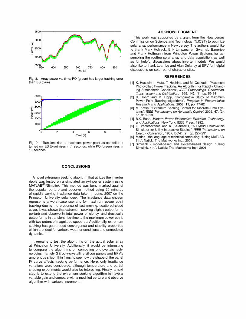
Fig. 8. Array power vs. time; PO (green) has larger tracking errorthan ES (blue).

Fig. 9. Transient rise to maximum power point as controller isturned on. ES (blue) rises in .1 seconds, while PO (green) rises in10 seconds.

CONCLUSIONS

A novel extremum seeking algorithm that utilizes the inverterripple was tested on a simulated array-inverter system usingMATLAB R©/Simulink. This method was benchmarked againstthe popular perturb and observe method using 25 minutesof rapidly varying irradiance data taken in June, 2007 on thePrinceton University solar deck. The irradiance data chosenrepresents a worst-case scenario for maximum power pointtracking due to the presence of fast moving, scattered cloudcover. It was shown that extremum seeking slightly outperformsperturb and observe in total power efficiency, and drasticallyoutperforms in transient rise-time to the maximum power point,with two orders of magnitude speed-up. Additionally, extremumseeking has guaranteed convergence and stability propertieswhich are ideal for variable weather conditions and unmodeleddynamics.

It remains to test the algorithms on the actual solar arrayat Princeton University. Additionally, it would be interestingto compare the algorithms on competing photovoltaic tech-nologies, namely GE poly-crystalline silicon panels and EPV’samorphous silicon thin films, to see how the shape of the panelIV curve affects tracking performance. Here, only irradiancevariations were considered, although temperature and partialshading experiments would also be interesting. Finally, a nextstep is to extend the extremum seeking algorithm to have avariable gain and compare with a modified perturb and observealgorithm with variable increment.

ACKNOWLEDGMENTThis work was supported by a grant from the New Jersey

Commission on Science and Technology (NJCST) to optimizesolar array performance in New Jersey. The authors would liketo thank Mark Holveck, Erik Limpaecher, Swarnab Banerjeeand Frank Hoffmann from Princeton Power Systems for as-sembling the rooftop solar array and data acquisition, as wellas for helpful discussions about inverter models. We wouldalso like to thank Loan Le and Alan Delahoy at EPV for helpfuldiscussions on solar panel characteristics.

REFERENCES

[1] K. Hussein, I. Muta, T. Hoshino, and M. Osakada, ”MaximumPhotovoltaic Power Tracking: An Algorithm for Rapidly Chang-ing Atmospheric Conditions”, IEEE Proceedings. Generation,Transmission and Distribution, 1995, 142, (1), pp. 59-64

[2] D. Hohm and M. Ropp, ”Comparative Study of MaximumPower Point Tracking Algorithms”, Progress in Photovoltaics:Research and Applications, 2003, 11, pp. 47-62

[3] M. Krstic, ”Extremum Seeking Control for Discrete-Time Sys-tems”, IEEE Transactions on Automatic Control, 2002, 47, (2),pp. 318-323

[4] B.K. Bose, Modern Power Electronics: Evolution, Technology,and Applications. New York: IEEE Press, 1992.

[5] G. Vachtsevanos and K. Kalaitzakis, ”A Hybrid PhotovoltaicSimulator for Utility Interactive Studies”, IEEE Transactions onEnergy Conversion, 1987, EC-2, (2), pp. 227-231

[6] Matlab - the language of technical computing. ”Using MATLAB,6th.”, Natick: The Mathworks Inc.; 2001.

[7] Simulink - model-based and system-based design. ”UsingSimulink, 4th.”, Natick: The Mathworks Inc.; 2001.