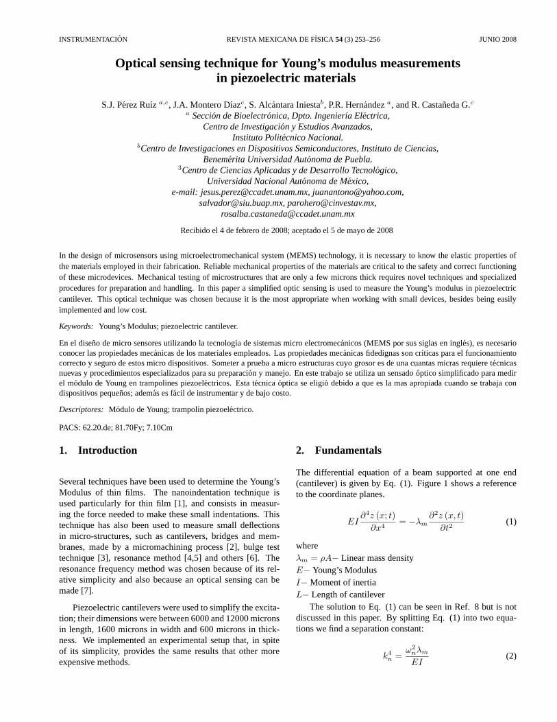
INSTRUMENTACION REVISTA MEXICANA DE FISICA 54 (3) 253–256 JUNIO 2008
Optical sensing technique for Young’s modulus measurementsin piezoelectric materials
S.J. Perez Ruız a,c, J.A. Montero Dıazc, S. Alcantara Iniestab, P.R. Hernandeza, and R. Castaneda G.ca Seccion de Bioelectronica, Dpto. Ingenierıa Electrica,
Centro de Investigacion y Estudios Avanzados,Instituto Politecnico Nacional.
bCentro de Investigaciones en Dispositivos Semiconductores, Instituto de Ciencias,Benemerita Universidad Autonoma de Puebla.
3Centro de Ciencias Aplicadas y de Desarrollo Tecnologico,Universidad Nacional Autonoma de Mexico,
e-mail: [email protected], [email protected],[email protected], [email protected],
Recibido el 4 de febrero de 2008; aceptado el 5 de mayo de 2008
In the design of microsensors using microelectromechanical system (MEMS) technology, it is necessary to know the elastic properties ofthe materials employed in their fabrication. Reliable mechanical properties of the materials are critical to the safety and correct functioningof these microdevices. Mechanical testing of microstructures that are only a few microns thick requires novel techniques and specializedprocedures for preparation and handling. In this paper a simplified optic sensing is used to measure the Young’s modulus in piezoelectriccantilever. This optical technique was chosen because it is the most appropriate when working with small devices, besides being easilyimplemented and low cost.
Keywords: Young’s Modulus; piezoelectric cantilever.
En el diseno de micro sensores utilizando la tecnologıa de sistemas micro electromecanicos (MEMS por sus siglas en ingles), es necesarioconocer las propiedades mecanicas de los materiales empleados. Las propiedades mecanicas fidedignas son crıticas para el funcionamientocorrecto y seguro de estos micro dispositivos. Someter a prueba a micro estructuras cuyo grosor es de una cuantas micras requiere tecnicasnuevas y procedimientos especializados para su preparacion y manejo. En este trabajo se utiliza un sensadooptico simplificado para medirel modulo de Young en trampolines piezoelectricos. Esta tecnicaoptica se eligio debido a que es la mas apropiada cuando se trabaja condispositivos pequenos; ademas es facil de instrumentar y de bajo costo.
Descriptores: Modulo de Young; trampolın piezoelectrico.
PACS: 62.20.de; 81.70Fy; 7.10Cm
1. Introduction
Several techniques have been used to determine the Young’sModulus of thin films. The nanoindentation technique isused particularly for thin film [1], and consists in measur-ing the force needed to make these small indentations. Thistechnique has also been used to measure small deflectionsin micro-structures, such as cantilevers, bridges and mem-branes, made by a micromachining process [2], bulge testtechnique [3], resonance method [4,5] and others [6]. Theresonance frequency method was chosen because of its rel-ative simplicity and also because an optical sensing can bemade [7].
Piezoelectric cantilevers were used to simplify the excita-tion; their dimensions were between 6000 and 12000 micronsin length, 1600 microns in width and 600 microns in thick-ness. We implemented an experimental setup that, in spiteof its simplicity, provides the same results that other moreexpensive methods.
2. Fundamentals
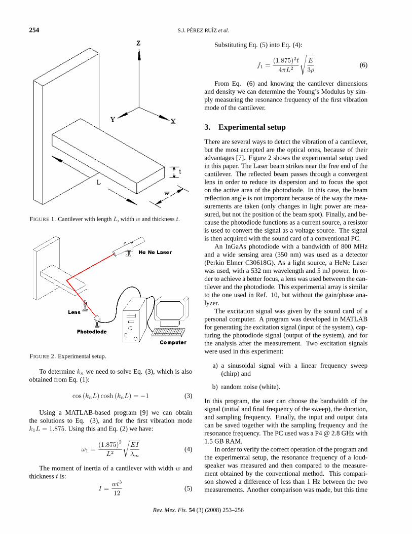
The differential equation of a beam supported at one end(cantilever) is given by Eq. (1). Figure 1 shows a referenceto the coordinate planes.
EI∂4z (x; t)
∂x4= −λm
∂2z (x, t)∂t2
(1)
whereλm = ρA− Linear mass densityE− Young’s ModulusI− Moment of inertiaL− Length of cantilever
The solution to Eq. (1) can be seen in Ref. 8 but is notdiscussed in this paper. By splitting Eq. (1) into two equa-tions we find a separation constant:
k4n =
ω2nλm
EI(2)
254 S.J. PEREZ RUIZ et al.
FIGURE 1. Cantilever with lengthL, width w and thicknesst.
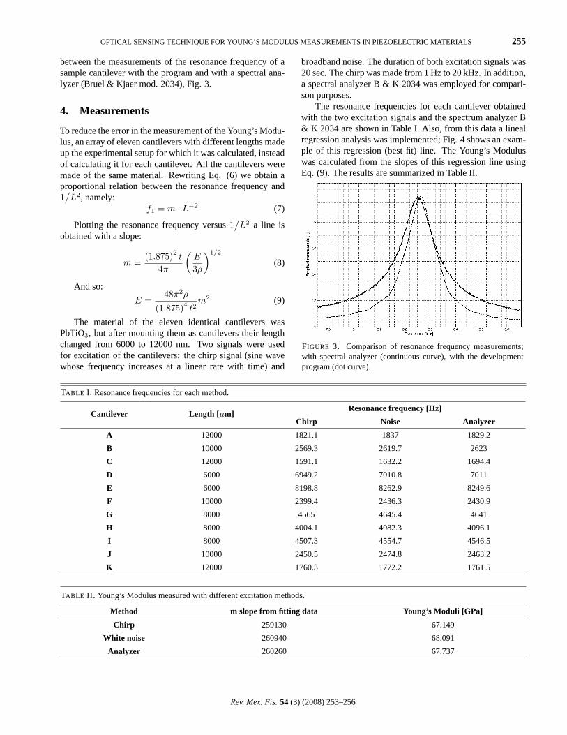
FIGURE 2. Experimental setup.
To determinekn we need to solve Eq. (3), which is alsoobtained from Eq. (1):
cos (knL) cosh (knL) = −1 (3)
Using a MATLAB-based program [9] we can obtainthe solutions to Eq. (3), and for the first vibration modek1L = 1.875. Using this and Eq. (2) we have:
ω1 =(1.875)2
L2
√EI
λm(4)
The moment of inertia of a cantilever with widthw andthicknesst is:
I =wt3
12(5)
Substituting Eq. (5) into Eq. (4):
f1 =(1.875)2t
4πL2
√E
3ρ(6)
From Eq. (6) and knowing the cantilever dimensionsand density we can determine the Young’s Modulus by sim-ply measuring the resonance frequency of the first vibrationmode of the cantilever.
3. Experimental setup
There are several ways to detect the vibration of a cantilever,but the most accepted are the optical ones, because of theiradvantages [7]. Figure 2 shows the experimental setup usedin this paper. The Laser beam strikes near the free end of thecantilever. The reflected beam passes through a convergentlens in order to reduce its dispersion and to focus the spoton the active area of the photodiode. In this case, the beamreflection angle is not important because of the way the mea-surements are taken (only changes in light power are mea-sured, but not the position of the beam spot). Finally, and be-cause the photodiode functions as a current source, a resistoris used to convert the signal as a voltage source. The signalis then acquired with the sound card of a conventional PC.
An InGaAs photodiode with a bandwidth of 800 MHzand a wide sensing area (350 nm) was used as a detector(Perkin Elmer C30618G). As a light source, a HeNe Laserwas used, with a 532 nm wavelength and 5 mJ power. In or-der to achieve a better focus, a lens was used between the can-tilever and the photodiode. This experimental array is similarto the one used in Ref. 10, but without the gain/phase ana-lyzer.
The excitation signal was given by the sound card of apersonal computer. A program was developed in MATLABfor generating the excitation signal (input of the system), cap-turing the photodiode signal (output of the system), and forthe analysis after the measurement. Two excitation signalswere used in this experiment:
a) a sinusoidal signal with a linear frequency sweep(chirp) and
b) random noise (white).
In this program, the user can choose the bandwidth of thesignal (initial and final frequency of the sweep), the duration,and sampling frequency. Finally, the input and output datacan be saved together with the sampling frequency and theresonance frequency. The PC used was a P4 @ 2.8 GHz with1.5 GB RAM.
In order to verify the correct operation of the program andthe experimental setup, the resonance frequency of a loud-speaker was measured and then compared to the measure-ment obtained by the conventional method. This compari-son showed a difference of less than 1 Hz between the twomeasurements. Another comparison was made, but this time
Rev. Mex. Fıs. 54 (3) (2008) 253–256
OPTICAL SENSING TECHNIQUE FOR YOUNG’S MODULUS MEASUREMENTS IN PIEZOELECTRIC MATERIALS 255
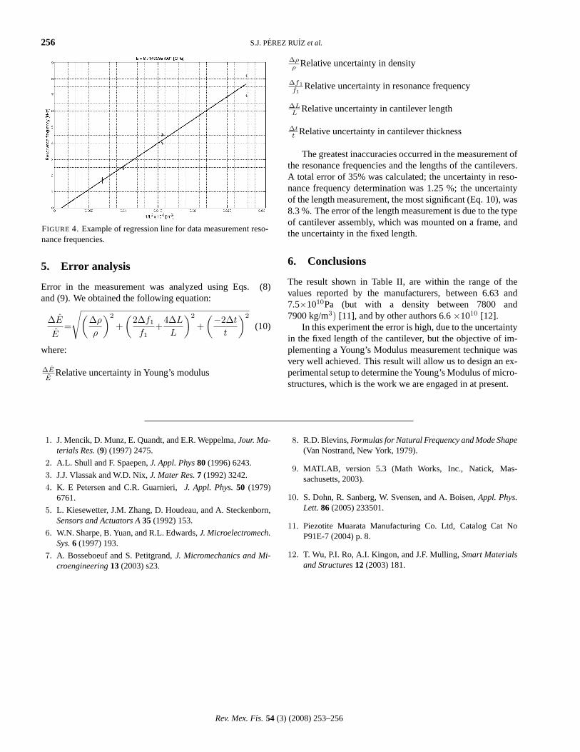
between the measurements of the resonance frequency of asample cantilever with the program and with a spectral ana-lyzer (Bruel & Kjaer mod. 2034), Fig. 3.
4. Measurements
To reduce the error in the measurement of the Young’s Modu-lus, an array of eleven cantilevers with different lengths madeup the experimental setup for which it was calculated, insteadof calculating it for each cantilever. All the cantilevers weremade of the same material. Rewriting Eq. (6) we obtain aproportional relation between the resonance frequency and1/L2, namely:
f1 = m · L−2 (7)
Plotting the resonance frequency versus1/L2 a line is
obtained with a slope:
m =(1.875)2 t
4π
(E
3ρ
)1/2
(8)
And so:
E =48π2ρ
(1.875)4 t2m2 (9)
The material of the eleven identical cantilevers wasPbTiO3, but after mounting them as cantilevers their lengthchanged from 6000 to 12000 nm. Two signals were usedfor excitation of the cantilevers: the chirp signal (sine wavewhose frequency increases at a linear rate with time) and
broadband noise. The duration of both excitation signals was20 sec. The chirp was made from 1 Hz to 20 kHz. In addition,a spectral analyzer B & K 2034 was employed for compari-son purposes.
The resonance frequencies for each cantilever obtainedwith the two excitation signals and the spectrum analyzer B& K 2034 are shown in Table I. Also, from this data a linealregression analysis was implemented; Fig. 4 shows an exam-ple of this regression (best fit) line. The Young’s Moduluswas calculated from the slopes of this regression line usingEq. (9). The results are summarized in Table II.
FIGURE 3. Comparison of resonance frequency measurements;with spectral analyzer (continuous curve), with the developmentprogram (dot curve).
TABLE I. Resonance frequencies for each method.
Cantilever Length [µm]Resonance frequency [Hz]
Chirp Noise Analyzer
A 12000 1821.1 1837 1829.2
B 10000 2569.3 2619.7 2623
C 12000 1591.1 1632.2 1694.4
D 6000 6949.2 7010.8 7011
E 6000 8198.8 8262.9 8249.6
F 10000 2399.4 2436.3 2430.9
G 8000 4565 4645.4 4641
H 8000 4004.1 4082.3 4096.1
I 8000 4507.3 4554.7 4546.5
J 10000 2450.5 2474.8 2463.2
K 12000 1760.3 1772.2 1761.5
TABLE II. Young’s Modulus measured with different excitation methods.
Method m slope from fitting data Young’s Moduli [GPa]
Chirp 259130 67.149
White noise 260940 68.091
Analyzer 260260 67.737
Rev. Mex. Fıs. 54 (3) (2008) 253–256
256 S.J. PEREZ RUIZ et al.
FIGURE 4. Example of regression line for data measurement reso-nance frequencies.
5. Error analysis
Error in the measurement was analyzed using Eqs. (8)and (9). We obtained the following equation:
∆E
E=
√(∆ρ
ρ
)2
+(
2∆f1
f1+
4∆L
L
)2
+(−2∆t
t
)2
(10)
where:
∆EE
Relative uncertainty in Young’s modulus
∆ρρ Relative uncertainty in density
∆f1f1
Relative uncertainty in resonance frequency
∆LL Relative uncertainty in cantilever length
∆tt Relative uncertainty in cantilever thickness
The greatest inaccuracies occurred in the measurement ofthe resonance frequencies and the lengths of the cantilevers.A total error of 35% was calculated; the uncertainty in reso-nance frequency determination was 1.25 %; the uncertaintyof the length measurement, the most significant (Eq. 10), was8.3 %. The error of the length measurement is due to the typeof cantilever assembly, which was mounted on a frame, andthe uncertainty in the fixed length.
6. Conclusions
The result shown in Table II, are within the range of thevalues reported by the manufacturers, between 6.63 and7.5×1010Pa (but with a density between 7800 and7900 kg/m3) [11], and by other authors 6.6×10¹⁰ [12].
In this experiment the error is high, due to the uncertaintyin the fixed length of the cantilever, but the objective of im-plementing a Young’s Modulus measurement technique wasvery well achieved. This result will allow us to design an ex-perimental setup to determine the Young’s Modulus of micro-structures, which is the work we are engaged in at present.
1. J. Mencik, D. Munz, E. Quandt, and E.R. Weppelma,Jour. Ma-terials Res.(9) (1997) 2475.
2. A.L. Shull and F. Spaepen,J. Appl. Phys80 (1996) 6243.
3. J.J. Vlassak and W.D. Nix,J. Mater Res.7 (1992) 3242.
4. K. E Petersen and C.R. Guarnieri,J. Appl. Phys.50 (1979)6761.
5. L. Kiesewetter, J.M. Zhang, D. Houdeau, and A. Steckenborn,Sensors and Actuators A35 (1992) 153.
6. W.N. Sharpe, B. Yuan, and R.L. Edwards,J. Microelectromech.Sys.6 (1997) 193.
7. A. Bosseboeuf and S. Petitgrand,J. Micromechanics and Mi-croengineering13 (2003) s23.
8. R.D. Blevins,Formulas for Natural Frequency and Mode Shape(Van Nostrand, New York, 1979).
9. MATLAB, version 5.3 (Math Works, Inc., Natick, Mas-sachusetts, 2003).
10. S. Dohn, R. Sanberg, W. Svensen, and A. Boisen,Appl. Phys.Lett.86 (2005) 233501.
11. Piezotite Muarata Manufacturing Co. Ltd, Catalog Cat NoP91E-7 (2004) p. 8.
12. T. Wu, P.I. Ro, A.I. Kingon, and J.F. Mulling,Smart Materialsand Structures12 (2003) 181.
Rev. Mex. Fıs. 54 (3) (2008) 253–256
Recommended