Download pdf - Parameterized and approximation algorithms for maximum agreement forest in multifurcating trees

Theoretical Computer Science 562 (2015) 496–512

Contents lists available at ScienceDirect

Theoretical Computer Science

www.elsevier.com/locate/tcs

Parameterized and approximation algorithms for maximum

agreement forest in multifurcating trees

Jianer Chen a,∗, Jia-Hao Fan a, Sing-Hoi Sze a,b

a Department of Computer Science & Engineering, Texas A&M University, College Station, TX 77843, USAb Department of Biochemistry & Biophysics, Texas A&M University, College Station, TX 77843, USA

a r t i c l e i n f o a b s t r a c t

Article history:Received 11 August 2013Received in revised form 1 October 2014Accepted 21 October 2014Available online 27 October 2014Communicated by G. Ausiello

Keywords:Approximation algorithmFixed-parameter tractabilityPhylogenetic treeMaximum agreement forest

We study parameterized algorithms and approximation algorithms for the maximum agreement forest problem, which, for two given leaf-labeled trees, is to find a maximum forest that is a subgraph of both trees. The problem was motivated by research in phylogenetics. For parameterized algorithms, while the problem is known to be fixed-parameter tractable for binary trees, it was an open problem whether the problem is still fixed-parameter tractable for general trees. We resolve this open problem by developing an O (3kn)-time parameterized algorithm for general trees. Our techniques on tree structures also lead to a polynomial-time approximation algorithm of ratio 3 for the problem, giving the first constant-ratio approximation algorithm for general trees.

© 2014 Elsevier B.V. All rights reserved.

1. Introduction

The evolutionary relationships between a set of species are usually represented by a phylogenetic tree in which each leaf is labeled by a distinct species. While a popular way to construct a phylogenetic tree is to start from multiple alignments of genes over a given set of species, different methods often lead to different trees. The use of different sets of aligned genes in the given species can also lead to gene trees that are different from the species tree.

In order to facilitate the comparison of different phylogenetic trees, several distance metrics have been proposed for measuring their similarity [1,8,10,12,13]. A graph theoretical model, the maximum agreement forest (abbr. MAF) has also been proposed that provides a combinatorial structure for the study of the comparison of phylogenetic trees. In particular, the tree-bisection-and-reconnection (TBR) and the subtree-prune-and-regraft (SPR) distances [2,11,20] have direct correspondences to the size of a maximum agreement forest on unrooted trees [1] and on rooted trees [6], respectively.

While most previous work on MAF is restricted to bifurcating (i.e., binary) trees, the problem and related problems on multifurcating (i.e., general) trees have drawn attention recently. Multifurcating phylogenetic trees have appeared quite often in the research of evolutionary biology [3,14,15,19]. Moreover, the relationship between MAF and tree distance metrics on binary trees can be naturally extended to that on multifurcating trees (e.g., see Theorem 2.1 in the next section). The focus of the current paper is on algorithms for the MAF problem on unrooted general trees, which corresponds to the TBR distance on general phylogenetic trees [1].

* Corresponding author.E-mail addresses: [email protected] (J. Chen), [email protected] (J.-H. Fan), [email protected] (S.-H. Sze).

http://dx.doi.org/10.1016/j.tcs.2014.10.0310304-3975/© 2014 Elsevier B.V. All rights reserved.

http://dx.doi.org/10.1016/j.tcs.2014.10.031

http://www.ScienceDirect.com/

http://www.elsevier.com/locate/tcs

mailto:[email protected]



http://dx.doi.org/10.1016/j.tcs.2014.10.031

http://crossmark.crossref.org/dialog/?doi=10.1016/j.tcs.2014.10.031&domain=pdf

J. Chen et al. / Theoretical Computer Science 562 (2015) 496–512 497

Review on related research. The problem of constructing an MAF for two unrooted trees is NP-hard and MAX SNP-hard, even when it is restricted to binary trees [1,5].

Approximation algorithms have been studied for the problem, mainly on binary trees. An approximation algorithm of ratio 3 for the problem on rooted binary trees was claimed by Hein et al. [12], who also claimed that the MAF problem on rooted binary trees corresponds to the SPR distance. Allen and Steel [1] showed that the claim in [12] on the relation-ship between MAF and SPR was not true, and, on the other hand, proved that the MAF problem on unrooted binary trees corresponds to the TBR distance. Rodrigues et al. [17] found a subtle error in [12] and showed that the algorithm in [12]has ratio at least 4. Rodrigues et al. [17] then presented a new approximation algorithm and claimed that their algorithm has ratio 3. Bonet et al. [4] provided a counterexample and showed that for the TBR distance, the algorithm in [12] has approximation ratio at least 5 while the algorithm in [17] has approximation ratio at least 4. Using very different methods, Chataigner [7] developed an approximation algorithm of ratio 8 for the TBR distance for two or more binary trees. Recently, Whidden et al. [20,21] presented a linear-time approximation algorithm of ratio 3 for the TBR distance on unrooted binary trees. This is the best known approximation algorithm for the TBR distance on binary trees. We note that there is also a line of research on another metric, the rSPR distance, on binary trees [4,21], for which the best approximation algorithm has ratio 3 and runs in linear time [20,21]. For general trees, to our knowledge, there are currently no known approximation algorithms for the TBR distance. For the SPR distance on rooted general trees, Rodrigues et al. [18] developed an approxi-mation algorithm of ratio d + 1, where d is the maximum number of children a node in the input trees may have. There is also a line of research on the maximum acyclic agreement forest problem on general trees [16].

Parameterized algorithms for the MAF problem, parameterized by the number k of trees in the MAF, have also been studied. We say that a problem is fixed-parameter tractable [9] if it is solvable in time f (k)nO (1) , where k is the parameter and f (k) is a function independent of the input size n. Allen and Steel [1] showed that the MAF problem on unrooted binary trees, which corresponds to the TBR distance, is fixed-parameter tractable. By branching based on inconsistent structures in quartets, Hallett and McCartin [11] developed an algorithm of time O (4kk5 + nO (1)) for the problem. Whidden and Zeh [21,20] further improved the time complexity to O (4kn), which is currently the best known parameterized algorithm for the MAF problem on unrooted binary trees. For the MAF problem on rooted binary trees, Bordewich et al. [5] proposed a parameterized algorithm of time O (4kk4 + n3), and Whidden et al. [20,21] improved the time complexity to O (2.42kn). While there has been significant work that shows the fixed-parameter tractability for the MAF problem and related problems on binary trees, it was unknown whether the MAF problem on general trees is fixed-parameter tractable or not. This has been posed specifically as an open problem by a number of researchers [11,20].

Our contributions. Our focus is on parameterized algorithms and approximation algorithms for the MAF problem on unrooted general trees. Our method is based on a careful study of the graph structures that takes advantage of spe-cial relationships among sibling leaves in the given trees. We develop an O (3kn)-time parameterized algorithm for the MAF problem on unrooted general trees, thus showing the fixed-parameter tractability of the problem and resolving the open problem posed in [11,20]. In fact, our algorithm is even faster than the previous best parameterized algorithm for the problem on binary trees, which runs in time O (4kn) [21]. We also present a polynomial-time approximation algo-rithm of ratio 3 for the MAF problem on unrooted general trees. The ratio matches the best known approximation ratio for the problem on unrooted binary trees [20,21], but our algorithm keeps the same constant ratio and works for gen-eral trees. The only previously known approximation algorithm for the MAF problem on general trees [18] is on rooted trees and has a ratio of d + 1, where d is the maximum number of children a node in the trees may have. Our algo-rithm is the first constant-ratio approximation algorithm for the MAF problem on general trees, which is on unrooted trees.

2. Preliminaries and problem reformulations

In this paper, all graphs are undirected. For a vertex v , an edge e, and an edge subset E ′ in a graph G , denote by G − v , G −e, and G − E ′ the graphs obtained from G with v , e, and the edges in E ′ removed, respectively. All trees in our discussion are unrooted. A leaf of a tree is a vertex of degree less than 2. A forest is a collection of disjoint trees. A nonempty forest F is leaf-labeled over a label-set L if there is a one-to-one mapping from the leaves of F to the elements of L (with all non-leaf vertices unlabeled). The label for a leaf v is denoted by �(v). More generally, for a subforest F ′ of F , denote by �(F ′) the set of labels for the leaves in F ′ .

Two leaf-labeled forests F1 and F2 over the same label-set L are isomorphic if there is a bijection function f between the vertex sets of F1 and F2 such that any two vertices u and v of F1 are adjacent if and only if f (u) and f (v) are adjacent in F2 and the corresponding leaves have the same label. The forests F1 and F2 are homeomorphic if they become isomorphic after contracting all degree-2 vertices (contracting a degree-2 vertex v is to replace the vertex v and its incident edges with a new edge connecting the two neighbors of v). Note that if a leaf-labeled forest F1 is homeomorphic to a subforest of a leaf-labeled forest F2, then there is a unique subforest of F2 that is homeomorphic to F1. Therefore, in this case, without any confusion, we can simply say that the forest F1 is a subforest of F2. An agreement forest for two leaf-labeled forests F1 and F2 over the same label-set L is a leaf-labeled forest F ′ over the label-set L such that F ′ is a subforest of both F1 and F2. A maximum agreement forest F∗ (abbr. MAF) for F1 and F2 is an agreement forest for F1 and F2 such that the size of (i.e., the number of trees in) F∗ is minimized over all agreement forests for F1 and F2 [11].

498 J. Chen et al. / Theoretical Computer Science 562 (2015) 496–512

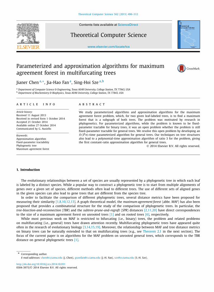
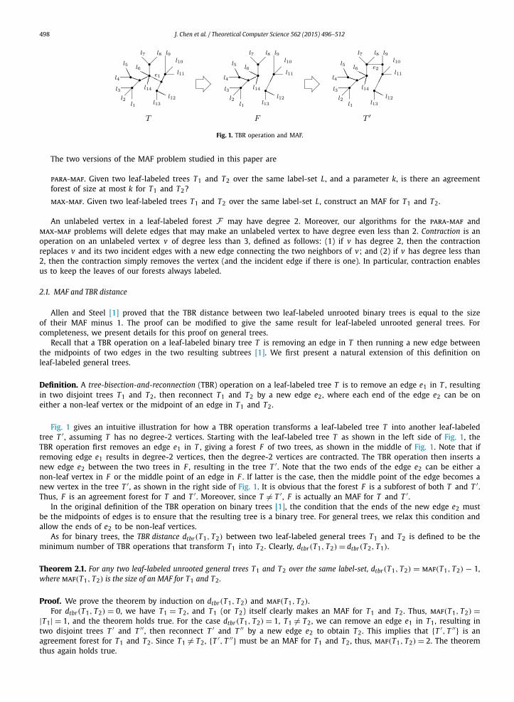
Fig. 1. TBR operation and MAF.

The two versions of the MAF problem studied in this paper are

para-maf. Given two leaf-labeled trees T1 and T2 over the same label-set L, and a parameter k, is there an agreement forest of size at most k for T1 and T2?

max-maf. Given two leaf-labeled trees T1 and T2 over the same label-set L, construct an MAF for T1 and T2.

An unlabeled vertex in a leaf-labeled forest F may have degree 2. Moreover, our algorithms for the para-maf andmax-maf problems will delete edges that may make an unlabeled vertex to have degree even less than 2. Contraction is an operation on an unlabeled vertex v of degree less than 3, defined as follows: (1) if v has degree 2, then the contraction replaces v and its two incident edges with a new edge connecting the two neighbors of v; and (2) if v has degree less than 2, then the contraction simply removes the vertex (and the incident edge if there is one). In particular, contraction enables us to keep the leaves of our forests always labeled.

2.1. MAF and TBR distance

Allen and Steel [1] proved that the TBR distance between two leaf-labeled unrooted binary trees is equal to the size of their MAF minus 1. The proof can be modified to give the same result for leaf-labeled unrooted general trees. For completeness, we present details for this proof on general trees.

Recall that a TBR operation on a leaf-labeled binary tree T is removing an edge in T then running a new edge between the midpoints of two edges in the two resulting subtrees [1]. We first present a natural extension of this definition on leaf-labeled general trees.

Definition. A tree-bisection-and-reconnection (TBR) operation on a leaf-labeled tree T is to remove an edge e1 in T , resulting in two disjoint trees T1 and T2, then reconnect T1 and T2 by a new edge e2, where each end of the edge e2 can be on either a non-leaf vertex or the midpoint of an edge in T1 and T2.

Fig. 1 gives an intuitive illustration for how a TBR operation transforms a leaf-labeled tree T into another leaf-labeled tree T ′ , assuming T has no degree-2 vertices. Starting with the leaf-labeled tree T as shown in the left side of Fig. 1, the TBR operation first removes an edge e1 in T , giving a forest F of two trees, as shown in the middle of Fig. 1. Note that if removing edge e1 results in degree-2 vertices, then the degree-2 vertices are contracted. The TBR operation then inserts a new edge e2 between the two trees in F , resulting in the tree T ′ . Note that the two ends of the edge e2 can be either a non-leaf vertex in F or the middle point of an edge in F . If latter is the case, then the middle point of the edge becomes a new vertex in the tree T ′ , as shown in the right side of Fig. 1. It is obvious that the forest F is a subforest of both T and T ′ . Thus, F is an agreement forest for T and T ′ . Moreover, since T �= T ′ , F is actually an MAF for T and T ′ .

In the original definition of the TBR operation on binary trees [1], the condition that the ends of the new edge e2 must be the midpoints of edges is to ensure that the resulting tree is a binary tree. For general trees, we relax this condition and allow the ends of e2 to be non-leaf vertices.

As for binary trees, the TBR distance dtbr(T1, T2) between two leaf-labeled general trees T1 and T2 is defined to be the minimum number of TBR operations that transform T1 into T2. Clearly, dtbr(T1, T2) = dtbr(T2, T1).

Theorem 2.1. For any two leaf-labeled unrooted general trees T1 and T2 over the same label-set, dtbr(T1, T2) = maf(T1, T2) − 1, where maf(T1, T2) is the size of an MAF for T1 and T2 .

Proof. We prove the theorem by induction on dtbr(T1, T2) and maf(T1, T2).For dtbr(T1, T2) = 0, we have T1 = T2, and T1 (or T2) itself clearly makes an MAF for T1 and T2. Thus, maf(T1, T2) =

|T1| = 1, and the theorem holds true. For the case dtbr(T1, T2) = 1, T1 �= T2, we can remove an edge e1 in T1, resulting in two disjoint trees T ′ and T ′′ , then reconnect T ′ and T ′′ by a new edge e2 to obtain T2. This implies that {T ′, T ′′} is an agreement forest for T1 and T2. Since T1 �= T2, {T ′, T ′′} must be an MAF for T1 and T2, thus, maf(T1, T2) = 2. The theorem thus again holds true.


Now assume dtbr(T1, T2) = d > 1. Then there is a leaf-labeled tree T3 such that dtbr(T1, T3) = d − 1, and dtbr(T3, T2) = 1. By the inductive hypothesis, maf(T1, T3) = d, so T1 and T3 have an MAF F = {T ′

1, · · · , T ′d}, where T ′

i are disjoint subtrees in T3 (and in T1). From dtbr(T3, T2) = 1, the tree T2 can be obtained from the tree T3 by first removing an edge e1then reconnecting the two resulting subtrees by a new edge. This means that T3 \ {e1} is a subforest of T2. Since F is a subforest of T3, F \ {e1} must be a subforest of T2. Therefore, F \ {e1} is an agreement forest for T1 and T2 (note that F is also a subforest of T1). Since F \ {e1} consists of at most d + 1 trees, we get maf(T1, T2) ≤ d + 1, which shows that dtbr(T1, T2) ≥ maf(T1, T2) − 1.

To see the other direction, let maf(T1, T2) = d + 1, where d > 1. Then T1 and T2 have an MAF F = {T ′1, . . . , T

′d+1} with

d + 1 trees. Since T ′1, . . . , T

′d+1 are disjoint in T1, there must be a simple path P1 in T1 that connects two trees in F such

that no internal vertex of P1 is in F . Without loss of generality, suppose that the path P1 has its two end-vertices vdand vd+1 in T ′

d and T ′d+1, respectively. Construct a new tree T3 as follows: First add a new edge e1 between vd and vd+1

in the tree T2, which causes a unique cycle C in T2 ∪ {e1}. Since the edge e1 crosses between two trees in F , there is an edge e2 in the cycle C that is not in F . Now the tree T3 is obtained from T2 ∪ {e1} be removing the edge e2. Note that T ′′

d = T ′d ∪ T ′

d+1 ∪ {e1} is a subtree in both T1 and T3 (for T1, more precisely, T ′′d is homeomorphic to the subtree

T ′d ∪ T ′

d+1 ∪ {P1}). Therefore, {T ′1, . . . , T

′d−1, T

′′d } is an agreement forest for T1 and T3, i.e., maf(T1, T3) ≤ d. By the inductive

hypothesis, dtbr(T1, T3) ≤ d − 1. Because the tree T2 can be obtained from the tree T3 by first removing the edge e1 then adding the edge e2, we conclude immediately

dtbr(T1, T2) ≤ dtbr(T1, T3) + 1 ≤ (d − 1) + 1 = d = maf(T1, T2) − 1.

This completes the proof of the theorem. �2.2. Problem re-formulation

Our algorithms for the MAF problem on a pair (T1, T2) of leaf-labeled trees will proceed by removing edges in the tree T2 to construct a subforest of T2 that is an agreement forest for T1 and T2. Removing edges in T2 will result in a forest consisting of more than one tree. Therefore, our algorithms will really work on two forests F1 and F2. However, the size of an agreement forest F ′ for two forests may not properly reflect the complexity of the construction of F ′: the size of F ′also heavily depends on the sizes of the given forests F1 and F2. Thus, we need a careful reformulation of the problems that allows us to apply a more accurate analysis on the problem complexity.

A partition P = {L1, . . . , Lr} of a label-set L, where Li �= ∅, ⋃r

i=1 Li = L, and Li ∩ L j = ∅, for all i and j, will be called an L-partition, in which each Li is called a label-subset. A label-subset is unit if it consists of a single label. For a leaf-labeled forest F = {T1, . . . , Th} over a label-set L, where each Ti is a leaf-labeled tree, the L-partition {�(T1), . . . , �(Th)} will be called the label-partition for F . For a subset L′ of L, denote by F [L′] the subforest of F induced by L′ , that is, F [L′] consists of all paths in F that connect pairs of leaves with labels in L′ . For an L-partition P = {L1, . . . , Lr} where F [L1], . . . , F [Lr]are vertex-disjoint trees in F , we say that the L-partition P induces the subforest {F [L1], . . . , F [Lr]} of F . An L-partition P is a c-cut label-partition for the forest F , where c ≥ 0 is an integer, if there exists a minimum set Ec of c edges in F such that after removing the c edges in Ec , the label-partition of the resulting forest is P . Note that the label-partition for the forest F is a 0-cut label-partition for F .

Contracting an unlabeled vertex of degree smaller than 2 obviously does not change the label-partition for a forest. For an unlabeled vertex v of degree 2, for which the contraction replaces v and its two incident edges e and e′ with a new edge ev , it is easy to see that the forest obtained by removing any one of e and e′ in the old forest and the forest obtained by removing ev in the new forest have the same label-partition. These observations give immediately the following lemma.

Lemma 2.2. Let F be a leaf-labeled forest over a label-set L, and let F ′ be the forest obtained from F by applying an arbitrary sequence of contractions on F . For any integer c ≥ 0, an L-partition P is a c-cut label-partition for F if and only if P is a c-cut label-partition for F ′ .

The following lemma provides a simple relation between a c-cut label-partition for a leaf-labeled forest F and the number of trees in F .

Lemma 2.3. Suppose that P = {L1, . . . , Lr} is a c-cut label-partition for a leaf-labeled forest F consisting of h trees. Then r = h + c.

Proof. We prove the lemma by induction on c. The lemma obviously holds true for the case c = 0. Consider the case c > 0. Let Ec be a set of c edges in F whose removal results in a forest whose label-partition is P . Let e be any edge in Ec . Then P is a (c − 1)-cut label-partition for the forest F − e. The forest F − e consists of exactly h + 1 trees. By the inductive hypothesis, r = (h + 1) + (c − 1) =h + c. This completes the proof of the lemma. �

Lemma 2.3 directly implies the following corollary, which allows us to characterize agreement forests for two leaf-labeled forests F1 and F2 in terms of c-cut label-partitions for F2.


Corollary 2.4. For an agreement forest F∗ = {T1, . . . , Tk} for two leaf-labeled forests F1 and F2 over the same label-set L, where F2consists of h trees, the L-partition {�(T1), . . . , �(Tk)} is a (k − h)-cut label-partition for F2.

When a c-cut label-partition P for a forest is given, it is easy to find the c edges whose removal results in a forest whose label-partition is P , as shown in the following lemma.

Lemma 2.5. Let L be the label-set for a forest F , and let P = {L1, . . . , Lr} be an L-partition. Let e be an edge in F whose removal splits a leaf-labeled tree in F into two leaf-labeled trees T1 and T2 such that no label-subset in P has labels in both T1 and T2 . Then for any integer c ≥ 1, P is a c-cut label-partition for F if and only if P is a (c − 1)-cut label-partition for F − e.

Proof. Suppose that P is a c-cut label-partition for F . Then F [L1], . . . , F [Lr] are vertex-disjoint trees in F . By the given condition, the edge e is not on a path connecting any two leaves whose labels are in the same label-subset in P . Thus, F [L1], . . . , F [Lr] are still vertex-disjoint trees in the forest F − e, so P is a d-cut label-partition for F − e for some integer d. On the other hand, if P is a d-cut label-partition for F − e, then obviously P is a c-cut label-partition for F for some integer c ≤ d + 1. The equality d = c − 1 follows directly from Lemma 2.3 because the number of trees in F − e is exactly one larger than that in F . �

Corollary 2.4 and Lemma 2.5 suggest a formulation of the MAF problem in terms of c-cut label-partitions. We say that an L-partition P induces an agreement forest for F1 and F2 if the subforest induced by P in F1 and the subforest induced by P in F2 are homeomorphic. By definition, if an L-partition P = {L1, . . . , Lk} induces an agreement forest for F1 and F2, and if F2 consists of h2 trees, then P is a (k − h2)-cut label-partition for F2. This characterization and Lemma 2.5 also provide a convenient way for a branch-and-search process: once we know that an edge e is not on the path connecting any two leaves whose labels are in the same label-subset in the desired (k − h2)-cut label-partition P for the forest F2, we can simply remove e from F2, and recursively construct a (k − h2 − 1)-cut label-partition in the forest F2 − e.

Our study will be based on the following problem formulations using the above characterization.

para-maf’. Given two leaf-labeled forests F1 and F2 over the same label-set L, and a parameter k, is there a k′-cut label-partition for the forest F2 that induces an agreement forest for F1 and F2, where k′ ≤ k?

max-maf’. Given two leaf-labeled forests F1 and F2 over the same label-set L, construct an L-partition P such that Pis a k-cut label-partition for the forest F2 and that P induces an agreement forest for F1 and F2, with k minimized.

An L-partition P will be called a solution for the pair (F1, F2) of leaf-labeled forests over the label-set L if P induces an agreement forest for F1 and F2. The value of the solution P is c if P is a c-cut label-partition for F2. By this definition, constructing a solution of value c for (F1, F2) is to find c edges in F2 whose removal results in a subforest that is an agreement forest for (F1, F2). In particular, by Lemma 2.3, a minimum-value solution for (F1, F2) induces an MAF for F1and F2.

3. Bottommost sibling sets and reduction rules

Because of Lemma 2.2, we will assume that there are no unlabeled vertices of degree less than 3 in a leaf-labeled forest. Moreover, if our algorithms create unlabeled vertices of degree less than 3 during their processing, then we will immediately contract these vertices and work on the resulting forests without unlabeled vertices of degree less than 3.

A tree is a single-vertex tree if it consists of a single vertex, which is a leaf of the tree. A tree is a single-edge tree if it consists of a single edge, which contains two leaves and no non-leaf vertices. The parent of a leaf v in a tree with at least three vertices is the unique non-leaf vertex adjacent to v .

Two leaves in a forest are siblings if they either share the same parent, or are the two leaves of a single-edge tree. A sibling set is a set of leaves that are all siblings. A bottommost sibling set (abbr. BSS) is a maximal sibling set X such that either the degree of their parent is at most |X | + 1, or X is the leaf set of a single-edge tree. By definition, the leaf of a single-vertex tree is not a BSS. Moreover, by our assumption, an unlabeled vertex has degree at least 3. Thus, a BSS contains at least two leaves, and a leaf-labeled tree that is not single-vertex must contain a BSS.

For an illustration, consider the leaf-labeled forest F in Fig. 1. Each of the groups {l1, l2, l3}, {l4, l5}, {l7, l8}, {l9, l10, l11}, and {l12, l13} makes a BSS. On the other hand, l6 and l14 are siblings but do not make a BSS.

In the rest of this section, we fix two leaf-labeled forests F1 and F2 over the same label-set L, and consider their agreement forests. Note that if contraction is not applicable on an agreement forest F∗ for F1 and F2, then each vertex in F∗ corresponds to a unique vertex in F1 as well as to a unique vertex in F2. Therefore, in this case, it makes sense to say that two vertices in F∗ are “adjacent in F1,” or that a vertex v in F∗ is “the parent of a leaf w in F2.” Moreover, because of the one-to-one mapping between the leaf set and the label-set of a leaf-labeled forest, we can conveniently refer to a leaf by its label, without any confusions. For example, we may say that “a label � is in the tree T in the forest F ,” or that “the parent of the label � is the vertex v .”


If F1 consists of only single-vertex trees, then F1 itself is the only agreement forest for F1 and F2. Therefore, in the following discussion, we assume that F1 contains at least one tree that is not a single-vertex tree. Thus, F1 always contains a BSS.

Lemma 3.1. Let X1 be a BSS in F1 , and let P be a solution for the pair (F1, F2). Then P has at most one label-subset Li that intersects �(X1) and |Li | > 1.

Proof. Let F∗ be the agreement forest for F1 and F2 that is induced by P . Let x ∈ X1 such that �(x) ∈ Li and |Li | > 1 for a label-subset Li in P . If X1 is the leaf set of a single-edge tree in F1, then we must have �(X1) = Li and the lemma is proved. If X1 is not the leaf set of a single-edge tree in F1, then since |Li | > 1, the subset F1[Li] must contain the parent of x in F1. Thus, the only way to make a sibling x′ ∈ X1 of x in F1 to be in a disjoint subtree F1[L j], where j �= i, is to cut the edge between x′ and its parent, i.e., L j = {�(x′)} and |L j | = 1. �

Let P be an L-partition, and let Y be a set of leaves in F2. Denote by PY the L-partition that consists of all label-subsets in P that do not intersect �(Y ), plus a label-subset that is the union of all label-subsets in P that intersect �(Y ).

Lemma 3.2. Let X1 be a BSS in the forest F1, and let Y be a sibling set in the forest F2 with �(Y ) ⊆ �(X1). Let P be a solution for the pair (F1, F2) such that a label-subset in P contains at least two labels in �(Y ). Then, the L-partition PY is also a solution for the pair (F1, F2).

Proof. If |Y | ≤ 2, then P = PY and the lemma is obvious. Thus, we can assume that neither X1 nor Y is the leaf set of a single-edge tree. Suppose that the agreement forest for F1 and F2 induced by P = {L1, . . . , Lk} is F∗ = {T1, . . . , Tk}, where �(Ti) = Li for all i, and the tree T1 contains two labels �0 and �1 in �(Y ). Then the parent of �0 and �1 in F1 is in the subtree F1[L1], and the parent of �0 and �1 in F2 is in the subtree F2[L1]. By Lemma 3.1, any other tree in F∗ , say T2, that contains labels in �(Y ) must be a single-vertex tree whose unique label �2 is in �(Y ). Thus, the label subset L1 ∪ L2 = L1 ∪ {�2} induces a subtree T1+2, in both F1 and F2, which is the tree T1 plus a new leaf labeled �2 attached to the parent of �0 and �1. The tree T1+2 intersects no other trees F1[Li] and F2[L j] in F1 and F2, for i, j �= 1, 2. Therefore, the L-partition P ′ = {L1 ∪ L2, L3, . . . , Lk} induces an agreement forest for F1 and F2. Repeating this process shows that the L-partition PY induces an agreement forest for F1 and F2. �

The following lemma shows that a solution for the pair (F1, F2) is symmetric with respect to two labels when certain conditions are enforced.

Lemma 3.3. Let X1 be a BSS in F1 , and let Y be a sibling set in F2 with �(Y ) ⊆ �(X1). For any solution P for (F1, F2), swapping two labels of �(Y ) in P also results in a solution for (F1, F2).

Proof. Let F∗ be the agreement forest for F1 and F2 induced by P . Let y and y′ be in Y whose labels are in different label-subsets in P . By Lemma 3.1, at least one of �(y) and �(y′), say �(y), is in a single-vertex tree Ti in F∗ , where the tree Ti is obtained from F1 and F2 by removing the edge incident to �(y). Since the labels �(y) and �(y′) are symmetric in the forests F1 and F2 (�(y) and �(y′) are siblings in both F1 and F2), removing the edge incident to �(y) and removing the edge incident to �(y′) in F1 or in F2 result in exactly the same forest structure, with only the labels �(y) and �(y′)swapped. Therefore, if the L-partition P induces the agreement forest F∗ for F1 and F2, then by swapping �(y) and �(y′)in P , which corresponds to replacing the removal of the edge incident to �(y) with the removal of the edge incident to �(y′), we get an L-partition that still induces an agreement forest for F1 and F2. �

Now we are able to state our main result in this section, which will play an important role in our algorithms for the maximum agreement forest problems.

Theorem 3.4. Let X1 be a BSS in F1 and let Y be a sibling set in F2 with �(Y ) ⊆ �(X1). For any u0 ∈ Y , there is a maximum agreement forest F∗ for F1 and F2 such that either (1) all labels in �(Y ) are in a single tree in F∗, or (2) each label �(u) in �(Y ), where u �= u0 , is in a single-vertex tree in F∗.

Proof. Let P be the label-partition for a maximum agreement forest F ′ for F1 and F2. If a tree in F ′ contains more than one label in �(Y ), then by Lemma 3.2, the L-partition PY also induces an agreement forest for F1 and F2, where PY is the L-partition that consists of all label-subsets in P that do not intersect �(Y ), plus a label-subset that is the union of all label-subsets in P that intersect �(Y ). The agreement forest induced by PY is obviously maximum and satisfies the condition (1) in the theorem.

If each tree in F ′ contains at most one label in �(Y ), then by Lemma 3.1, at least |Y | − 1 labels in �(Y ) are contained in unit label-subsets in P . If a leaf u �= u0 in Y has its label �(u) in a label-subset in P that is not a unit label-subset, then we


simply swap the labels �(u) and �(u0) in P . By Lemma 3.3, the resulting L-partition P ′ also induces an agreement forest F∗ for F1 and F2, which is obviously also maximum, and satisfies the condition (2) in the theorem. �

In the following, we present two reduction rules on a given pair (F1, F2) of leaf-labeled forests over the same label-set L. The first reduction rule has been observed and used by many other researchers (see, e.g., [1]).

Reduction Rule 1. If a label � is in a single-vertex tree in one of the forests F1 and F2, then remove the edge (if any) incident to the label � in the other forest.

Lemma 3.5. Let (F ′1, F ′

2) be the pair produced by Reduction Rule 1 on the pair (F1, F2), then an L-partition P is a solution of value cfor (F1, F2) if and only if P is a solution of value c′ for (F ′

1, F ′2), where c′ = c − 1 if an edge in F2 is removed, and c′ = c otherwise.

Proof. That the pairs (F1, F2) and (F ′1, F ′

2) have the same collection of solutions follows directly from the fact that if the label � is in a single-vertex tree in one of the forests F1 and F2, then the label � must be in a single-vertex tree in everyagreement forest for F1 and F2. The relation between the values c and c′ follows from Lemma 2.5. �

Let X be a sibling set in a forest. By shrinking X , we mean we delete all leaves in X , and introduce a new leaf v X with a new label �X (e.g., we can use �(X) for �X ), and let v X be adjacent to the common neighbor of the leaves in X if such a common neighbor exists.

Note that if the sibling set X is the leaf set of a single-edge tree, then shrinking X gives a single-vertex tree with the vertex v X . If X is the set of all leaves of a tree with a single non-leaf (and unlabeled) vertex v , then shrinking X makes va degree-1 vertex adjacent to the new leaf v X , and v will be contracted so that the resulting tree becomes a single-vertex tree with the leaf v X .

Reduction Rule 2. Let X1 be a BSS in F1, and let X2 be a set of leaves in F2 such that �(X1) = �(X2). If X2 is the leaf set of a single-edge tree in F2, or if X2 is a sibling set whose parent has degree at most |X2| + 1, then shrink X1 in F1, and shrink X2 in F2.

Note that after applying Reduction Rule 2, if a vertex v in either F1 or F2 is adjacent to the new leaf (there is at most one such vertex), then the degree of v is at most 2. In particular, if v is unlabeled, then v will be contracted.

Lemma 3.6. Let (F ′1, F ′

2) be the pair produced by Reduction Rule 2 on the pair (F1, F2), then the pair (F1, F2) has a solution of value at most c if and only if the pair (F ′

1, F ′2) has a solution of value at most c.

Proof. Suppose that the pair (F ′1, F ′

2) is obtained from the pair (F1, F2) by shrinking a BSS X1 in F1 and the corresponding leaf set X2 in F2 into a single leaf labeled �X2 (= �X1 ).

If the pair (F ′1, F ′

2) has a solution P ′ = {L′1, L

′2, . . . , L

′r} of value c, in which the label �X2 is in the label-subset L′

1, then P = {L1, L2, . . . , Lr} is a solution of value c for the pair (F1, F2), where Li = L′

i for i �= 1, and L1 = (L′1 \ {�X2}) ∪ �(X2).

For the other direction, suppose that the pair (F1, F2) has a solution of value c. Let P = {L1, L2, . . . , Lr} be a solution of minimum value c′ for (F1, F2), where c′ ≤ c and P induces a maximum agreement forest F∗ for F1 and F2. By Theorem 3.4, we can assume that either (1) all labels in �(X2) are in the same tree in F∗ , or (2) each tree in F∗ contains at most one label in �(X2) and at most one tree T0 in F∗ containing a label �0 in �(X2) is not a single-vertex tree. However, case (2) cannot happen: since |X2| ≥ 2, by adding all labels except �0 in �(X2) to the tree T0, we would get an agreement forest for F1 and F2 that consists of fewer trees than F∗ does (note that this can always be done, no matter if the tree T0is a single-vertex tree or not), contradicting the assumption that F∗ is a maximum agreement forest for F1 and F2.

Thus, all labels in �(X2) are in the same tree T in F∗ . Moreover, by the conditions enforced on the sets X1 and X2, all leaves in T with labels in �(X2) are siblings, and if they have a common neighbor v , then v has degree at most |X2| + 1. With all these observations, we derive that if we shrink the leaves with labels in �(X2) in F∗ , we will get a forest F∗∗that is an agreement forest for F ′

1 and F ′2, and the label-partition P ′′ of F∗∗ is a solution of value c′ ≤ c for the pair

(F ′1, F ′

2). �The following theorem follows directly from the definitions of Reduction Rules 1–2.

Theorem 3.7. For a pair (F1, F2) of leaf-labeled forests on which Reduction Rules 1–2 are not applicable, (1) a label is in a single-vertex tree in F1 if and only if it is in a single-vertex tree in F2; and (2) for any sibling set X2 in F2 such that the set X1 in F1 with �(X1) = �(X2) is a BSS, the siblings in X2 must have a parent and the parent has degree at least |X2| + 2.


4. MAF is fixed-parameter tractable

In this section, we present a parameterized algorithm for the para-maf’ problem, and show that the problem, as well as the original para-maf problem, are fixed-parameter tractable.

Let (F1, F2; k) be an instance of the para-maf’ problem, for which we look for a solution of value at most k for the pair (F1, F2) of leaf-labeled forests. Because of Lemmas 3.5 and 3.6, during our process, we will exhaustively apply Reduc-tion Rules 1–2 on the pair of forests whenever the rules are applicable, and work on the reduced instance (note that by Lemma 3.5, in case we apply Reduction Rule 1 that removes an edge in the forest F2, we will also decrease the parameter k by 1). An instance is strongly reduced if none of the contraction operation and Reduction Rules 1–2 are applicable on the corresponding pair of forests. Therefore, throughout the discussion, we will assume that our instance (F1, F2; k) is always a strongly reduced instance.

If all trees in F1 are single-vertex, then by Theorem 3.7, all trees in F2 are also single-vertex, and the problem becomes trivial: F1 =F2 is the unique agreement forest for F1 and F2.

Thus, we can assume that F1 contains a tree that is not single-vertex. As a consequence, there is a BSS X1 in F1 such that |X1| ≥ 2. Let X2 be the leaf set in F2 such that �(X2) = �(X1).

Our algorithm is based on a branch-and-search process. We will introduce a set of branching rules. A branching rule is safe if the branching rule applied on an instance I for para-maf’ produces a set S of instances for para-maf’ such that Iis a yes-instance if and only if at least one of the instances in S is a yes-instance. We say that a branching rule satisfies the recurrence relation T (k) = T (k1) + · · · + T (kr) if on an instance (F1, F2; k) of para-maf’, the branching rule produces rinstances (F1,1, F1,2; k1), . . . , (Fr,1, Fr,2; kr) for the problem. Moreover, we assume that the function T (k) is non-decreasing. Therefore, if k ≤ k′ then T (k) ≤ T (k′).

Case 1. Leaves in X2 are not in the same tree in F2.

Branching Rule 1. Let u2 and v2 be two leaves in X2 that are in different trees in F2, then decrease k by 1, and branch into two ways: [W 1] cut u2 in F2; and [W 2] cut v2 in F2.

Lemma 4.1. Branching Rule 1 is safe, and satisfies the recurrence relation T (k) = 2T (k − 1).

Proof. That the branching rule satisfies the recurrence relation T (k) = 2T (k − 1) follows directly from the rule. Let u1 and v1 be two leaves in F1 such that �(u1) = �(u2) and �(v1) = �(v2). Since u2 and v2 are in different trees in F2, the two labels �(u2) and �(v2) must be in different trees in an agreement forest for F1 and F2. Therefore, in order to construct an agreement forest from F1 for F1 and F2, we must remove edges in F1 to separate the leaves u1 and v1 into two different trees. Because u1 and v1 are siblings, the only way to separate the leaves u1 and v1 into two different trees is to either remove the edge incident to u1 or remove the edge incident to v1. Each of these edge removals makes one of u1 and v1in a single-vertex tree. Therefore, in an agreement forest for F1 and F2, either u2 or v2 must be in a single-vertex tree. As a consequence, at least one of the branching ways [W 1] and [W 2] in the branching rule must correctly remove an edge. Moreover, by Lemma 2.5, a k′-cut label-partition for F2 that induces an agreement forest for F1 and F2, where k′ ≤ k, will become a (k′ − 1)-cut label-partition for the forest obtained from F2 by the correct branch of the branching rule. �Case 2. X2 is a sibling set in F2.

Because the instance (F1, F2; k) is strongly reduced, by Theorem 3.7, X2 has a parent p2 and the degree of p2 is at least |X2| + 2.

Branching Rule 2. If X2 is a sibling set, fix a leaf u2 in X2, and let E2 = {e1, . . . , eh}, h ≥ 2, be the set of edges that are incident to the parent p2 of X2 but not to any leaf in X2. Then branch into h + 1 ways: [W (0)] remove all edges incident to X2 except the one incident to u2 and decrease k by |X2| − 1; and, for each 1 ≤ i ≤ h, [W (i)] remove all edges in E2 except ei and decrease k by h − 1.

Lemma 4.2. Branching Rule 2 is safe, and satisfies the recurrence relation T (k) = T (k − (|X2| − 1)) + hT (k − (h − 1)).

Proof. Again that Branching Rule 2 satisfies the recurrence relation T (k) = T (k − (|X2| −1)) +hT (k − (h −1)) follows directly from the branching rule.

By Theorem 3.4, we can assume that for a maximum agreement forest F∗ for F1 and F2, either all labels in �(X2) are in the same tree in F∗ , or each leaf in X2 \ {u2} has its label in a single-vertex tree in F∗ . In case each leaf in X2 \ {u2} has its label in a single-vertex tree in F∗ , the branching way [W (0)] correctly removes the edges.

Suppose that all labels in �(X2) are in the same tree in F∗ . Then all labels in �(X2) must be siblings in F∗ . Because the parent p1 of X1 has degree at most |X1| + 1, the parent p∗ of the labels in �(X2) in the forest F∗ has its degree at most |X2| + 1. Therefore, in the forest F2, all edges in E2 except at most one must be removed in order to construct F∗ from F2.


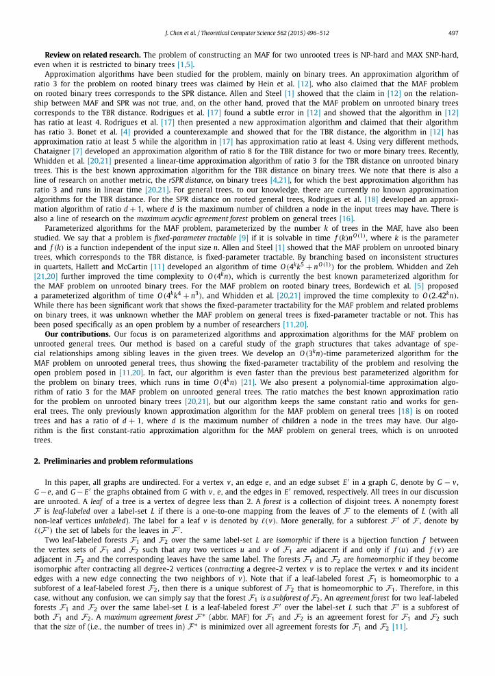
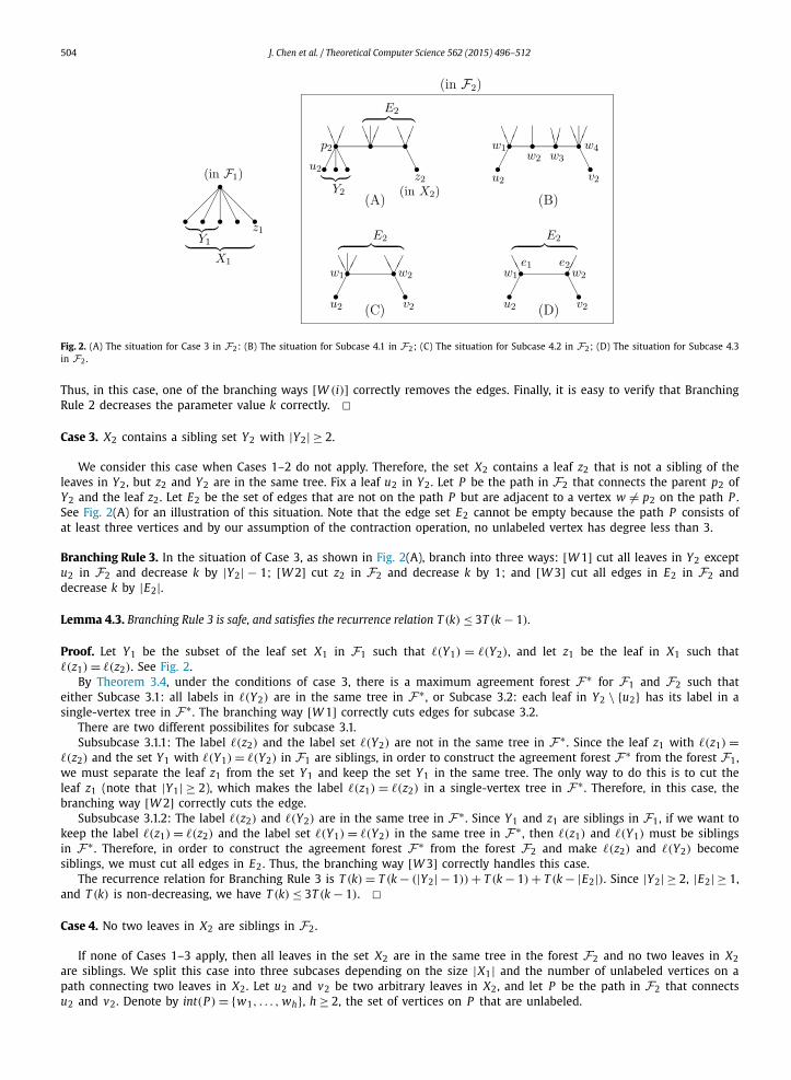
Fig. 2. (A) The situation for Case 3 in F2: (B) The situation for Subcase 4.1 in F2; (C) The situation for Subcase 4.2 in F2; (D) The situation for Subcase 4.3 in F2.

Thus, in this case, one of the branching ways [W (i)] correctly removes the edges. Finally, it is easy to verify that Branching Rule 2 decreases the parameter value k correctly. �Case 3. X2 contains a sibling set Y2 with |Y2| ≥ 2.

We consider this case when Cases 1–2 do not apply. Therefore, the set X2 contains a leaf z2 that is not a sibling of the leaves in Y2, but z2 and Y2 are in the same tree. Fix a leaf u2 in Y2. Let P be the path in F2 that connects the parent p2 of Y2 and the leaf z2. Let E2 be the set of edges that are not on the path P but are adjacent to a vertex w �= p2 on the path P . See Fig. 2(A) for an illustration of this situation. Note that the edge set E2 cannot be empty because the path P consists of at least three vertices and by our assumption of the contraction operation, no unlabeled vertex has degree less than 3.

Branching Rule 3. In the situation of Case 3, as shown in Fig. 2(A), branch into three ways: [W 1] cut all leaves in Y2 except u2 in F2 and decrease k by |Y2| − 1; [W 2] cut z2 in F2 and decrease k by 1; and [W 3] cut all edges in E2 in F2 and decrease k by |E2|.

Lemma 4.3. Branching Rule 3 is safe, and satisfies the recurrence relation T (k) ≤ 3T (k − 1).

Proof. Let Y1 be the subset of the leaf set X1 in F1 such that �(Y1) = �(Y2), and let z1 be the leaf in X1 such that �(z1) = �(z2). See Fig. 2.

By Theorem 3.4, under the conditions of case 3, there is a maximum agreement forest F∗ for F1 and F2 such that either Subcase 3.1: all labels in �(Y2) are in the same tree in F∗ , or Subcase 3.2: each leaf in Y2 \ {u2} has its label in a single-vertex tree in F∗. The branching way [W 1] correctly cuts edges for subcase 3.2.

There are two different possibilites for subcase 3.1.Subsubcase 3.1.1: The label �(z2) and the label set �(Y2) are not in the same tree in F∗ . Since the leaf z1 with �(z1) =

�(z2) and the set Y1 with �(Y1) = �(Y2) in F1 are siblings, in order to construct the agreement forest F∗ from the forest F1, we must separate the leaf z1 from the set Y1 and keep the set Y1 in the same tree. The only way to do this is to cut the leaf z1 (note that |Y1| ≥ 2), which makes the label �(z1) = �(z2) in a single-vertex tree in F∗. Therefore, in this case, the branching way [W 2] correctly cuts the edge.

Subsubcase 3.1.2: The label �(z2) and �(Y2) are in the same tree in F∗ . Since Y1 and z1 are siblings in F1, if we want to keep the label �(z1) = �(z2) and the label set �(Y1) = �(Y2) in the same tree in F∗ , then �(z1) and �(Y1) must be siblings in F∗ . Therefore, in order to construct the agreement forest F∗ from the forest F2 and make �(z2) and �(Y2) become siblings, we must cut all edges in E2. Thus, the branching way [W 3] correctly handles this case.

The recurrence relation for Branching Rule 3 is T (k) = T (k − (|Y2| − 1)) + T (k − 1) + T (k − |E2|). Since |Y2| ≥ 2, |E2| ≥ 1, and T (k) is non-decreasing, we have T (k) ≤ 3T (k − 1). �Case 4. No two leaves in X2 are siblings in F2.

If none of Cases 1–3 apply, then all leaves in the set X2 are in the same tree in the forest F2 and no two leaves in X2are siblings. We split this case into three subcases depending on the size |X1| and the number of unlabeled vertices on a path connecting two leaves in X2. Let u2 and v2 be two arbitrary leaves in X2, and let P be the path in F2 that connects u2 and v2. Denote by int(P ) = {w1, . . . , wh}, h ≥ 2, the set of vertices on P that are unlabeled.


Subcase 4.1: The path P consists of at least five vertices, i.e., h ≥ 3. See Fig. 2(B).

Branching Rule 4.1. Let u2 and v2 be leaves in X2 such that the path P = {u2, w1, . . . , wh, v2} in F2 satisfies h ≥ 3. Then branch into (h + 2) ways: [W 1] cut u2 in F2 and decrease k by 1; [W 2] cut v2 in F2 and decrease k by 1; and, for each 1 ≤ i ≤ h, [W (2 + i)] cut the edges incident to int(P ) \ {wi} but not on the path P , and decrease k by the number of edges cut.

Lemma 4.4. Branching Rule 4.1 is safe, and satisfies the recurrence relation T (k) ≤ 2T (k − 1) + hT (k − (h − 1)).

Proof. Let u1 and v1 be the leaves in the set X1 in the forest F1, with �(u1) = �(u2) and �(v1) = �(v2). Let F∗ be a maximum agreement forest for F1 and F2.

If �(u2) and �(v2) are not in the same tree in F∗ , then to construct F∗ from the forest F1, we need to separate the leaves u1 and v1 in X1 into different trees. Since u1 and v1 are siblings, the only way to separate u1 and v1 is to either cut the edge incident to u1 or cut the edge incident to v1. Each of these makes one of u1 and v1 a single-vertex tree. Thus, in this case, either label �(u2) = �(u1) or label �(v2) = �(v1) is in a single-vertex tree in F∗ . The branching ways [W 1] and [W 2] correctly handle these two cases in F2.

If the labels �(u2) and �(v2) are in the same tree in F∗, then since u1 and v1 are siblings in F1, the labels �(u2) and �(v2) must also be siblings in F∗ . Therefore, in this case, in order to construct the agreement forest F∗ from the forest F2, for all unlabeled vertices w ′ in int(P ), except at most one wi , we must cut all edges incident to w ′ but not on the path P , so that the labels �(u2) and �(v2) can become siblings in F∗ . This case is correctly handled by the branching way [W (2 + i)].

For each i of the branching way [W (2 + i)], we cut hi = ∑j �=i |E ′

j | edges, where E ′j is the set of edges in F2 that are

incident to w j but not on the path P . Thus, the recurrence relation for the branching rule is T (k) = 2T (k −1) +∑i T (k −hi).

Since no unlabeled vertex has degree less than three, |E ′j | ≥ 1 for all j, and hi ≥ h − 1 for all i. Since T (k) is non-decreasing,

we have T (k) ≤ 2T (k − 1) + hT (k − (h − 1)). �Note that if |X2| ≥ 3 and no two leaves in X2 are siblings, then there are always two leaves u2 and v2 in X2 such

that the path connecting u2 and v2 in F2 consists of at least five vertices. In this case, Subcase 4.1 is always applicable. Therefore, in the following, we will assume that the set X2 contains exactly two leaves u2 and v2, the path P connecting u2 and v2 consists of exactly four vertices, of which two are unlabeled, and int(P ) = {w1, w2}. Let E2 be the set of edges that are incident to either w1 or w2 but not on the path P .

Subcase 4.2: E2 = {e1, . . . , eh} with h ≥ 3, see Fig. 2(C).

Branching Rule 4.2. Under the conditions of Subcase 4.2, branch into (2 + h) ways: [W 1] cut u2 in F2 and decrease k by 1; [W 2] cut v2 in F2 and decrease k by 1; and, for each 1 ≤ i ≤ h, [W (2 + i)] for the edge ei in E2, cut all edges in E2 except ei and decrease k by h − 1.

Lemma 4.5. Branching Rule 4.2 is safe, and satisfies the recurrence relation T (k) = 2T (k − 1) + hT (k − (h − 1)).


If the labels �(u2) and �(v2) are not in the same tree in F∗ , then, similar to Subcase 4.1, since u1 and v1 are siblings in F1, at least one of the labels �(u2) and �(v2) must be in a single-vertex tree in F∗ . The branching ways [W 1] and [W 2]correctly handle these cases in F2.

Suppose that �(u2) and �(v2) are in the same tree T in F∗ . If T is a single-edge tree, then all edges in E2 should be removed in F2 to make �(u2) and �(v2) induce a single-edge tree in F∗ . If �(u2) and �(v2) have a parent p∗ in F∗ , then p∗ must correspond to the parent p1 of u1 and v1 in F1. Since u1 and v1 are the only children of p1 and since X1 is a BSS, the vertex p1 has degree at most 3 in F1. As a consequence, the vertex p∗ has degree at most 3 in F∗ . Therefore, all edges in E2 except at most one must be removed when we construct the agreement forest F∗ from F2. These cases are correctly handled by the branching ways [W (2 + i)].

Branching Rule 4.2 satisfies the recurrence relation T (k) = 2T (k − 1) + hT (k − (h − 1)). �Since the leaves u2 and v2 in F2 are not siblings, the path P connecting u2 and v2 has at least two unlabeled vertices.

Since each unlabeled vertex has degree at least three, we must have |E2| ≥ 2. As a consequence, only the case where |E2| = 2 is not covered by the above cases.

Subcase 4.3: E2 = {e1, e2}, see Fig. 2(D).

Branching Rule 4.3. Under the conditions of Subcase 4.3, decrease k by 1, and branch into three ways: [W 0] cut u2 in F2; [W 1] cut e1 in E2; and [W 2] cut e2 in E2.


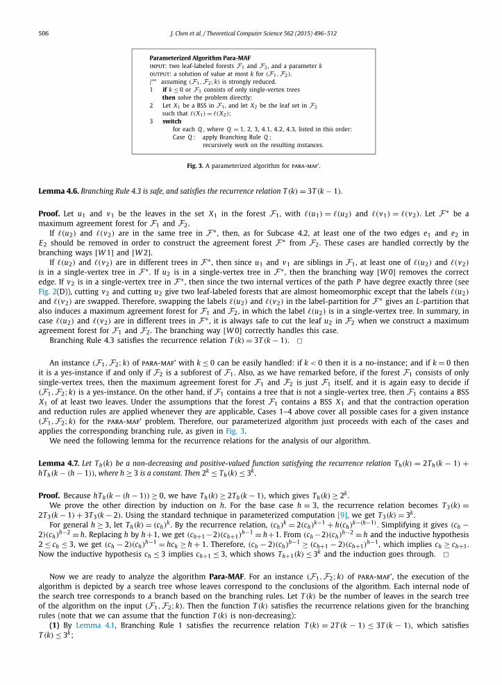
Parameterized Algorithm Para-MAFinput: two leaf-labeled forests F1 and F2, and a parameter koutput: a solution of value at most k for (F1, F2)./** assuming (F1, F2; k) is strongly reduced.1 if k ≤ 0 or F1 consists of only single-vertex trees

then solve the problem directly;2 Let X1 be a BSS in F1, and let X2 be the leaf set in F2

such that �(X1) = �(X2);3 switch

for each Q , where Q = 1, 2, 3, 4.1, 4.2, 4.3, listed in this order:Case Q : apply Branching Rule Q ;

recursively work on the resulting instances.

Fig. 3. A parameterized algorithm for para-maf’.

Lemma 4.6. Branching Rule 4.3 is safe, and satisfies the recurrence relation T (k) = 3T (k − 1).


If �(u2) and �(v2) are in the same tree in F∗ , then, as for Subcase 4.2, at least one of the two edges e1 and e2 in E2 should be removed in order to construct the agreement forest F∗ from F2. These cases are handled correctly by the branching ways [W 1] and [W 2].

If �(u2) and �(v2) are in different trees in F∗ , then since u1 and v1 are siblings in F1, at least one of �(u2) and �(v2)

is in a single-vertex tree in F∗. If u2 is in a single-vertex tree in F∗, then the branching way [W 0] removes the correct edge. If v2 is in a single-vertex tree in F∗ , then since the two internal vertices of the path P have degree exactly three (see Fig. 2(D)), cutting v2 and cutting u2 give two leaf-labeled forests that are almost homeomorphic except that the labels �(u2)

and �(v2) are swapped. Therefore, swapping the labels �(u2) and �(v2) in the label-partition for F∗ gives an L-partition that also induces a maximum agreement forest for F1 and F2, in which the label �(u2) is in a single-vertex tree. In summary, in case �(u2) and �(v2) are in different trees in F∗ , it is always safe to cut the leaf u2 in F2 when we construct a maximum agreement forest for F1 and F2. The branching way [W 0] correctly handles this case.

Branching Rule 4.3 satisfies the recurrence relation T (k) = 3T (k − 1). �An instance (F1, F2; k) of para-maf’ with k ≤ 0 can be easily handled: if k < 0 then it is a no-instance; and if k = 0 then

it is a yes-instance if and only if F2 is a subforest of F1. Also, as we have remarked before, if the forest F1 consists of only single-vertex trees, then the maximum agreement forest for F1 and F2 is just F1 itself, and it is again easy to decide if (F1, F2; k) is a yes-instance. On the other hand, if F1 contains a tree that is not a single-vertex tree, then F1 contains a BSS X1 of at least two leaves. Under the assumptions that the forest F1 contains a BSS X1 and that the contraction operation and reduction rules are applied whenever they are applicable, Cases 1–4 above cover all possible cases for a given instance (F1, F2; k) for the para-maf’ problem. Therefore, our parameterized algorithm just proceeds with each of the cases and applies the corresponding branching rule, as given in Fig. 3.

We need the following lemma for the recurrence relations for the analysis of our algorithm.

Lemma 4.7. Let Th(k) be a non-decreasing and positive-valued function satisfying the recurrence relation Th(k) = 2Th(k − 1) +hTh(k − (h − 1)), where h ≥ 3 is a constant. Then 2k ≤ Th(k) ≤ 3k.

Proof. Because hTh(k − (h − 1)) ≥ 0, we have Th(k) ≥ 2Th(k − 1), which gives Th(k) ≥ 2k .We prove the other direction by induction on h. For the base case h = 3, the recurrence relation becomes T3(k) =

2T3(k − 1) + 3T3(k − 2). Using the standard technique in parameterized computation [9], we get T3(k) = 3k .For general h ≥ 3, let Th(k) = (ch)k . By the recurrence relation, (ch)

k = 2(ch)k−1 + h(ch)k−(h−1) . Simplifying it gives (ch −

2)(ch)h−2 = h. Replacing h by h +1, we get (ch+1 −2)(ch+1)h−1 = h +1. From (ch −2)(ch)h−2 = h and the inductive hypothesis

2 ≤ ch ≤ 3, we get (ch − 2)(ch)h−1 = hch ≥ h + 1. Therefore, (ch − 2)(ch)h−1 ≥ (ch+1 − 2)(ch+1)h−1, which implies ch ≥ ch+1.

Now the inductive hypothesis ch ≤ 3 implies ch+1 ≤ 3, which shows Th+1(k) ≤ 3k and the induction goes through. �Now we are ready to analyze the algorithm Para-MAF. For an instance (F1, F2; k) of para-maf’, the execution of the

algorithm is depicted by a search tree whose leaves correspond to the conclusions of the algorithm. Each internal node of the search tree corresponds to a branch based on the branching rules. Let T (k) be the number of leaves in the search tree of the algorithm on the input (F1, F2; k). Then the function T (k) satisfies the recurrence relations given for the branching rules (note that we can assume that the function T (k) is non-decreasing):

(1) By Lemma 4.1, Branching Rule 1 satisfies the recurrence relation T (k) = 2T (k − 1) ≤ 3T (k − 1), which satisfies T (k) ≤ 3k;


(2) By Lemma 4.2, Branching Rule 2 satisfies the recurrence relation

T (k) = T(k − (|X2| − 1

)) + hT(k − (h − 1)

) ≤ T (k − 1) + hT(k − (h − 1)

),

where |X2| ≥ 2 and h ≥ 2. For h = 2, the recurrence relation becomes T (k) ≤ 3T (k − 1), which satisfies T (k) ≤ 3k . For h ≥ 3, the recurrence relation satisfies:

T (k) ≤ T (k − 1) + hT(k − (h − 1)

) ≤ 2T (k − 1) + hT(k − (h − 1)

).

By Lemma 4.7, the function T (k) also satisfies T (k) ≤ 3k;(3) By Lemma 4.3, Branching Rule 3 satisfies the recurrence relation T (k) ≤ 3T (k − 1), which gives T (k) ≤ 3k;(4.1–4.2) By Lemmas 4.4–4.5, Branching Rules 4.1 and 4.2 satisfy the recurrence relation T (k) ≤ 2T (k −1) +hT (k −(h −1)),

where h ≥ 3. By Lemma 4.7, T (k) satisfies T (k) ≤ 3k;(4.3) By Lemma 4.6, Branching Rule 4.3 satisfies the recurrence relation T (k) ≤ 3T (k − 1), which again gives T (k) ≤ 3k .Thus, each of the branching rules in algorithm Para-MAF satisfies the relation T (k) ≤ 3k , which implies, by induction,

that the search tree of the algorithm has at most 3k leaves. This further implies that the total number of branching nodes in the search tree, i.e., the total number of applications of the branching rules in the algorithm, is bounded by O (3k). Moreover, it is not difficult to verify that each of the branching rules takes time O (n), where n is the number of leaves in the input forests. In conclusion, the total time that the algorithm Para-MAF spends on the branching rules is O (3kn).

With a carefully designed data structure, each of the contraction operation and Reduction Rule 1 takes constant time and decreases the number of vertices by at least 1. Finally, since the total number of vertices in all BSSs in F1 is bounded by O (n), the total running time of a series of applications of Reduction Rule 2 is bounded by O (n). As a consequence, we conclude that along each computational path from the root to a leaf in the search tree of the algorithm, the total running time spent on applications of the contraction operations, Reduction Rule 1, and Reduction Rule 2 is bounded by O (n). This gives our main result in this section:

Theorem 4.8. The parameterized problem para-maf’ can be solved in time O (3kn), so the problem is fixed-parameter tractable.

It is straightforward to see how the original problem para-maf is solved using the algorithm Para-MAF, where two leaf-labeled trees T1 and T2 and a parameter k are given, asking if there is an agreement forest of at most k trees for T1and T2. The problem can be regarded as an instance (T1, T2; k − 1) of the para-maf’ problem where we look for a solution of value at most k − 1 for (T1, T2), i.e., a k′-cut label-partition for the forest (i.e., the tree) T2, where k′ ≤ k − 1, which induces an agreement forest (of k′ + 1 ≤ k trees) for T1 and T2.

Corollary 4.9. The parameterized problem para-maf is solvable in time O (3kn), thus, is fixed-parameter tractable.

Corollary 4.9 resolves an open problem posed in the literature [11,21].As observed by an anonymous referee, by trying successive parameter values k, we can solve the more general max-maf

problem in time O (31n + 32n + · · · + 3hn) = O (3hn), where h is the size of a maximum agreement forest of the two given leaf-labeled trees.

5. A constant-ratio approximation algorithm for MAX-MAF

The analysis in previous sections based on BSS also motivates an approximation algorithm for the max-maf’ problem, which is presented in this section.

Recall that the max-maf’ problem on a pair (F1, F2) of leaf-labeled forests over the same label-set L looks for a solution of minimum value, i.e., an L-partition P that induces an agreement forest for F1 and F2 and is a c-cut label-partition for F2 with the value c minimized. A solution of the minimum value will be called an optimal solution, whose value will be called the optimal value for the instance (F1, F2). Recall that a maximum agreement forest for F1 and F2 is induced by an optimal solution for (F1, F2).

Similarly, we will say that an instance (F1, F2) of max-maf’ is strongly reduced if none of the contraction operation and Reduction Rules 1–2 are applicable on the instance. We will always assume that the instances in our discussion are strongly reduced.

An edge-removal meta-step of an algorithm is a collection of consecutive computational steps in the algorithm that on an instance (F1, F2) of max-maf’ removes a set of edges in F2.

Definition. An edge-removal meta-step M keeps ratio r if on an instance (F1, F2) of max-maf’, M removes a set E M of edges in F2 such that |E M | ≤ r(c − c′), where c and c′ are the optimal values for the instances (F1, F2) and (F1, F2 − E M), respectively.

For example, an application of Reduction Rule 1 that removes an edge e in F2 is an edge-removal meta-step that keeps ratio 1 because |E M | = |{e}| = 1, and by Lemma 3.5, the optimal value for (F1, F2 − e) is one less than that for (F1, F2).


Also note that by definition, a meta-step that neither removes edges in F2 nor change the optimal value for the forest pair (such as an application of Reduction Rule 1 that removes an edge in F1) keeps ratio r for any r ≥ 1.

Before we present our algorithm, we observe the following:

Lemma 5.1. Let (F1, F2) be an instance of max-maf’ and let e2 be any edge in F2. Then the optimal value for (F1, F2 − e2) is at most the optimal value for (F1, F2).

Proof. Let P be an optimal solution of value c for (F1, F2), where P is a c-cut label-partition for F2. Then there is a set E2 of c edges in F2 such that after contraction, F2 − E2 (whose label-partition is P) is an agreement forest for (F1, F2). If e2 ∈ E2, then E ′

2 = E2 \ {e2} is a set of c − 1 edges such that (F2 − e2) − E ′2 is an agreement forest for (F1, F2 − e2).

That is, the optimal value for (F1, F2 − e2) is at most |E ′2| = c − 1. On the other hand, if e2 /∈ E2, then since F2 − E2 is an

agreement forest for (F1, F2), removing the edge e2 in F2 − E2 also results in an agreement forest for (F1, F2). That is, (F2 − e2) − E2 is an agreement forest for (F1, F2 − e2), and the optimal value for (F1, F2 − e2) is then at most |E2| = c. �

In the rest of this section, we fix an instance (F1, F2) of the max-maf’ problem. As we have examined in previous sections, we can assume that the instance is strongly reduced, and that the forest F1 contains at least one BSS X1. Let X2be the leaf set in F2 with �(X2) = �(X1).

As we did in the parameterized algorithm, we consider different cases based on the structure of the leaf set X2 in F2. For each case, we apply a meta-step that removes a set of edges in F2 and we verify that the meta-step keeps a ratio bounded by 3.

Case 1. Leaves in X2 are not in the same tree in F2.

Meta-Step 1. Let u2 and v2 be two leaves in X2 that are in different trees in F2, then remove the edges incident to u2and v2.

Lemma 5.2. Meta-Step 1 keeps ratio 2.

Proof. Let P be an optimal solution of value c for the instance (F1, F2), which is a c-cut label-partition for F2. As examined in Lemma 4.1, one of the labels �(u2) and �(v2) is in a unit label-subset in P . Without loss of generality, suppose �(u2) is such a label, and let eu and ev be the edges incident to u2 and v2 in F2, respectively. By Lemma 2.5, P is a (c − 1)-cut label-partition for F2 − eu . Also, P is a solution for (F1, F2 − eu) because u2 is in a unit label-subset in P . Therefore, the optimal value for (F1, F2 − eu) is at most c − 1. Finally, by Lemma 5.1, the optimal vale c′ for (F1, F2 − {eu, ev}) is at most c − 1. Therefore, Meta-Step 1 removes the edge set E1 = {eu, ev} that satisfies |E1| ≤ 2(c − c′), where c and c′ are the optimal values for (F1, F2) and (F1, F2 − E1), respectively. That is, the meta-step keeps ratio 2. �Case 2. X2 is a sibling set in F2.

Because the instance (F1, F2) is strongly reduced, by Theorem 3.7, X2 has a parent p2 and the degree of p2 is at least |X2| + 2. In the following two cases, let E ′′ be the set of edges that are incident to the parent p2 of X2 but not incident to the leaves in X2. We apply the following meta-steps based on the difference between the sizes of X2 and E ′′ . See Figs. 4(A) and 4(B).

Subcase 2.1: |E ′′| > |X2|.

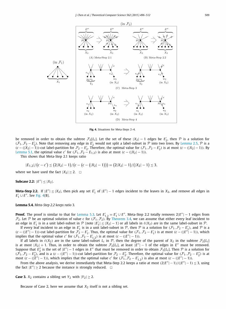
Meta-Step 2.1. If |E ′′| > |X2|, then pick any set E1 of |X2| − 1 edges incident to the leaves in X2, and pick any set E2 of |X2| edges in E ′′ , remove all edges in E1 ∪ E2. See Fig. 4(A).

Lemma 5.3. Meta-Step 2.1 keeps ratio 3.

Proof. Let P be an optimal solution of value c for (F1, F2), which is a c-cut label-partition for F2. Let E1,2 = E1 ∪ E2. Meta-Step 2.1 totally removes |E1,2| = 2|X2| − 1 edges from F2.

By Theorem 3.4, we can assume that either each leaf incident to an edge in E1 is in a unit label-subset in P or all labels in �(X2) are in the same label-subset in P .

If each of the |X2| − 1 leaves incident to the edges in E1 is in a unit label-subset in P , then P is a solution for (F1, F2 − E1). Since removing each edge in E1 does not split a label-subset in P into two trees, by Lemma 2.5, P is a (c − (|X2| − 1))-cut label-partition for F2 − E1. Therefore, the optimal value for (F1, F2 − E1) is at most (c − (|X2| − 1)). By Lemma 5.1, the optimal value c′ for (F1, F2 − E1,2) is also at most (c − (|X2| − 1)).

If all labels in �(X2) are in the same label-subset Li in P , then the degree of the parent of X2 in the subtree F2[Li]is at most |X2| + 1 (because X1 is a BSS). This implies that among the |X2| edges in E2, at least |X2| − 1 of them must


Fig. 4. Situations for Meta-Steps 2–4.

be removed in order to obtain the subtree F2[Li]. Let the set of these |X2| − 1 edges be E ′2, then P is a solution for

(F1, F2 − E ′2). Note that removing any edge in E ′

2 would not split a label-subset in P into two trees. By Lemma 2.5, P is a (c − (|X2| − 1))-cut label-partition for F2 − E ′

2. Therefore, the optimal value for (F1, F2 − E ′2) is at most (c − (|X2| − 1)). By

Lemma 5.1, the optimal value c′ for (F1, F2 − E1,2) is also at most (c − (|X2| − 1)).This shows that Meta-Step 2.1 keeps ratio

|E1,2|/(c − c′) ≤ (

2|X2| − 1)/(c − (

c − (|X2| − 1))) = (

2|X2| − 1)/(|X2| − 1

) ≤ 3,

where we have used the fact |X2| ≥ 2. �Subcase 2.2: |E ′′| ≤ |X2|.

Meta-Step 2.2. If |E ′′| ≤ |X2|, then pick any set E ′1 of |E ′′| − 1 edges incident to the leaves in X2, and remove all edges in

E ′1 ∪ E ′′ . See Fig. 4(B).

Lemma 5.4. Meta-Step 2.2 keeps ratio 3.

Proof. The proof is similar to that for Lemma 5.3. Let E ′1,2 = E ′

1 ∪ E ′′ . Meta-Step 2.2 totally removes 2|E ′′| − 1 edges from F2. Let P be an optimal solution of value c for (F1, F2). By Theorem 3.4, we can assume that either every leaf incident to an edge in E ′

1 is in a unit label-subset in P (note |E ′1| ≤ |X2| − 1) or all labels in �(X2) are in the same label-subset in P .

If every leaf incident to an edge in E ′1 is in a unit label-subset in P , then P is a solution for (F1, F2 − E ′

1), and P is a (c − (|E ′′| − 1))-cut label-partition for F2 − E ′

1. Thus, the optimal value for (F1, F2 − E ′1) is at most (c − (|E ′′| − 1)), which

implies that the optimal value c′ for (F1, F2 − E ′1,2) is at most (c − (|E ′′| − 1)).

If all labels in �(X2) are in the same label-subset Li in P , then the degree of the parent of X2 in the subtree F2[Li]is at most |X2| + 1. Thus, in order to obtain the subtree F2[Li], at least |E ′′| − 1 of the edges in E ′′ must be removed. Suppose that E ′′

2 is the set of |E ′′| − 1 edges in E ′′ that must be removed in order to obtain F2[Li]. Then P is a solution for (F1, F2 − E ′′

2), and is a (c − (|E ′′| − 1))-cut label-partition for F2 − E ′′2. Therefore, the optimal value for (F1, F2 − E ′′

2) is at most (c − (|E ′′| − 1)), which implies that the optimal value c′ for (F1, F2 − E ′

1,2) is also at most (c − (|E ′′| − 1)).From the above analysis, we derive immediately that Meta-Step 2.2 keeps a ratio at most (2|E ′′| −1)/(|E ′′| −1) ≤ 3, using

the fact |E ′′| ≥ 2 because the instance is strongly reduced. �Case 3. X2 contains a sibling set Y2 with |Y2| ≥ 2.

Because of Case 2, here we assume that X2 itself is not a sibling set.


Meta-Step 3. Let u2, v2 ∈ Y2, and let w2 be a leaf in X2 that is not a sibling of u2 and v2. Let e be an edge incident to the parent of w2 but not on the path between u2 and w2. Then remove the edge e, the edge eu incident to u2, and the edge ew incident to w2. See Fig. 4(C).


Proof. Let E3 = {e, eu, ew}. Let P be an optimal solution of value c for (F1, F2). By Theorem 3.4, we can assume that either the label �(u2) is in a unit label-subset in P or both labels �(u2) and �(v2) are in the same label-subset in P .

If �(u2) is in a unit label-subset in P , then P is a solution for (F1, F2 − eu). By Lemma 2.5, P is a (c − 1)-cut label-partition for F2 − eu . This combined with Lemma 5.1 shows that the optimal value for (F1, F2 − E3) is at most c − 1.

Now suppose that �(u2) and �(v2) are in the same label-subset Li in P . If �(w2) is also in Li , then the edge e must be removed because �(u2), �(v2), and �(w2) are siblings in F1. Hence, the optimal value for (F1, F2 − e) (thus the optimal value for (F1, F2 − E3)) is at most c − 1. On the other hand, if �(w2) is not in Li , then �(w2) must be in a unit label-subset in P because the only way to separate �(w2) from the tree containing both �(u2) and �(v2) in the forest F1 is to remove the edge incident to w2. Therefore, in this case, P is a solution for (F1, F2 − ew), and is a (c − 1)-cut label-partition for F2 − ew , which implies again that the optimal value for (F1, F2 − E3) is at most c − 1.

Since Meta-Step 3 totally removes three edges, the above discussion implies directly that the meta-step keeps ratio 3. �When none of the cases 1–3 hold true, all leaves in X2 are in the same tree in F2 but no two are siblings. For this last

case, we first prove the following lemma.

Lemma 5.6. If all leaves in X2 are in the same tree in F2 but no two are siblings, then there is a leaf in X2 whose parent has degree 2in the induced subforest F2[�(X2)].

Proof. The lemma obviously holds true if |X2| = 2 since the two leaves in X2 are not siblings. For |X2| > 2, the tree F2[�(X2)] has at least three unlabeled vertices. Removing all leaves in F2[�(X2)] results in a non-empty tree T ′ . Any leaf in T ′ is a degree-2 vertex in F2[�(X2)] that is a parent of a leaf in X2. �

Case 4. All leaves in X2 are in the same tree in F2 but no two are siblings.

Meta-Step 4. Let u2, v2 ∈ X2 such that the parent p2 of u2 has degree two in F2[�(X2)]. Let e be an edge in F2 that is incident to p2 but not on the path Puv between u2 and v2. Then cut the edge e, the edge eu incident to u2, and the edge ev incident to v2. See Fig. 4(D).


Proof. Let E4 = {e, eu, ev}. Let P be an optimal solution of value c for (F1, F2). If removing any e′ of the edges in E4 does not split any label-subset in P into two trees, then P is a solution for (F1, F2 − e′). By Lemma 2.5, P is a (c − 1)-cut label-partition for F2 − e′ . This combined with Lemma 5.1 shows that the optimal value for (F1, F2 − E4) is at most c − 1.

So we assume that removing any edge in E4 will split some label-subsets in P . In particular, �(u2) and �(v2) are not in unit label-subsets in P . Let F∗ be the maximum agreement forest induced by P . Since �(u2) and �(v2) are siblings in F1, �(u2) and �(v2) must be siblings in F∗ . Since the edge e must remain in F∗ , the vertex p2, which is the parent of u2 in F2, must be the parent of �(u2) and �(v2) in F∗ . By Lemma 5.6, p2 has degree two in F2[�(X2)]. Since p2 corresponds to the parent of �(u2) and �(v2) in F1, which is incident to at most one edge whose other end is not in X1, p2 must have degree exactly three in F∗ (the edge e does not lead to another vertex in X2).

Thus, if we let Euv be the set of all edges, except e, that are incident to a vertex in Puv but not on Puv , then in order to make F∗ from F2, all edges in Euv must be removed. Let Ec be a set of c edges in F2 such that the label-partition for F2 − Ec is P . Since removing any edge in Euv does not split a label-subset in P , we can assume Euv ⊆ Ec . Now removing the edge e in F2 − Ec makes the path Puv become a component of the forest, and removing the edge eu further makes �(u2) and �(v2) become single-vertex trees. Let the resulting forest be F ′ whose label-partition is P ′ . Then both �(u2) and �(v2) are in unit label-subsets in P ′ , and P ′ is a solution for (F1, F2 − E4), as well as a solution for (F1, F2). Moreover, P ′ is a (c + 2)-cut label-partition for F2.

On the other hand, if we cut the edges e, eu , and ev in F2, each cut certainly does not split a label-subset in P ′ . Moreover, since �(u1) and �(v2) are not siblings in F2, cutting each of these edges increases the number of leaf-labeled trees in the forest. Therefore, P ′ is a ((c + 2) − 3)-cut, i.e., a (c − 1)-cut label-partition for F2 − E4. This shows that the optimal value for (F1, F2 − E4) is at most c − 1.

Since |E4| = 3, we conclude that Meta-Step 4 keeps ratio 3. �Now we are ready to present our approximation algorithm, Apx-MAF, for the max-maf’ problem, as given in Fig. 5.


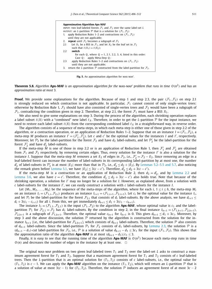
Approximation Algorithm Apx-MAFinput: two leaf-labeled forests F1 and F2 over the same label-set Loutput: an L-partition P that is a solution for (F1, F2)

1. apply Reduction Rules 1–2 and contractions on (F1, F2)

until they are not applicable;2. repeat until F2 becomes a subgraph of F1

2.1 Let X1 be a BSS in F1, and let X2 be the leaf set in F2

such that �(X1) = �(X2);2.2 switch

for each Q , where Q = 1, 2.1, 2.2, 3, 4, listed in this order:Case Q : apply Meta-Step Q ;

2.3 apply Reduction Rules 1–2 and contractions on (F1, F2)

until they are not applicable;3. return the L-partition P constructed from the label-partition for F2.

Fig. 5. An approximation algorithm for max-maf’.

Theorem 5.8. Algorithm Apx-MAF is an approximation algorithm for the max-maf’ problem that runs in time O (n2) and has an approximation ratio at most 3.

Proof. We provide some explanations for the algorithm. Because of step 1 and step 2.3, the pair (F1, F2) on step 2.1 is strongly reduced on which contraction is not applicable. In particular, F1 cannot consist of only single-vertex trees: otherwise by Reduction Rule 1, F2 should have also consisted of single-vertex trees and F2 would have been a subgraph of F1, contradicting the condition given in step 2. Therefore, at step 2.1, the forest F1 must have a BSS X1.

We also need to give some explanations on step 3. During the process of the algorithm, each shrinking operation replaces a label subset �(X) with a “combined” new label �X . Therefore, in order to get the L-partition P for the input instance, we need to restore each label subset �(X) from the corresponding combined label �X in a straightforward way, in reverse order.

The algorithm consists of a sequence of meta-steps, in which each meta-step is either one of those given in step 2.2 of the algorithm, or a contraction operation, or an application of Reduction Rules 1–2. Suppose that on an instance I = (F1, F2), a meta-step M produces an instance I ′ = (F ′

1, F ′2). Let c and c′ be the optimal values for the instances I and I ′ , respectively.

Moreover, let P2 be the label-partition for the forest F2 and have d2 label-subsets, and let P ′2 be the label-partition for the

forest F ′2 and have d′

2 label-subsets.If the meta-step M is one of those in step 2.2 or is an application of Reduction Rule 1, then F ′

1 and F ′2 are obtained

from F1 and F2 respectively, by removing certain edges. Thus, every solution for the instance I ′ is also a solution for the instance I . Suppose that the meta-step M removes a set E2 of edges in F2, i.e., F ′

2 =F2 − E2. Since removing an edge in a leaf-labeled forest can increase the number of label-subsets in its corresponding label-partition by at most one, the number d′

2 of label-subsets in P ′2 is at most |E2| more than that in P2, i.e., d′

2 ≤ d2 + |E2|. By Lemmas 5.2–5.5 and 5.7, also noticing the remark given before Lemma 5.1, we have |E2| ≤ 3(c − c′). Therefore, d′

2 ≤ d2 + 3(c − c′).If the meta-step M is a contraction or an application of Reduction Rule 2, then d2 = d′

2, and by Lemma 2.2 and Lemma 3.6, we also have c = c′ . Therefore, the condition d′

2 ≤ d2 + 3(c − c′) also holds true. Note that because of the shrinking operation, a solution for I ′ may no longer be a solution for I . However, as explained above, from a solution with c label-subsets for the instance I ′ , we can easily construct a solution with c label-subsets for the instance I .

Let {M1, M2, . . . , Mh} be the sequence of the meta-steps of the algorithm, where for each i, 1 ≤ i ≤ h, the meta-step Mion an instance Ii = (F1,i, F2,i) produces an instance Ii+1 = (F1,i+1, F2,i+1). Let ci be the optimal value for the instance Ii , and let Pi be the label-partition for the forest F2,i that consists of di label-subsets. By the above analysis, we have di+1 ≤di + 3(ci − ci+1) for all i. From this, we get immediately dh+1 ≤ d1 + 3(c1 − ch+1).

The instance I1 = (F1,1, F2,1) is the input (F1, F2) to the algorithm Apx-MAF, whose optimal value is c1 and the label-partition P1 for F2,1 = F2 has d1 label-subsets. By the condition in step 2, in the final instance Ih+1 = (F1,h+1, F2,h+1), F2,h+1 is a subgraph of F1,h+1. Therefore, the optimal value ch+1 for Ih+1 is 0. This gives dh+1 ≤ d1 + 3c1. Moreover, by step 3 and the above discussion, the solution P returned by the algorithm is constructed from the solution for the in-stance Ih+1 (i.e., the label-partition for F2,h+1), which consists of dh+1 label-subsets. Therefore, the solution P also consists of dh+1 label-subsets. Since the label-partition P1 for F2 consists of d1 label-subsets, by Lemma 2.3, the solution P is a (dh+1 − d1)-cut label-partition for F2, i.e., P is a solution of value dh+1 − d1 ≤ 3c1 for the input (F1, F2). This shows that the approximation ratio of the algorithm Apx-MAF is at most (dh+1 − d1)/c1 ≤ 3.

Finally, it is easy to see that the running time of the algorithm Apx-MAF is O (n2) because each meta-step runs in time O (n) and decreases the number of edges in the instance by at least one. �

The original max-maf problem on two given leaf-labeled trees T1 and T2 over the label-set L asks to construct a max-imum agreement forest for T1 and T2. Suppose that a maximum agreement forest for T1 and T2 consists of c leaf-labeled trees. Then the L-partition that is an optimal solution for (T1, T2) consists of c label-subsets, i.e., the optimal value for (T1, T2) is c − 1. We can apply the Apx-MAF algorithm on the instance (T1, T2), which will return an L-partition P that is a solution of value at most 3(c − 1) for (T1, T2). Therefore, the solution P induces an agreement forest of at most 3c − 2


trees for (T1, T2). The ratio (3c − 2)/c < 3 shows that Apx-MAF can also be used as an approximation algorithm for the problem max-maf that has an approximation ratio bounded by 3.

When applied on binary trees, the algorithm Apx-MAF with its ratio of 3 matches the best previous known ratio for the problem on binary trees [21]. On the other hand, we note that the algorithm in [21] runs in linear time while the algorithmApx-MAF runs in time O (n2). The only previously known approximation algorithm for the MAF problem on general trees is on rooted trees and has ratio d + 1, where d is the maximum number of children a node in the forests may have [18]. Our algorithm is the first constant-ratio approximation algorithm for the MAF problem on general trees, where the trees are unrooted.

6. Conclusions

As suggested by Whidden, Beiko, and Zeh in their recent publication in SIAM J. Comput. [20], “The most important open problem is extending our approach to computing MAFs and MAAFs for multifurcating trees and for more than two trees.” Our result is a response to this call and makes an important step towards this direction. We have presented a parameterized algorithm and an approximation algorithm for the MAF problem on unrooted general trees, which corresponds to the TBR distance on multifurcating phylogenetic trees. For general trees, our parameterized algorithm is the first fixed-parameter tractable algorithm and our approximation algorithm is the first constant-ratio approximation algorithm. Our algorithms are based on the concept of a bottommost sibling set in one tree and the structure of the corresponding leaf set in the other tree. The methods based on sibling sets have been used by other researchers (e.g., [1,18,20]), but the special structure of the bottommost sibling set enables us to deal with operations on general trees more effectively. The techniques should be useful for the study on parameterized and approximation algorithms for other problems related to phylogenetic similarity, such as those related to the SPR distance and the rooted SPR distance. We are currently working on these extensions and aimed at new and more efficient algorithms for these problems.

Acknowledgements

The authors would like to thank the anonymous referees, whose critical comments and suggestions have been important for improving the presentation of the paper. In particular, a referee provided a very helpful observation that shows how our parameterized algorithm for the para-maf problem is extended to become an optimal algorithm for solving the more general max-maf problem. This observation has been described in the last paragraph in Section 4.

References

[1] B.L. Allen, M. Steel, Subtree transfer operations and their induced metrics on evolutionary trees, Ann. Comb. 5 (1) (2001) 1–15.[2] A. Amir, D. Keselman, Maximum agreement subtree in a set of evolutionary trees: metrics and efficient algorithms, SIAM J. Comput. 26 (6) (1997)

1656–1669.[3] E. Bapteste, M.A. O’Malley, R.G. Beiko, M. Ereshefsky, J.P. Gogarten, L. Franklin-Hall, F.-J. Lapointe, J. Dupre, T. Dagan, Y. Boucher, W. Martin, Prokaryotic

evolution and the tree of life are two different things, Biol. Direct 4 (2009) 34.[4] M.L. Bonet, K.St. John, R. Mahindru, N. Amenta, Approximating subtree distances between phylogenies, J. Comput. Biol. 13 (8) (2006) 1419–1434.[5] M. Bordewich, C. McCartin, C. Semple, A 3-approximation algorithm for the subtree distance between phylogenies, J. Discrete Algorithms 6 (3) (2008)

458–471.[6] M. Bordewich, C. Semple, On the computational complexity of the rooted subtree prune and regraft distance, Ann. Comb. 8 (4) (2005) 409–423.[7] F. Chataigner, Approximating the maximum agreement forest on k trees, Inform. Process. Lett. 93 (5) (2005) 239–244.[8] B. DasGupta, X. He, T. Jiang, M. Li, J. Tromp, On the linear-cost subtree-transfer distance between phylogenetic trees, Algorithmica 25 (2–3) (1999)

176–195.[9] R.G. Downey, M.R. Fellows, Parameterized Complexity, Springer, New York, 1999.

[10] M. Farach, M. Thorup, Fast comparison of evolutionary trees, in: SODA, 1994, pp. 481–488.[11] M. Hallett, C. McCartin, A faster FPT algorithm for the maximum agreement forest problem, Theory Comput. Syst. 41 (3) (2007) 539–550.[12] J. Hein, T. Jiang, L. Wang, K. Zhang, On the complexity of comparing evolutionary trees, Discrete Appl. Math. 71 (1–3) (1996) 153–169.[13] W.-K. Hon, T.-W. Lam, Approximating the nearest neighbor interchange distance for evolutionary trees with non-uniform degrees, in: COCOON, 1999,

pp. 61–70.[14] R.M. Kliman, P. Andolfatto, J.A. Coyne, F. Depaulis, M. Kreitman, A.J. Berry, J. McCarter, J. Wakeley, J. Hey, The population genetics of the origin and

divergence of the Drosophila simulans complex species, Genetics 156 (2000) 1913–1931.[15] G.N. Lin, C. Zhang, D. Xu, Polytomy identification in microbial phylogenetic reconstruction, BMC Syst. Biol. 5 (Suppl 3) (2011) S2.[16] S. Linz, C. Semple, Hybridization in nonbinary trees, IEEE/ACM Trans. Comput. Biol. Bioinf. 6 (2009) 30–45.[17] E.M. Rodrigues, M.F. Sagot, Y. Wakabayashi, Some approximation results for the maximum agreement forest problem, in: RANDOM–APPROX, 2001,

pp. 159–169.[18] E.M. Rodrigues, M.F. Sagot, Y. Wakabayashi, The maximum agreement forest problem: approximation algorithms and computational experiments,

Theoret. Comput. Sci. 374 (1–3) (2007) 91–110.[19] D.L. Wheeler, C. Chappey, A.E. Lash, D.D. Leipe, T.L. Madden, G.D. Schuler, T.A. Tatusova, B.A. Rapp, Database resources of the national center for

biotechnology information, Nucleic Acids Res. 28 (2000) 10–14.[20] C. Whidden, R.G. Beiko, N. Zeh, Fixed-parameter algorithms for maximum agreement forests, SIAM J. Comput. 42 (4) (2013) 1431–1466.[21] C. Whidden, N. Zeh, A unifying view on approximation and FPT of agreement forests, in: WABI, 2009, pp. 390–402.

http://refhub.elsevier.com/S0304-3975(14)00823-8/bib416C6C656E3030s1

http://refhub.elsevier.com/S0304-3975(14)00823-8/bib416D69724B3937s1

http://refhub.elsevier.com/S0304-3975(14)00823-8/bib416D69724B3937s1

http://refhub.elsevier.com/S0304-3975(14)00823-8/bib706D69643139373838373331s1


http://refhub.elsevier.com/S0304-3975(14)00823-8/bib426F6E65744A4D413036s1

http://refhub.elsevier.com/S0304-3975(14)00823-8/bib426F726465776963684D533038s1

http://refhub.elsevier.com/S0304-3975(14)00823-8/bib426F726465776963684D533038s1

http://refhub.elsevier.com/S0304-3975(14)00823-8/bib647572363133s1

http://refhub.elsevier.com/S0304-3975(14)00823-8/bib436861746169676E65723035s1



http://refhub.elsevier.com/S0304-3975(14)00823-8/bib667074626F6F6Bs1


http://refhub.elsevier.com/S0304-3975(14)00823-8/bib48616C6C6574744D3037s1

http://refhub.elsevier.com/S0304-3975(14)00823-8/bib4865696E4A575A3936s1

http://refhub.elsevier.com/S0304-3975(14)00823-8/bib486F6E4C3939s1

http://refhub.elsevier.com/S0304-3975(14)00823-8/bib486F6E4C3939s1



http://refhub.elsevier.com/S0304-3975(14)00823-8/bib4C696E474Es1

http://refhub.elsevier.com/S0304-3975(14)00823-8/bib4C696E7A53656D706C65s1

http://refhub.elsevier.com/S0304-3975(14)00823-8/bib526F6472696775657332303031s1






http://refhub.elsevier.com/S0304-3975(14)00823-8/bib7768696464656E636F7272s1

http://refhub.elsevier.com/S0304-3975(14)00823-8/bib5768696464656E5A3039s1