Download pdf - Pencil-Beam Surveys for Trans-Neptunian Objects: Novel Methods for Optimization and Characterization

Pencil-Beam Surveys for Trans-Neptunian Objects: Novel Methods for Optimization andCharacterizationAuthor(s): Alex H. Parker and J. J. KavelaarsSource: Publications of the Astronomical Society of the Pacific, Vol. 122, No. 891 (May 2010),pp. 549-559Published by: The University of Chicago Press on behalf of the Astronomical Society of the PacificStable URL: http://www.jstor.org/stable/10.1086/652424 .

Accessed: 25/05/2014 23:41

Your use of the JSTOR archive indicates your acceptance of the Terms & Conditions of Use, available at .http://www.jstor.org/page/info/about/policies/terms.jsp

.JSTOR is a not-for-profit service that helps scholars, researchers, and students discover, use, and build upon a wide range ofcontent in a trusted digital archive. We use information technology and tools to increase productivity and facilitate new formsof scholarship. For more information about JSTOR, please contact [email protected].

.

The University of Chicago Press and Astronomical Society of the Pacific are collaborating with JSTOR todigitize, preserve and extend access to Publications of the Astronomical Society of the Pacific.

http://www.jstor.org

This content downloaded from 91.229.248.127 on Sun, 25 May 2014 23:41:02 PMAll use subject to JSTOR Terms and Conditions

http://www.jstor.org/action/showPublisher?publisherCode=ucpress

http://www.jstor.org/action/showPublisher?publisherCode=astrosocpac

http://www.jstor.org/stable/10.1086/652424?origin=JSTOR-pdf

http://www.jstor.org/page/info/about/policies/terms.jsp


Pencil-Beam Surveys for Trans-Neptunian Objects: Novel Methodsfor Optimization and Characterization

ALEX H. PARKERDepartment of Astronomy, University of Victoria, Victoria, BC V8P 5C2 Canada;

[email protected]

AND

J. J. KAVELAARS

Herzberg Institute of Astrophysics, National Research Council of Canada, Victoria,BC V9E 2E7, Canada

Received 2010 January 7; accepted 2010 March 1; published 2010 April 14

ABSTRACT. Digital co-addition of astronomical images is a common technique for increasing signal-to-noiseratio (S/N) and image depth. A modification of this simple technique has been applied to the detection of minorbodies in the solar system: first stationary objects are removed through the subtraction of a high-S/N template image,then the sky motion of the solar system bodies of interest is predicted and compensated for by shifting pixels insoftware prior to the co-addition step. This “shift-and-stack” approach has been applied with great success in di-rected surveys for minor solar system bodies. In these surveys, the shifts have been parameterized in a variety ofways. However, these parameterizations have not been optimized and in most cases cannot be effectively applied todata sets with long observation arcs due to objects’ real trajectories diverging from linear tracks on the sky. Thispaper presents two novel probabilistic approaches for determining a near-optimum set of shift vectors to apply toany image set given a desired region of orbital space to search. The first method is designed for short observationalarcs, and the second for observational arcs long enough to require nonlinear shift vectors. Using these techniquesand other optimizations, we derive optimized grids for previous surveys that have used “shift-and-stack” approachesto illustrate the improvements that can be made with our method, and at the same time derive new limits on the rangeof orbital parameters these surveys searched. We conclude with a simulation of a future application for this approachwith LSST, and show that combining multiple nights of data from such next-generation facilities is within the realmof computational feasibility.

1. INTRODUCTION

Detecting faint objects in the solar system is a technicallychallenging problem. The approaches taken in the past canbe broken into two basic categories: interframe source detectionand linking, and the “shift-and-stack” approach. Interframe de-tection, where transient sources are detected in individual expo-sures and motion is linked between multiple exposures, iswidely employed and favored in planned proposed surveys likePan-STARRS (Denneau et al. 2007) and Large Synoptic SurveyTelescope (LSST; Axelrod et al. 2009) due to its simplicity androbustness. This method, however, does not exploit imagingdata to the fullest extent possible, because detections are subjectto the completeness limit of individual frames.

Since solar system objects are moving across the sky, theirimages trail and the noise contribution from the sky backgroundincreases. Trailing losses create an upper limit to individualframe exposure times for efficient detection of solar system ob-jects. It is advantageous to combine multiple exposures, eachshort enough that trailing effects are negligible. Co-addition

is routinely done to improve the S/N of stationary sourcesand to remove cosmic ray events, but in order to apply it tothe detection of moving objects, several other steps must be per-formed. First, contamination from stationary sources can be re-moved by subtracting a high-S/N template image from eachimage in the set. Next, the sky motion of the objects of interestmust be predicted and this motion compensated for by shiftingeach image’s pixels in software. When the images are then com-bined, only the flux from sources that moved at the predictedrates will be constructively added.

This method first appeared in literature in Tyson et al. (1992),though details of the application were limited. An early detaileddescription of this technique was presented by Cochran et al.(1995). A set of images from the Hubble Space Telescope(HST) Wide Field Planetary Camera 2 (WFPC2) were com-bined to allow statistical detection of very faint trans-Neptunianobjects (TNOs). The sky motion of the sources was parameter-ized as angular rates ( _θ) and angles on the sky (ϕ). Gladmanet al. (1997) used the same technique in order to combine a se-ries of images from the Palomar 5 m telescope in the hope of

549

PUBLICATIONS OF THE ASTRONOMICAL SOCIETY OF THE PACIFIC, 122:549–559, 2010 May© 2010. The Astronomical Society of the Pacific. All rights reserved. Printed in U.S.A.



constraining the size distribution of Kuiper Belt Objects (KBOs)by discovering objects with smaller radii than had been detectedin most previous wide-area surveys that employed interframedetection. This survey was followed by further searches fromKeck (Luu & Jewitt 1998; Chaing & Brown 1999), CTIO (Allenet al. 2001 and 2002; Fraser et al. 2008), Palomar (Gladmanet al. 1998), VLT and CFHT (Gladman et al. 2001), which em-ployed the same technique to varying degrees of success. Re-cently, Fraser & Kavelaars (2009) and Fuentes et al. (2009) bothused similar techniques to search Subaru data for KBOs as faintas R ∼ 27.

All of these surveys had observational arcs less than 2 days inlength. Over periods this short, the motion of outer solar systemsources can be well approximated (with respect to ground-basedseeing) by the linear trajectories that the method these surveysimplemented implicitly assumes. For longer arcs or higher-resolution data, however, the approximation of a linear trajec-tory is no longer adequate. Bernstein et al. (2004) employed amore advanced approach, which they called “digital tracking,”to extremely high-resolution HST Advanced Camera for Sur-veys (ACS) data. Even in arcs on the order of a day in length,nonlinear components of motion were nonnegligible relative tothe ACS psf. In order to stack frames such that distant movingsources add constructively in this regime, it becomes necessaryto generate nonlinear shift vectors via full ephemerides fromorbits of interest. They stacked arcs up to 24 hr in length usingshift vectors parameterized as a grid over three parameters: twolinear components of motion and heliocentric distance d. Bysampling densely over this grid, they were able to recover orbitswith 25 AU ≤ d ≤ ∞ and i < 45°, and detect objects as faint asR ∼ 28:5. However, this dense sampling, somewhat uncon-strained discovery volume, and extremely small psf required∼7 × 105 shift vectors, which translated into ∼1014 pixels to besearched. Bernstein et al. found that stacking more than 24 hr oftheir data became computationally prohibitive.

In the age of ground-based gigapixel CCD mosaic imagers,how can data obtained over long arcs be efficiently exploited tosearch for faint sources? In the interest of exploring massivedata sets with long observation arcs to as deep a limit as pos-sible, we have created a simple probabilistic method for gener-ating an optimized set of shift vectors for any imaging surveyand any interesting volume of orbital element space. By gener-ating shift vectors in a probabilistic way, exploring an explicitlydemarcated region of orbital parameter space becomes straight-forward. The targeted region of orbital parameter space issearched with uniform sensitivity, simplifying the accurate char-acterization of any detected sample of objects. This method alsoavoids searching nonphysical or uninteresting parameter space,thereby maximizing scientific return for minimum computa-tional cost.

In § 2.2, we define the maximum tracking error, the basicparameter that defines the density of a grid. Section 2 describesprevious analytical methods for search-grid parameterization,

our probabilistic approach, and a grid-tree structure for optimiz-ing multiple-night arcs. Section 3 compares the efficiency of ourmethod to those used in previous surveys, and in § 4 we show anexample of application of this method to the kind of data thatmay be acquired by the LSST.

2. GENERATING SEARCH GRIDS

2.1. Estimates of On-Sky Motion

Previous on-ecliptic surveys (e.g., Fraser & Kavelaars 2009)have used simple analytical estimates for the apparent on-skyrates of motion for distant solar system objects in order to gen-erate shift rates. For an on-ecliptic observation of a field β de-grees from opposition, the range of on-sky angular rates ofmotion _θ and angle from the ecliptic ϕ for a distant object atheliocentric distance d, and geocentric distance Δ with inclina-tion i and eccentricity e, can be approximated by the vector ad-dition of the reflex motion of the object due to Earth’s motion(inversely proportional to Δ) and the intrinsic on-sky orbitalmotion of the object by Kepler’s law (proportional to d�3=2)

_θ≃ 148f½cosðβÞðΔÞ�1

� vdd�3

2 cosðiÞ�2 þ ½vdd�32 sinðiÞ�2g1

2″ hr�1 (1)

ϕ≃ arcsin½148vd _θ�1d�32 sinðiÞ�; (2)

where vd ¼ffiffiffiffiffiffiffiffiffiffiffi1� e

p, representing the fraction of the mean an-

gular velocity of an orbit at pericenter (þe) or apocenter (�e),compared to a circular orbit at heliocentric distance d.

This motion can also be parameterized as two components ofangular rates of motion, one parallel and one perpendicular tothe ecliptic. Rearranging equation (1) into parallel and perpen-dicular components, we find

_θ∥ ≃ 148½cosðβÞðΔÞ�1 � vdd�3

2 cosðiÞ�″ hr�1 (3)

_θ⊥ ≃ 148vdd�3

2 sinðiÞ″ hr�1: (4)

The _θ and ϕ parameterization is convenient for visualizationpurposes, but in § 2.2 we show that the _θ∥ and _θ⊥ parameter-ization is more appropriate for generating a search grid.

The angular rate of motion is lowest (for a given d andΔ≃ d) for i ¼ 0° orbits at pericenter, since vd is at its highestand the parallax and orbital motion vectors are antialigned.1 Thehighest angular rate of motion at opposition is reached in twocases, depending on the maximum inclination and eccentricity

1 This assumes that the object’s distance and eccentricity are not such thatvd=d

32 ≥ v⊕–in other words, that the object is not overtaking Earth at opposition.

If this were the case, _θ is lowest at i ¼ 180°.

550 PARKER & KAVELAARS

2010 PASP, 122:549–559



considered (imax and emax):

_θmax when

�i ¼ 0°; apocenter; if imax < i0i ¼ imax; pericenter; if imax > i0;

where

i0 ¼ arccos

�v2q � v2Q

2ffiffiffid

pcosðβÞvq

þ vQvq

�

and vq ¼ffiffiffiffiffiffiffiffiffiffiffiffiffiffiffiffiffi1þ emax

p, vQ ¼ ffiffiffiffiffiffiffiffiffiffiffiffiffiffiffiffiffi

1� emaxp

.Given this approximation, the highest ϕ any orbit can achieve

is a strong function of d. If we consider an orbit with e → 1 atpericenter with i ¼ 90°, and approximate Δ ∼ d, then by equa-tion (2) it can be shown that

ϕmax ≃� arcsin

� ffiffiffiffiffiffiffiffiffiffiffiffiffiffiffiffiffiffiffiffiffiffiffiffiffiffi2

cos2ðβÞdþ 2

s �: (5)

2.2. Grid Geometry and Maximum Tracking Error ϵmax

In using digital tracking, the motions of real sources are ap-proximated by a grid or some distribution of shift- or motion-vectors. In order to quantize the effectiveness of this strategy, wedefine a maximum tracking error ϵ to be the largest possibleerror tolerated between any real object’s motion and the nearestpredicted motion vector. To estimate its effect, we compare thefinal signal-to-noise ratio S=N 0 for a faint circular source withflux f and area A0 before and after a linear tracking error ϵ isadded in an image with exposure time t. The linear trackingerror ϵ adds an additional rectangular region to the area ofthe source, with width 2R (where R is the aperture radius ap-plied to the initial circular source) and length ϵ. This rectanglehas area 2Rϵ, and the total area of the blurred source is now

A0 ¼ πR2 þ 2Rϵ ¼ A0

�1þ 2

πRϵ�:

The final signal-to-noise S=N 0 is given by

S

N 0 ≃f

ffiffit

pffiffiffiffiffiffiffiffiffiffiffiffiffiffiffiffiffiffiffiffiffiffiffiffiffiffiffiffiffiffiffiffiffif skyA0ð1þ 2

πR ϵÞq ¼ S

N0

1ffiffiffiffiffiffiffiffiffiffiffiffiffiffiffiffi1þ 2

πR ϵq for f ≪ f sky:

(6)

So, for a search grid with maximum tracking error ϵmax, theworst possible S/N degradation is a factor of F ¼ ð1þ 2

πR ϵÞ�12.

Given a Gaussian psf with a full-width at half-maximum of Γ,the radius at which the S/N of a sky-dominated source is max-imized is R≃ 0:68Γ. If we define this as our initial apertureradius, then the maximum allowable tracking error given a de-sired limit on F becomes

ϵmax ≃ π20:68ΓðF�2 � 1Þ: (7)

Previous surveys have used widely varying values for ϵmax withrespect to the typical seeing of that survey, ranging from∼0:1Γ–3Γ. Surveys that searched data by eye were limited inthe number of shift vectors they could apply, and leveragedthe eye’s robust noise discrimination to compensate for the lossin S/N due to using large ϵmax (e.g., Fraser & Kavelaars 2009).Surveys using automated detection pipelines have decreasedϵmax to limit their S/N loss, and leveraged massive computa-tional resources to compensate for the increased number of re-quired shift vectors (e.g., Fuentes et al. 2009).

In order to evaluate the maximum tracking error of anysearch grid of shift vectors applied to a given data set, we de-termine the distribution of shifts from the initial image to thefinal image, where the shift for orbit k in image i is

vk;i ¼ ½dαk;i; dδk;i� ¼ ½cosðδk;0Þðαk;i � αk;0Þ; ðδk;i � δk;0Þ�:(8)

The maximum separation any real orbit’s motion from one ofthese offsets determines the maximum tracking error of thesearch grid. After time t has elapsed, the on-sky angular separa-tion Ω of two objects starting from the same initial position withidentical angular rates of motion _θ and on-sky angles of motionseparated by small angle dϕ is given by

Ω ¼ 2_θt sin�dϕ2

�: (9)

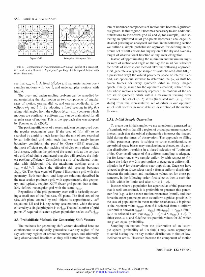
The maximum tracking error between a search grid of shift vec-tors and a real distribution of orbits depends on the geometry ofthe search grid. Consider the grid spacing of a geometricallyregular search grid in the plane defined by the total changesin RA and DEC made by moving sources during the observa-tions, which we will refer to as the (dα, dδ) plane. If the pointsof the search grid are arrayed at the vertices of identical adjoin-ing geometric cells on the (dα, dδ) plane, the point most distantfrom any point on the search grid is the point at the center ofeach cell. The distance from any vertex of a cell to the center ofthat cell defines the maximum tracking error of that search grid.

For points arrayed on the vertices of a grid of adjoining rect-angles with sidelengths dA and dB, the maximum tracking erroris ϵmax ¼ 1

2

ffiffiffiffiffiffiffiffiffiffiffiffiffiffiffiffiffiffiffiffiffiffidA2 þ dB2

p. In the case where dA ¼ dB, this be-

comes ϵmax ¼ffiffiffi2

pdA=2. This geometry well approximates the

search grids used by most previous surveys. The left panelof Figure 1 illustrates a grid with this geometry.

If a fixed (d _θ,dϕ) grid spacing is adopted such that a max-imum tracking error ϵmax is satisfied after time t for objects withangular rate of motion _θ ¼ _θ0, objects with _θ > _θ0 will see in-creasing tracking errors. To illustrate, consider a roughly rectan-gular grid where dA≃ d _θt and dB≃ 2_θt sinðdϕ=2Þ. Insertingthese values into our definition of ϵmax for a rectangular grid, we

PENCIL-BEAM SURVEYS FOR TRANS-NEPTUNIAN OBJECTS 551

2010 PASP, 122:549–559



see that ϵmax ∝ _θ. A fixed (d _θ,dϕ) grid parameterization over-samples motions with low _θ, and undersamples motions withhigh _θ.

The over- and undersampling problem can be remedied byparameterizing the sky motion as two components of angularrates of motion, one parallel to, and one perpendicular to theecliptic ( _θ∥ and _θ⊥). By adopting a fixed spacing in ( _θ∥, _θ⊥)along with angles from the ecliptic (ϕmin, ϕmax) between whichmotions are confined, a uniform ϵmax can be maintained for allangular rates of motion. This is the approach that was adoptedby Fuentes et al. (2009).

The packing efficiency of a search grid can be improved overthe regular rectangular case. If the area of (dα, dδ) to besearched by a grid is much larger than the unit of area searchedby an individual grid point such that we can largely ignoreboundary conditions, the proof by Gauss (1831) regardingthe most efficient regular packing of circles on a plane holds.In this case, defining the points of the search grid as the verticesof a grid of adjoining equilateral triangles will produce the high-est packing efficiency. Considering a grid of equilateral trian-gles with sidelength dA, the maximum tracking error isϵmax ¼ dA=

ffiffiffi3

p(where the effective dB spacing becomes

3ϵmax=2). The right panel of Figure 1 illustrates a grid with thisgeometry. Both our short- and long-arc solutions described inthe next section produce a grid with approximately this geome-try, and typically require ≥20% fewer grid points than a simi-larly defined rectangular grid with the same ϵmax.

Regardless of the grid geometry, each cell is basically cover-ing a small area of the final (dα, dδ) plane. The final area of the(dα, dδ) plane covered by real objects is approximately ∝t2

(equations [3] and [4], neglecting acceleration), while the areacovered by a single grid point is∝ϵ2max. The total number of gridpointsN required to search a given population scales as t2=ϵ2max.

2.3. Probabilistic Methods for Generating Shift Vectors

The methods for generating shift vectors described here arecumbersome to analytically generalize over any region of thesky, arbitrary regions of orbital parameter space, and arbitrarilylong observational baselines as they still suffer from the prob-

lem of nonlinear components of motion that become significantas t grows. In this regime it becomes necessary to add additionaldimensions to the search grid (€θ and _ϕ, for example), and se-lecting an optimized set of grid-points becomes a challenge. In-stead of pursuing an analytical solution, in the following sectionwe outline a simple probabilistic approach for defining an op-timum set of shift vectors for any region of the sky and over anylength of observational baseline at any solar elongation.

Instead of approximating the minimum and maximum angu-lar rates of motion and angle on the sky for an ad hoc subset ofthe orbits of interest, our method takes the following approach:First, generate a very large sample of synthetic orbits that fill (ina prescribed way) the orbital parameter space of interest. Sec-ond, use ephemeris software to determine the (α, δ) shift be-tween frames for every synthetic orbit in every imagedepoch. Finally, search for the optimum (smallest) subset of or-bits whose motions accurately represent the motions of the en-tire set of synthetic orbits within a maximum tracking errortolerance. The set of (α, δ) shifts (translated into [x, y) pixelshifts] from this representative set of orbits is our optimumset of shift vectors. A more detailed description of the methodfollows.

2.3.1. Initial Sample Generation

To create our initial sample, we use a randomly generated setof synthetic orbits that fill a region of orbital parameter space ofinterest such that the orbital ephemerides intersect the imagedfield during the times of observation. The approach to fillingorbital parameter space is subject to some consideration, asany orbital-space biases may translate into a skewed on-sky mo-tion distribution, resulting in a biased selection of “optimum”orbits. Over small ranges of d, a uniform sampling is adequate,but for larger ranges we sample uniformly with respect to d�c,where the index c ¼ 2 is appropriate to generate a uniform dis-tribution in _θ for observations near opposition. Once we haveselected a given d, we select a and e from a uniform distributionbetween the minimum and maximum values set for those pa-rameters, in the following order: first select e, then a such thatit falls within its limits and also a ≥ dð1� eÞ.

In cases where a population has a particular orbital parameterthat is well-constrained, it is preferable to generate this param-eter first (e.g., a for a mean-motion resonance [mmr]), and thenforce the other parameters onto as uniform a grid as possible. Inthe case of populations in mean-motion resonances, a is pinnedat the resonant value ammr, then d is selected from a uniformdistribution between ammrð1� emaxÞ and ammrð1þ emaxÞ. Final-ly, e is selected such that ammrð1� eÞ ≤ d ≤ ammrð1þ eÞ. Ineither case, a, e, and d define two possible values for M, whichare given equal probability.

Sampling inclination from the distribution of an isotro-pic sphere (probability of i ∝ sinðiÞ) may seem appropriateto avoid biasing the on-sky motion distribution to that of low-inclination orbits. However, because the component of motion

FIG. 1.—Comparison of grid geometries. Left panel: Packing of a square lat-tice, with scales illustrated. Right panel: packing of a hexagonal lattice, withscales illustrated.


2010 PASP, 122:549–559



perpendicular to the ecliptic is roughly∝ sinðiÞ, and because thesmall area of any imaged field with respect to the entire skyplaces stronger limits on the phase-space volume available tohigh-inclination objects compared to low-inclination objects,we contend that is preferable to sample i from a uniformdistribution. The minimum inclination orbit possible to beobserved is imin ¼ arccosðlminÞð1� 1

dÞ, where lmin is the mini-mum ecliptic latitude of the field. In the case where retrogradeorbits are of interest, duplicate the set of inclinationswith ir ¼ 180� i.

The remaining orbital elements to be generated are the nodeand the argument of perihelion. These can be rotated to force theobject to fall on the imaged field during the dates of observation,and should fill the parameter space set by these constraintssmoothly. M and the argument of perihelion are coupled forobjects in mean-motion resonances, but for the purposes pre-sented here it is convenient to simplify the treatment by treatingthe two as independent.

Depending on the size of the orbital region of interest and thelength of the observational arc, the number of synthetic orbitsrequired to produce a statistically adequate sample varies. Thebasic requirement is that the density of points in the final (dα,dδ) plane is such that the max spacing between any two nearestneighbors in the initial sample is ≪ϵmax, ensuring that there areno empty bins in (dα, dδ) given circular bins with radius ϵmax. Intrials, we found that this required the initial sample size to rangefrom several thousand to hundreds of thousands of syntheticorbits.

Once a set of synthetic orbits has been created, the shift vec-tors for each orbit can be determined. We define the shift vectorfor orbit k in image i to be a point in the (dαi, dδi) as given byvk;i in equation (8). The list of shift vectors ½vk;0…n� is stored as alist linked to the orbit k for which they were generated. We thencompare each list of shift vectors to determine the optimum set,which is the smallest subset of vectors having motions that ac-curately represent the whole set within some spatial tolerance inthe image plane. We set this tolerance by specifying that all syn-thetic orbits in the initial sample must be matched to the motionsof at least one orbit in the optimum sample to within our max-imum tracking error tolerance ϵmax in every imaged epoch. Inother words, every synthetic orbit k must be matched to at leastone optimum orbit h in every image i by jvk;i � vh;ij ≤ ϵmax.

2.3.2. Short-arc Solution

For observational baselines over which any nonlinear com-ponent of motion is negligible compared to e, the largest offsetbetween any orbit and the nearest predicted motion vector willalways occur in the final image n. To generate shift vectors inthis regime, we use the following approach:

1. Propagate all synthetic orbits in the initial sample forwardto the final image (n) plane and record the final shift vector vk;nfor each orbit k. Find the median of the distribution of shift vec-

tors and set the corresponding point in (dαn, dδn) to be the cen-ter of a geometrically-optimum triangular grid with sidelengthdA ¼ ffiffiffi

3p

ϵmax that extends over a region of (αn, dδn) signifi-cantly larger than that occupied by any synthetic orbits inthe initial sample.

2. From this initial large grid, select only those grid pointsthat have one or more synthetic orbits whose final shift vectorlies within ϵ of it in (dαn, dδn). Record a list of the orbits that arematched to each grid point.

3. After the initial grid has been cut down to just those gridpoints that are matched to at least one synthetic orbit, find thesmallest subset that are matched to unique synthetic orbits: First,select the grid point that is matched to the largest number ofsynthetic orbits, set it and its list of orbits aside, then removethe references to each synthetic orbit recovered by that gridpoint from all other grid points. Repeat this process for the re-maining grid points, until all the original synthetic orbits areaccounted for in the set-aside list. All set-aside grid pointsare now identified as the optimum set for recovering the ini-tial sample of synthetic orbits, given this grid geometry andorientation.

4. Iterate Steps 1–3 several times, each time rotating the ini-tial grid around its central point by some small angle dμ (up to atotal rotation of 60°). Record the number of optimum grid pointsrequired for each orientation, and select the orientation that re-quires the fewest. As a small refinement, if any of the optimumgrid points are found to lie with centers outside the distributionof synthetic orbits in the (dαn, dδn) plane, we shift its center tothe nearest (dαn, dδn) point from a synthetic orbit. After thisrefinement, the set of optimum grid points from this orientationis defined as our final optimum set.

These grid points are points in the final (dα, dδ) plane. Wecan back out the implied set of optimum ( _θα, _θδ) rates by simplydividing the respective components of each grid point by thetotal observational baseline tb.

The rotation in Step 4 is included to address boundary con-ditions. If the region of (dα, dδ) searched by a grid is not≫ϵmax,then there will be a preferred orientation of the grid. However, ifϵmax is small relative to the total region, this step is unnecessary.

If, instead of trimming the search grid to as small a number ofpoints as possible, it is preferable to create a “safe” grid thatoversearches the boundaries in rate-space by some comfortablemargin, then modify Step 2 to select grid points that lie within alarger distanceN × ϵmax of any final shift vector. Step 3 must beskipped in this case. This maintains the grid spacing and geom-etry, but adds a “buffer” region around each synthetic orbit.

2.3.3. Long-arc solution

In the case that the observational baseline tb is long enoughsuch that nonlinear components of motion are nonnegligiblewith respect to ϵ, a different treatment is required. Instead ofpresuming that the largest offset between the motions of a given


2010 PASP, 122:549–559



orbit and the nearest grid point will occur in the final frame n,we must instead ensure that for every synthetic orbit there is onenonlinear shift vector which matches its motions within ϵ inevery frame. While nonlinear components of motion are non-negligible, the dominant factor driving the number of shift vec-tors required is still the linear components of motion.

1. After creating an initial sample of synthetic orbits, gener-ate a search grid via the short-arc (linear) solution for the ob-servations. When generating the search grid, set the effectivemaximum tracking error to be slightly smaller than the desiredfinal maximum tracking error. This is to take into account thatthe final grid will be selected from a discrete distribution;namely, the motions of the synthetic orbits in the initial sample.

2. For each grid point p on the optimum linear search grid,take the list lp of orbits uniquely matched to that grid point andconsider their shift vectors in every imaged epoch. For each or-bit k in list lp, find all the other orbits within lp that have motionsthat are matched to the motion of k within the desired maximumtracking error ϵmax in every frame.

3. Select the single synthetic orbit k1 with motions matchedto the largest number of unique synthetic orbits in lp and set itaside as an optimum orbit.

4. If some of the orbits linked to the grid point p are not re-covered by the first optimum orbit k1, remove all orbits recov-ered by the orbit k1 from consideration, then repeat Step 3 toselect a second optimum orbit k2.

5. Repeat Step 4 until all of the orbits linked to the grid pointp are accounted for by one or more optimum orbits.

6. Repeat Steps 2–5 for each grid point in the initial solution.

The shift vectors of the final optimum set of orbits are thenidentified as the optimum set of nonlinear shift vectors to applyto the given data set.

2.3.4. Grid Tree: Optimization for Multinight Arcs

Other significant optimizations can be made to reduce thetotal number of pixel additions required to search a given dataset. One particular optimization that our probabilistic methodlends itself to is the use of a multilevel grid tree describedby Allen (2002). This approach recognizes that for multinightstacks, there are essentially two distinct timescales: the unit timeperiods over which images are obtained (length of a singlenight), and the total observational baseline. Allen (2002) pointsout that a significant reduction in total number of required shiftvectors can be obtained if, instead of combining all images ob-tained over several nights with one search grid, images are com-bined on a per-night basis (with a single-night grid), then thesestacks are combined with a second search grid to remove themotion that would have occurred over the entire period. Ifall else remains equal, this tree-of-grids structure results in few-er overall pixel additions, as redundant combinations of imagestaken on a single night are only performed once. Since thismethod relies on combining images that are the combination

of other images, it can only be applied for combination algo-rithms that can nest: for example, weighted averaging andco-adding are usable, but not medians.

It is important to note that in combining a tree of grids, theresulting maximum tracking error ϵmax goes as the sum of eachlevel’s tracking errors

Pϵi. As such, each level’s tracking error

must be limited to ϵi ¼ ϵmax=N , where N is the total number oflevels. In the case described here, the tree has two levels, and sothe effective tracking error in each level must be limited toϵi ¼ ϵmax=2. Thus, while this two-level case requires fewer pixeladditions, it results in significantly more pixels to search than inthe one-level case.

While we have not implemented this method, we can esti-mate its results. Since the number of grid points N is approxi-mately proportional to t2=ϵ2, and the two-level case requiresϵi ¼ ϵmax=2, we can estimate that this method will require 4times as many shift vectors per unit time interval as a one-levelgrid. If we consider n nights of data, where the length of a nightis equal to the length of a day such that the total observationalbaseline is tb ¼ ð2n� 1Þ in units of the length of a single night.Thus, if the one-level grid requires N1 shift vectors for the fullobservational time line, we can estimate that the two-level gridfor the full length of time will require N2;full ≃ 4N1. The two-level method will require ∼4 times more pixels be searched inthe final stacks than the one-layer method. However, to deter-mine the improvement in pixel additions, we need to determinethe size of each nightly grid:

N2;nightly ≃N2;full

t2b≃ 4N1

ð2n� 1Þ2 : (10)

For surveys where the number of observations taken per nightNobs ≫ N2;full=N2;nightly ¼ ð2n� 1Þ2 such that the number ofpixel additions is dominated by the nightly stacks, we can es-timate the total number of pixel additions required by:

N2;add ≃N2;nightlyNpixelsNobsn≃ 4N1NpixelsNobsn

ð2n� 1Þ2 : (11)

Whereas for the one-level grid, the number of pixel additionsrequired is N1;add ¼ N1NpixelsNobsn. The resulting improve-ment in the number of required pixel additions is roughly

N1;add

N2;add≃ ð2n� 1Þ2

4: (12)

So for a two-night arc, we estimate a factor of ∼2:25 improve-ment in the number of pixel additions, while for a three-nightarc this increases to ∼6:25.


2010 PASP, 122:549–559



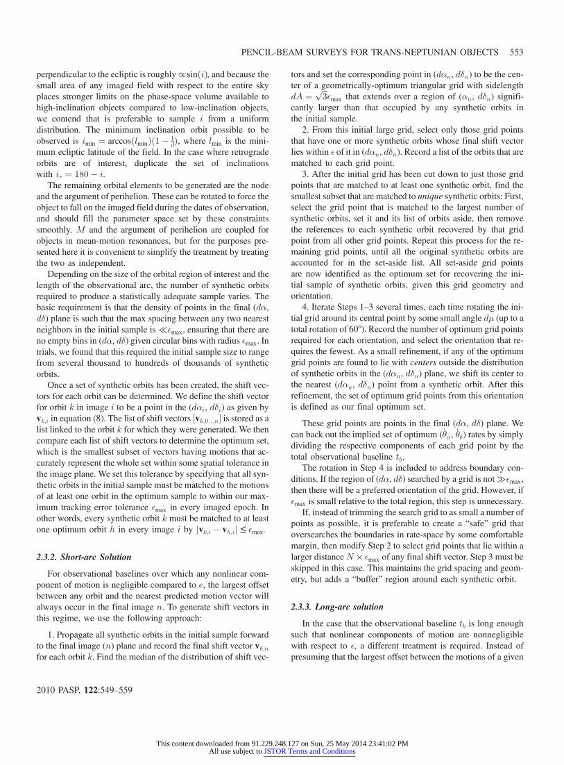
FIG. 2.—Results from survey simulations. Top panels: Fraser et al. 2008. Middle panels: Fraser & Kavelaars 2009. Bottom panels: Fuentes et al. 2009. Gray dis-tributions represent density in (dα, dδ) of synthetic orbits generated as described in text. Left panels include overlay of each survey’s search grid. Middle panels includeoverlay of our derived “optimum” search grid. Right panels show inner and outer limits in heliocentric distance d vs. inclination i derived for each survey. Cross-hatchedregion represents limit variation due to eccentricity. Black triangle represents the distance at discovery and inclination of 2008 KV42.

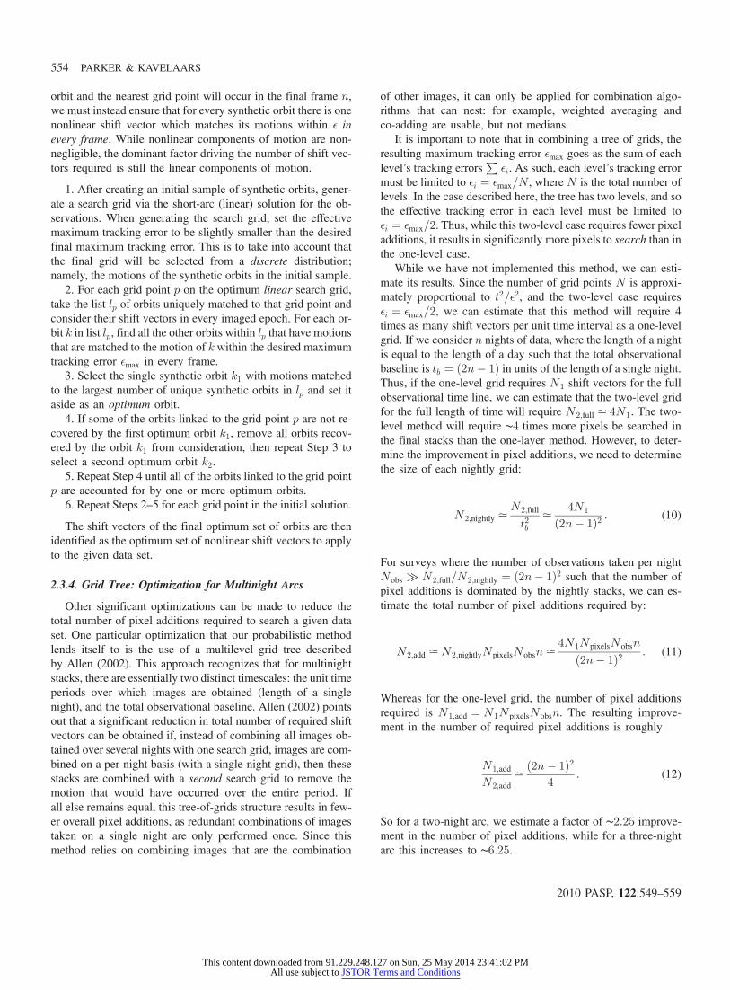
TABLE 1

SURVEY PARAMETERS

Survey and Method Baseline and Tracking Error Grid Limits Spacing Ngrid

Fraser et al. 2008 . . . . . . . . . . . . . . . . . . . . tb ∼ 4 hr 1:4″ hr�1 < _θ < 4:1″ hr�1 d _θ ¼ 0:7″ hr�1 25(searched by eye) . . . . . . . . . . . . . . . . . . . . ϵ ¼ 1:6″, F ≃ 0:57a �10° < ϕ < þ10° dϕ ¼ 5°

Fraser & Kavelaars 2009 . . . . . . . . . . . . tb ∼ 4 hr 0:4″ hr�1 < _θ < 4:5″ hr�1 d _θ ¼ 0:21″ hr�1 95(searched by eye) . . . . . . . . . . . . . . . . . . . . ϵ ¼ 1:25″, F ≃ 0:61a �15° < ϕ < þ15° dϕ ¼ 7:5°

Fuentes et al. 2009 . . . . . . . . . . . . . . . . . . tb ∼ 8:5 hr 0:7″ hr�1 < _θ∥ < 5:1″ hr�1 d _θ∥ ¼ 0:1″ hr�1 736(automated detection) . . . . . . . . . . . . . . . . ϵ ¼ 0:6″, F ≃ 0:76a �1:4″ hr�1 < _θ⊥ < þ1:4″ hr�1 d _θ⊥ ¼ 0:1″ hr�1

�15° < ϕ < þ15°

a Maximum S/N degradation factor due to tracking error, from equation (7). S=N 0 ¼ F × S=N0


2010 PASP, 122:549–559



3. COMPARISON OF PROBABILISTIC SOLUTIONTO PREVIOUS SURVEY GRIDS

In § 3.1, we will apply our probabilistic shift-vector genera-tion method to previous surveys’ observations, and compare theresults to the methods used by the authors of the surveys. Inorder to determine the limits of parameter space searched byeach survey, we generate our initial sample of synthetic orbitsover very large ranges of heliocentric distance (20–500 AU),inclination (0°–180°), and eccentricity (0–0.999). The sky mo-tion of each synthetic orbit generated is then tested to ensure thatit is within the ( _θ, ϕ), or ( _θ∥ , _θ⊥) ranges searched by the authors;as such, we only perform this characterization for surveys forwhich we can accurately reproduce the original search grid fromthe literature.

Three surveys are selected for comparison: Fraser et al. 2008,Fraser & Kavelaars 2009, and Fuentes et al. 2009. These sur-veys are selected because they cover relatively large areas(0:25–3 deg2) to relatively faint limits (R ∼ 26–27), and becausethey contain very complete information regarding their respec-tive search grids and targeted orbital parameter space, which areoutlined in Table 1. The comparisons between the original andoptimized grids and the heliocentric distance range our anal-ysis indicates each survey was sensitive to are listed in Table 2.

3.1. Fraser et al. 2008

Fraser et al. 2008 searched ∼3 deg2 (taken over baselinesranging from 4 to 8 hr) for TNOs using fixed grids of ratesand angles, searching the final stacks by eye. The images wereacquired from several facilities, and detailed grid information isonly supplied for the MEGAPrime observations. These obser-vations spanned ∼4 hr, and the search grid applied (describedin Table 1) required 25 rates and angles be searched. Theadopted search-grid spacing was fixed in d _θ and dϕ, resultingin a maximum tracking error as a function of _θ as described in§ 2.1. We estimate that the resulting maximum tracking errorwas ∼1:6″ ≃ 2:2Γ, resulting in a maximum S/N degradation fac-tor of F ≃ 0:57. As the authors reported no sensitivity loss as afunction of rate of motion, we adopt this as our uniform max-imum tracking error. The authors state that their selection ofrates and angles were designed to detect objects on circular or-bits with heliocentric distances from ∼25–100 AU with inclina-tions as high as 70°.

Due to the short arc and large tracking error of this survey,our optimum grid (with 19 shift vectors) is not radically moreefficient (∼25%) than the original grid of 25 shift vectors. Theoriginal and optimum grids, along with our initial sample, areillustrated in the left two top panels of Figure 2.

Based on our simulation of this survey, we find that the mini-mum heliocentric distance the original grid is sensitive to is astrong function of inclination, with dmin ≃ 22 AU for i ¼ 0° or-bits, climbing to dmin ≃ 30 AU for i ¼ 70°. This grid is in factsensitive to inclinations as high as 180° outside of 36 AU. The

outer edge is similarly modified by inclination, but in all casesgreater than the 100 AU goal: at the lowest, it is sensitive toobjects at distances as high as 164 AU for i ∼ 0°, and at its high-est it is sensitive to objects as distant as 184 AU for i ∼ 180°.These limits are illustrated in the top right panels of Figure 2.

3.2. Fraser & Kavelaars 2009

Fraser & Kavelaars 2009 searched ∼0:25 deg2 (takenover a ∼4 hr baseline) for TNOs with a grid of 95 rates and an-gles, aiming to be sensitive to objects on circular orbits withheliocentric distances from ∼25–200 AU. As in Fraser et al.2008, the adopted search-grid spacing was fixed in d _θ anddϕ, and the final stacks were searched by eye. The authors statethat they choose the (d _θ, dϕ) spacing to limit the maximumtracking error to ∼2Γ; we verify that at maximum _θ after4 hr, the maximum tracking error of this search grid is approxi-mately 1:25″ ∼ 1:8Γ, resulting in a maximum S/N degradationfactor of F ≃ 0:61. As the authors reported no sensitivity loss asa function of rate of motion, we adopt this as our uniform max-imum tracking error.

Based on our simulation of this survey, we find that the orig-inal search grid is overambitious, as the high-ϕ regions of thegrid are not populated by any real objects. No bound orbits ob-served on the ecliptic at opposition with heliocentric distanceoutside of d > 28 AU can have angles of motion as high as15° from the ecliptic (equation [5]). This, coupled with the over-sampling at low _θ, relative to the maximum tracking error of1.25″, resulted in excess shift vectors compared to our optimumsolution. The optimum grid requires 28 shift vectors, which rep-resents an improvement of over a factor of 3 compared the 95shift vectors searched by the authors. The original and optimumgrids, along with our initial sample, are illustrated in the left twomiddle panels of Figure 2.

Similar to Fraser et al. 2008, the minimum heliocentric dis-tance the original grid is sensitive to is a function of inclination,with dmin ≃ 24:5 AU for i ¼ 0° orbits, climbing to dmin ≃31 AU for i ¼ 70°. This grid was also sensitive to inclinationsas high as 180° outside of 36.5AU.The outer edge is significantlymore distant than claimed: at the lowest, it is sensitive to objectsat distances as high as 350 AU for i ∼ 0°, and at its highest, it issensitive to objects as distant as 385 AU for i ∼ 180°. Theselimits are illustrated in the middle right panels of Figure 2.

TABLE 2

SURVEY CHARACTERIZATION

Survey Nopt % Improveddmin

(AU)dmax

(AU)

Fraser et al. 2008 . . . . . . . . . . . . 19 24% 22−36 164−184Fraser & Kavelaars 2009 . . . . . 28 71% 24−37 360−390Fuentes et al. 2009 . . . . . . . . . . 494 33% 21−33 220−245


2010 PASP, 122:549–559



3.3. Fuentes et al. 2009

Fuentes et al. 2009 searched 0:25 deg2 (taken over a ∼8 hrbaseline) for TNOs with a grid of 732 rates parallel and perpen-dicular to the ecliptic, aiming to be sensitive to objects with he-liocentric distances from ∼20–200 AU. The large number ofresulting stacks necessitated the use of an automated detectionpipeline. Their grid spacing was d _θ∥ ¼ d _θ⊥ ¼ 0:1″ hr�1 andmotions were limited to �15° from the ecliptic. Over an ∼8 hrobservational baseline, this grid spacing translates into a maxi-mum tracking error of ϵ≃ 0:6″ ∼ 0:8Γ, resulting in a maximumS/N degradation factor of F ≃ 0:76.

Like Fraser & Kavelaars 2009, this survey also oversearcheshigh-ϕ motions. Because of the small tracking error and non-optimum grid geometry, any small oversearched regions trans-late into a significant number of additional search vectors. Theoptimum grid requires 494 shift vectors, which represents animprovement of ∼33% over the original search grid. The origi-nal and optimum grids, along with our initial sample, are illu-strated in the left two middle panels of of Figure 2.

Similar to Fraser et al. 2008, the minimum heliocentric dis-tance the original grid is sensitive to is a function of inclination,with dmin ≃ 21:5 AU for i ¼ 0° orbits, climbing to dmin≃26:5 AU for i ¼ 70°. This grid was also sensitive to inclinationsas high as 180° outside of 33.5 AU. The outer edge is signifi-cantly more distant than claimed: at the lowest, it is sensitive toobjects at distances as high as 220 AU for i ∼ 0°, and at its high-est it is sensitive to objects as distant as 245 AU for i ∼ 180°.These limits are illustrated in the bottom right panels of Figure 2.

4. EXAMPLE OF APPLICATION: LSSTDEEP FIELDS

A component of the LSST survey strategy will be to point toa single field and take hundreds of ∼30 s exposures, then latercombine them in software to search for faint moving objects(Chesley et al. 2009). On a single winter night, a single9.6deg2 field at opposition can be observed for roughly 8 hr,resulting in 850 images with a combined depth of r0 ∼ 28.We will determine the feasibility of stacking multiple nights

of data to search for specific TNO populations at even faintermagnitudes.

We have run simulations of similar LSST observations todemonstrate the utility of our method for generating shift vec-tors. One of this method’s chief advantages is the ability tostrictly limit the orbital parameters of interest, being certainto sensitize the resulting stacks only to those orbits of interestwithout creating stacks at extraneous rates of motion. As such,the simulation described here is designed to detect a populationthat has some orbital parameters that are well-defined; namely,objects in the Neptune 2:1 resonance, or “twotinos.” The orbitalranges used to simulate this population are listed in Table 3.

We compare observations made at opposition to those madeat 45° away from opposition, which have increasing contribu-tions from nonlinear components of motion. If an oppositionfield can be observed for 8 hr on a single night, fields at thiselongation can be observed for ∼7 hr per night. We simulateobserving both fields for one, two, and three nights, resultingin the total observational baselines listed in Table 4. The seeingis assumed to be the projected 75th percentile in r0, roughly0.89″ (Tyson et al. 2009). We adopt ϵmax ¼ 0:8Γ, similar to thatused in previous automated-detection-based pencil-beam sur-veys, resulting in ϵmax ≃ 0:7″.

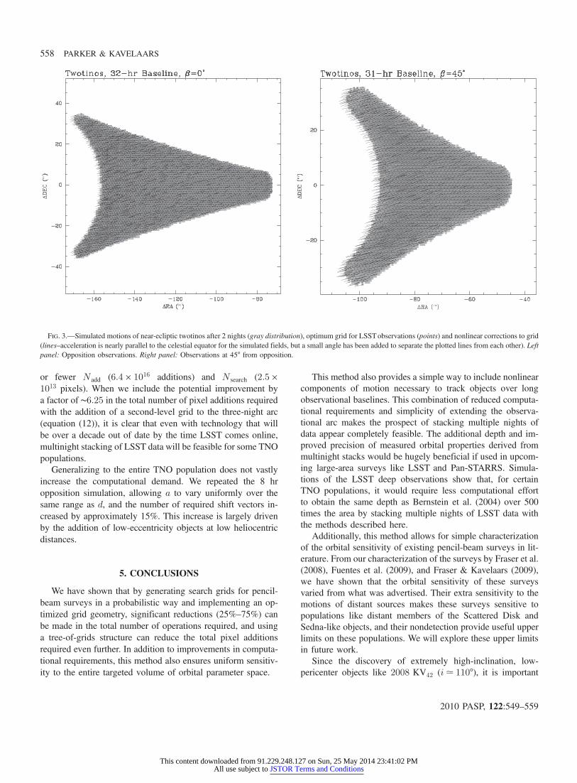
Table 4 contains the results of our simulations. We have es-timated the required number of shift vectors, pixel additions,and pixels to search (without the additional optimization fromthe tree of grids discussed in § 2.3.4). Figure 3 illustrates theoptimum nonlinear grids generated for both elongations. Alsoillustrated is the magnitude of the error between the final posi-tions of real sources and the linear extrapolation of their positionfrom their initial motion ( _θ0 , ϕ0).

It is useful to compare the total required number of pixeladditions (Nadd) and pixels to search (N search) to the mostcomputationally-intensive digital-tracking survey to date. TheHST survey performed by Bernstein et al. (2004) requiredNadd ∼ 1016 additions and N search ∼ 7 × 1013 pixels with 2004computer technology. Because the LSST psf is significantlylarger than that of HST, fewer shift vectors are required forthe same observational baseline. In our LSST Twotino simula-tions, even the three-night opposition solution requires as many

TABLE 3

LSST SIMULATION ORBITS

Twotinos

Parameter Range Distribution

a . . . . . . . . . 42.8 AU Single-valuedq . . . . . . . . . 25a–42.8 AU Uniforme . . . . . . . . . 0–0.416 Uniformd . . . . . . . . . 25a–60.6 AU pðdÞ ∝ d�2

i . . . . . . . . . . 0°–45° Uniform

a Minimum q and d selected to prevent interactions withUranus.

TABLE 4

LSST SIMULATION RESULTS

Twotinos

βtb(hr)

Depth(r0 mag) N shift Nadd Nsearch

0° . . . . . . . . 8 28 200 5:4 × 1014 6:4 × 1011

32 28.4 3,359 1:8 × 1016 1:1 × 1013

56 28.6 7,743 6:4 × 1016 2:5 × 1013

45° . . . . . . . 7 27.9 113 2:7 × 1014 3:6 × 1011

31 28.3 1,965 9:4 × 1015 6:3 × 1012

54 28.5 6,864 4:9 × 1016 2:2 × 1013


2010 PASP, 122:549–559



or fewer Nadd (6:4 × 1016 additions) and N search (2:5×1013 pixels). When we include the potential improvement bya factor of ∼6:25 in the total number of pixel additions requiredwith the addition of a second-level grid to the three-night arc(equation (12)), it is clear that even with technology that willbe over a decade out of date by the time LSST comes online,multinight stacking of LSST data will be feasible for some TNOpopulations.

Generalizing to the entire TNO population does not vastlyincrease the computational demand. We repeated the 8 hropposition simulation, allowing a to vary uniformly over thesame range as d, and the number of required shift vectors in-creased by approximately 15%. This increase is largely drivenby the addition of low-eccentricity objects at low heliocentricdistances.

5. CONCLUSIONS

We have shown that by generating search grids for pencil-beam surveys in a probabilistic way and implementing an op-timized grid geometry, significant reductions (25%–75%) canbe made in the total number of operations required, and usinga tree-of-grids structure can reduce the total pixel additionsrequired even further. In addition to improvements in computa-tional requirements, this method also ensures uniform sensitiv-ity to the entire targeted volume of orbital parameter space.

This method also provides a simple way to include nonlinearcomponents of motion necessary to track objects over longobservational baselines. This combination of reduced computa-tional requirements and simplicity of extending the observa-tional arc makes the prospect of stacking multiple nights ofdata appear completely feasible. The additional depth and im-proved precision of measured orbital properties derived frommultinight stacks would be hugely beneficial if used in upcom-ing large-area surveys like LSST and Pan-STARRS. Simula-tions of the LSST deep observations show that, for certainTNO populations, it would require less computational effortto obtain the same depth as Bernstein et al. (2004) over 500times the area by stacking multiple nights of LSST data withthe methods described here.

Additionally, this method allows for simple characterizationof the orbital sensitivity of existing pencil-beam surveys in lit-erature. From our characterization of the surveys by Fraser et al.(2008), Fuentes et al. (2009), and Fraser & Kavelaars (2009),we have shown that the orbital sensitivity of these surveysvaried from what was advertised. Their extra sensitivity to themotions of distant sources makes these surveys sensitive topopulations like distant members of the Scattered Disk andSedna-like objects, and their nondetection provide useful upperlimits on these populations. We will explore these upper limitsin future work.

Since the discovery of extremely high-inclination, low-pericenter objects like 2008 KV42 (i≃ 110°), it is important

FIG. 3.—Simulated motions of near-ecliptic twotinos after 2 nights (gray distribution), optimum grid for LSSTobservations (points) and nonlinear corrections to grid(lines–acceleration is nearly parallel to the celestial equator for the simulated fields, but a small angle has been added to separate the plotted lines from each other). Leftpanel: Opposition observations. Right panel: Observations at 45° from opposition.


2010 PASP, 122:549–559



to understand these surveys’ sensitivity to such populations. Wenote that Fuentes et al. (2009) is the only survey characterizedhere that was sensitive to objects with the same inclination anddistance at discovery as 2008 KV42 (see Fig. 2, bottom-rightpanel), but we contend that it is unlikely that they would haverecognized any detection as belonging to this retrogradepopulation. Since follow-up has been performed only rarelyfor these deep surveys, orbital inclination and heliocentric dis-tance usually remain degenerate, with the prograde solution

lying at lower distances (though this degeneracy is rarelyacknowledged). It is possible that detections labeled as high-inclination prograde objects may in fact be objects with retro-grade orbits like 2008 KV42 at greater distance. Only multinightarcs or follow-up at later epochs can break this degeneracy andclearly identify objects belonging to rare TNO subclasses.

Alex Parker is funded by the NSF-GRFP award DGE-0836694.

REFERENCES

Allen, R. L. 2002, Ph.D. thesis, Univ. MichiganAllen, R. L., Bernstein, G. M., & Malhotra, R. 2001, ApJ, 549, L241———. 2002, AJ, 124, 2949Axelrod, T., & LSST Science Collaborations & LSST Project 2009,

LSST Science Book, Version 2.0, preprint (arXiv:0912.0201)Bernstein, G. M., et al. 2004, AJ, 128, 1364Brasser, R., Duncan, M. J., & Levison, H. F. 2006, Icarus, 184, 59Chesley, S. R., Jones, R. L., Trilling, D. E., & LSST Science Collab-

orations & LSST Project 2009, LSST Science Book, Version 2.0,preprint (arXiv:0912.0201)

Chiang, E. I., & Brown, M. E. 1999, AJ, 118, 1411Cochran, A. L., Levison, H. F., Stern, S. A., & Duncan, M. J. 1995,

ApJ, 455, 342Denneau, L., Kubrica, J., & Jedicke, R. 2007, ASP Conf. Ser. 376,

ADASS XVI, 257

Fraser, W. C., et al. 2008, Icarus, 195, 827Fraser, W. C., & Kavelaars, J. J. 2009, AJ, 137, 72Fuentes, C. I., George, M. R., & Holman, M. J. 2009, ApJ, 696, 91Gauss, C. F. 1931, Gottingsche Gelehrte Anzeigen, 2, 188Gladman, B., & Kavelaars, J. J. 1997, A&A, 317, L35Gladman, B., Kavelaars, J. J., Nicholson, P. D., Loredo, T. J., & Burns,

J. A. 1998, AJ, 116, 2042Gladman, B., Kavelaars, J. J., Petit, J. M., Morbidelli, A., Holman, M.,

& Loredo, T. 2001, AJ, 122, 1051Luu, J. X., & Jewitt, D. C. 1998, ApJ, 502, L91Tyson, J. A., Guhathakurta, P., Bernstein, G. M., & Hut, P. 1992,

BAAS, 24, 1127Tyson, J. A., Gee, P., Thorman, P., & LSST Science Collaborations &

LSST Project 2009, LSST Science Book, Version 2.0, preprint(arXiv:0912.0201)


2010 PASP, 122:549–559

