Munich Personal RePEc Archive

Relationship between macroeconomic

variables and stock market index:

evidence from India

Pathan, Rubina and Masih, Mansur

INCEIF, Malaysia, INCEIF, Malaysia

10 July 2013

Online at https://mpra.ub.uni-muenchen.de/63302/

MPRA Paper No. 63302, posted 28 Mar 2015 15:37 UTC

Relationship between macroeconomic variables and stock market index:

evidence from India

Rubina Pathan 1 and Mansur Masih2

Abstract

The purpose of this paper is to study the direction of causality between the stock market and

macroeconomic variables. India is taken as a case study. Although, there have been many

studies which attempted to find out the relationship between Indian stock market and

economic variables, this paper is a fresh attempt to investigate the cointegrating relationship

and Granger-causality between the variables. The paper considers the monthly data of

major macroeconomic variables which are interest rate, money supply, wholesale price

index, and exchange rate and also an important variable for any stock market and economy

which is Foreign Institutional investment. Our findings provide evidence of a stable long run

equilibrium relationship between the stock market and economic growth in India. The study

reconfirms the traditional belief that the real economic variables continue to affect the stock

market in the post-reform era in India and also highlights the insignificance of certain

variables with respect to stock market. The study also discerns the Granger-causal chain

among the variables. This has an important policy implication for the national policy makers,

researchers, corporate managers and regulators.

1 Rubina Pathan, Graduate student in Islamic finance at INCEIF, Lorong Universiti A, 59100 Kuala Lumpur, Malaysia.

2 Corresponding author, Professor of Finance and Econometrics, INCEIF, Lorong Universiti A, 59100 Kuala Lumpur,

Malaysia. Phone: +60173841464 Email: mansurmasih@inceif.org

Relationship between macroeconomic variables and stock market index:

evidence from India

1.1 Introduction

Indian economy is the third largest economy in the world in terms of purchasing power. It is

going to touch new heights in coming years. As predicted by Goldman Sachs, the Global

Investment Bank, by 2035 India would be the third largest economy of the world just after

US and China. It will grow to 60% of size of the US economy. This booming economy of

today has to pass through many phases before it can achieve the current milestone of 9%

GDP.3 Looking at the growth prospect and importance of the economy, we decided to take

India as a country of study for this paper.

For economists, policy makers and even the investors, it is important to know the factors that

influence the behavior of stock prices and also the development and growth of the economy.

The inter dependence of macroeconomic factors has attracted the attention of economists,

policy makers, and the investment community for a long time. The knowledge of these inter

relationships between the stock market and the macroeconomic factors are of critical

importance, not merely to the industry players, but to the macroeconomic policy makers as

well. The well being of an economy as well as the depth in the capital markets is crucial or

the development of a robust real sector in the system and the development of any country.

There have been countless researches in the field of the relationship between the Stock index

and individual macroeconomic variables, encompassing both the developed as well as the

emerging economies to show the importance of finding out cointegration between these

variables.

The issue whether the stock market performance leads or follows economic activity is

important to find out. Almost all the indicators such as market capitalization, trading volume,

total turnover and the market index have shown tremendous growth in past few years. These

developments are often claimed by the authorities to be an indication of economic progress of

the country.

Hence, It would be useful to examine BSE Index as one of the core variables have any

3http://www.sharetipsinfo.com/indian-economy.html

influence the health of the economy.

This study is an attempt to examine whether there exist any long-run and/or short-run

cointegrating relationship between stock prices and some important macroeconomic variables

namely exchanges rates, interest rates, money supply, Foreign Institutional Investment and

Inflation for India using cointegration and the Granger causality method. If stock prices and

macroeconomic variables are significantly related and the causation runs from

macroeconomic variables to stock prices then crises in stock markets can be prevented by

controlling fluctuations in macroeconomic variables (specifically, controlling exchange rates

and interest rates movements). Government can focus on domestic economic policies to

stabilize the stock market during any financial crisis.

1.0 Objectives of the study

The main objective for this study is to find if there is and the nature of the relationship

between the Bombay Stock Exchange Index (“BSE”)and some major contributing

macroeconomic variables that have proven in the past to influence the other world indices

across the region and globe. Moreover, the underlining purpose of this research is to

determine the levels of influence the Bombay Stock Exchange Index has on real

macroeconomic factors and vice versa. Macroeconomic factors under consideration are

interest rate (SBI Prime Lending Rate, (INT)), money supply (“M3”), Wholesale Price Index

(WPI “WPI”), exchange rate (US/INR“EX”).and Foreign Institutional Investment in Indian

Capital Market("FII"). The study does not assume any a prior relationship between these

variables and the stock market and is open to the possible two-way relationship between

them.

To reiterate the main objective of this study is to investigate the cointegrating relationship

between India's one of the biggest stock exchange houses, Bombay Stock Exchange Index

and macroeconomic variables in India, and also to find out whether the policy makers can

forecast economic growth using Bombay Stock Exchange.

During the last three decades there have been many studies on this relationship. However,

there is an acute need to apply more rigorous non-linear techniques as stock prices movement

is better captured in these methods. Also, there are clearly identified direct beneficiaries of

this knowledge. If academicians and practitioners know the precise macro variables that

influence the stock prices and also the nature of the relationship then understanding and

predicting stock market behaviour would be much simpler with the help of these economic

variables. Using this knowledge the policy- makers may try to influence the stock market or

the investors, managers may make appropriate investment or managerial decisions.

2.0 Literature review

There is an increasing amount of empirical evidence which has been noticed by several

researchers which leads to the conclusion that a range of financial and macroeconomic

variables can predict stock market returns

In a slightly older research of Mukherjee and Naka (1995), with the use of Johansen’s (1998)

VECM, the authors analyzed the relationship between the Japanese Stock Market and

exchange rate, inflation, money supply, real economic activity, long-term government bond

rate, and call money rate. They concluded that a cointegrating relation indeed existed and that

stock prices contributed to this relation. Maysami and Koh (2000) in a similar attempt

concluded that such relationships do exist in Singapore. They found that inflation, money

supply growth, changes in short- and long-term interest rate and variations in exchange rate

formed a cointegrating relation with changes in Singapore’s stock market levels..

Habibullah and Baharumshah (2000) used Toda and Yamamoto (1995) methodology to

establish the lead and lag relationship between Malaysian stock market and macroeconomic

variables. The study used quarterly data for the sample period 1981:1 to 1994:4. Their study

includes five macroeconomic variables namely money supply, gross national product, price

level (Consumer Price Index), interest rate (3-month Treasury bill rate) and exchange rate

(real effective exchange rate). The results of the analysis indicated that stock prices lead

nominal income, the price level and the exchange rate, but money supply and interest rate

lead stock prices.

Ibrahim and Aziz (2003) estimated vector auto-regression model to explore the dynamic

linkages between stock prices and four macroeconomic variables for the case of Malaysia.

Empirical results of the analysis suggested the presence of a long-run relationship between

these variables and the stock prices and substantial short-run interactions among them. They

also stated that the stock market is playing somewhat predictive role for the macroeconomic

variables. Chong and Koh’s (2003) in a further study concluded wit the same results showing

that stock prices, economic activities, real interest rates and real money balances in Malaysia

were linked in the long run both in the pre- and post capital control sub periods.

Dimitrova (2005) uses a multivariate, open-economy, short-run model to test the hypothesis

that in the short-run, un upward trend in the stock market may cause currency depreciation,

whereas weak currency may cause decline in the stock market. His study included stock

prices, exchange rates, domestic output, interest rates, current account balance, oil prices and

foreign output in model specification. The study uses monthly data for the United States and

the United Kingdom over the period from January 1990 to August 2004. Using OLS

regression analysis, he found a positive link between stock prices and exchange rates when

stock prices are the lead variable and likely negative when exchange rates are the lead

variable. His results provided evidence that stock prices have a positive impact on domestic

output and inflation rate is negatively associated with stock prices.

Chandra (2012) examined the direction of causality between foreign institutional investment

(FII) trading volume and stock market returns in the Indian context.in his findings Bi-

directional causality between net FII investment and Indian stock market return is observed.

In general, the FIIs seem to be chasing the Indian stock market returns. It is found that FII

trading behaviour resulting in heavy trading volumes may cause variations in stock market

returns only in the very short-term, but afterwards, it is the stock market returns which cause

changes in FII trading behaviour.

Pal and Mittal (2011) used Quarterly time series data spanning the period from January 1995

to December 2008 to examine the long-run relationship between the Indian capital markets

and key macroeconomic variables such as interest rates, inflation rate, exchange rates and

gross domestic savings (GDS) of Indian economy. their findings of the study establish that

there is co-integration between macroeconomic variables and Indian stock indices which is

indicative of a long-run relationship. The ECM shows that the rate of inflation has a

significant impact on both the BSE Sensex and the S&P CNX Nifty. Interest rates on the

other hand, have a significant impact on S&P CNX Nifty only. However, in case of foreign

exchange rate, significant impact is seen only on BSE Sensex. The changing GDS is observed

as insignificantly associated with both the BSE Sensex and the S&P CNX Nifty. The paper,

on the whole, conclusively establishes that the capital markets indices are dependent on

macroeconomic variables even though the same may not be statistically significant in all the

cases.

Vuyyuri (2005) investigated the cointegrating relationship and the causality between the

financial and the real sectors of the Indian economy using monthly observations from 1992

through December 2002. The financial variables used were interest rates, inflation rate,

exchange rate, stock return, and real sector was proxied by industrial productivity. Johansen

(1988) multivariate cointegration test supported the long-run equilibrium relationship

between the financial sector and the real sector, and the Granger test showed unidirectional

Granger causality between the financial sector and real sector of the economy.

Bhattacharya and Mukherjee (2002) tested the causal relationships between the BSE Sensex

and five macroeconomic variables applying the techniques of unit-root tests, cointegration

and long-run Granger non-causality test proposed by Toda and Yamamoto (1995). Their

major findings were that there is no causal linkage between the stock prices and money

supply, national income and interest rate while the index of industrial production leads the

stock price and there exists a two-way causation between stock price and rate of inflation.

3.0 The theory

Economic theory asserts that exchange rates, inflation, money supply and interest rates, as

well as other factors are important variables in developing a comprehensive understanding of

the behavior of stock prices and index movements.

Exchange Rates - Traditional economic models argue that changes in exchange rates affect

balance sheet items of a firm through its competitiveness as expressed in foreign currency

and ultimately, profits and equity leading to price adjustments in the capital markets. This

volatility in price adjustments of individual firms leads to the impact on the index. Branson

and Masson (1977), Ghartey (1998), Meese and Rogoff (1983), and Wolff (1988) have found

some relationship between macroeconomic variables and exchange rates.

Wholesale Price Index(WPI) – Several studies provide a negative relationship between real

stock returns and Inflation or US and European stock markets Linter (1975), Fama (1981,

1982), Fama and Schwert (1977), Geske and Roll (1983), and Caporale and Jung (1997) for

US financial market and Wahlroos and Berglund (1986) and Asprem (1989) provide for

European markets. Chatrath and Ramchander (1997) and Hu and Willett (2000) provide

evidence for Indian financial market. Keeping in mind these empirical findings we carry on

with the theoretical framework of a negative relationship between the WPI and the stock

prices.

Money Supply - Friedman and Schwartz (1963) explained the relationship between money

supply and stock returns by simply hypothesizing that the growth rate of money supply would

affect the aggregate economy and hence the expected stock returns. The growth of money

supply is directly related to the cost of money. The index on theoretical grounds has a

negative relationship. As a decrease in cost of borrowing would lead to increased leveraging

thus resulting in a price surge. An increase Money supply growth would indicate excess

liquidity available for buying securities, resulting in higher security prices. Empirically,

Hamburger and Kochin (1972) and Kraft and Kraft (1977) found a strong linkage between

the two variables, while Cooper (1974) and Nozar and Taylor (1988) found no relation.

Interest rate - Interest Rate is a rate which is charged or paid for the use of money. It is often

expressed as an annual percentage of the principal. It is calculated by dividing the amount of

interest by the amount of principal. Interest rates often change as a result of inflation and

Federal Reserve policies. This can play a vital factor in deciding the amount of savings as

opposed to borrowing. If interest rate is low, people will reduce savings in banks and invest

more money in the market indexes; therefore it is presumed that interest this may play an

important role. Since it’s difficult to find any benchmark interest rate for the entire time

period under study, we have taken the SBI Prime Lending Rate (SBIPLR) as the proxy for

the interest rate (INT) prevailing in the economy.

Bombay Stock Exchange: It is India's premier Index for which Data is available for long

period. The market capitalisation of BSE Index 5000 companies are listed on BSE of appx

5000 companies (making it world's No. 1 exchange in terms of listed members) command a

total market capitalization of USD Trillion 1.2 which constitute appx 65% of India's total

GDP of 2012 v/s 26% of India's GDP from 2002-2003. Bombay Stock Exchange is world's

fifth most active exchange in terms of number of transactions handled through its electronic

trading system. It is also one of the world’s leading exchanges (3rd largest as on July 2012)

for Index options trading. (Source: World Federation of Exchanges).4

4http://en.wikipedia.org/wiki/Bombay_Stock_Exchange

Based on the literature review and theory we decided to go further using Time Series

Analysis for our research.

4.0 Data and Methodology

5.1 Data

The data for the subsequent research is spread over monthly observations 2004 M4, to

2013M2 a total of 107 months. The data for the variables has mainly been sourced from the

Datastream.

All variables were taken in their level form, and for their log form, for running identification

tests their difference log forms have been taken in account.

5.2 Methodology

This study will use Time Series Technique to evaluate objectives. The MICROFIT software

is used for this method. By using Time Series technique, the main aim of this study is to find

out which factors are cointegrated and move together with one another in long run. The

VECM will identify the causal relationship between co integrated variables. While the VDCs

and IRF try to find the most leading variable, the persistence profile may inform us about the

duration required for co integrated variables to return back to their equilibrium when the

external shock occurs.

5.0 Estimation of the model and empirical tests

In this section paper will carry out the eight steps of the time series and explain empirically

following which there will be a segment on policy implications.

6.1 Testing for non stationary variables (Unit root test)

The first step is empirical testing by determining the stationarity of the variables used. In

order to proceed with the testing of Cointegration, ideally variables should be I (1). In their

level form they must be non-stationary, while in their first differenced form they must be

stationary. The differenced form for each variable used is created by taking the difference of

their log forms. For example, DLBSE = LBSE – LBSE(-1). It is depicted by conducting the

Augmented Dickey-Fuller (ADF) Unit Root Test and Phillip Perron Unit Root Test on each

variable in both level and differenced form.

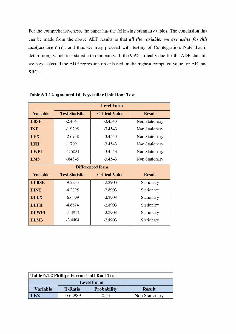
For the comprehensiveness, the paper has the following summary tables. The conclusion that

can be made from the above ADF results is that all the variables we are using for this

analysis are I (1), and thus we may proceed with testing of Cointegration. Note that in

determining which test statistic to compare with the 95% critical value for the ADF statistic,

we have selected the ADF regression order based on the highest computed value for AIC and

SBC.

Table 6.1.1Augmented Dickey-Fuller Unit Root Test

Level Form

Variable Test Statistic Critical Value Result

LBSE -2.4041 -3.4543 Non Stationary

INT -1.9295 -3.4543 Non Stationary

LEX -2.6938 -3.4543 Non Stationary

LFII -1.7091 -3.4543 Non Stationary

LWPI -2.5024 -3.4543 Non Stationary

LM3 -.84845 -3.4543 Non Stationary

Differenced form

Variable Test Statistic Critical Value Result

DLBSE -9.2233 -2.8903 Stationary

DINT -4.2895 -2.8903 Stationary

DLEX -6.6699 -2.8903 Stationary

DLFII -4.8674 -2.8903 Stationary

DLWPI -5.4912 -2.8903 Stationary

DLM3 -3.4464 -2.8903 Stationary

Table 6.1.2 Phillips Perron Unit Root Test

Level Form

Variable T-Ratio Probability Result

LEX -0.62989 0.53 Non Stationary

LBSE -1.9570 0.53 Non Stationary

LM3 -0.68252 0.496 Non Stationary

LWPI 1.2117 0.228 Non Stationary

LFII -3.2144 0.002 Stationary

INT -2.1001 0.038 Stationary

Differenced form

Variable T-Ratio Probability Result

DLEX -9.5875 0 Stationary

DLBSE -11.3543 0 Stationary

DLM3 -8.1294 0 Stationary

DLWPI -8.4848 0 Stationary

DLFII -10.1332 0 Stationary

DINT -12.0716 0 Stationary

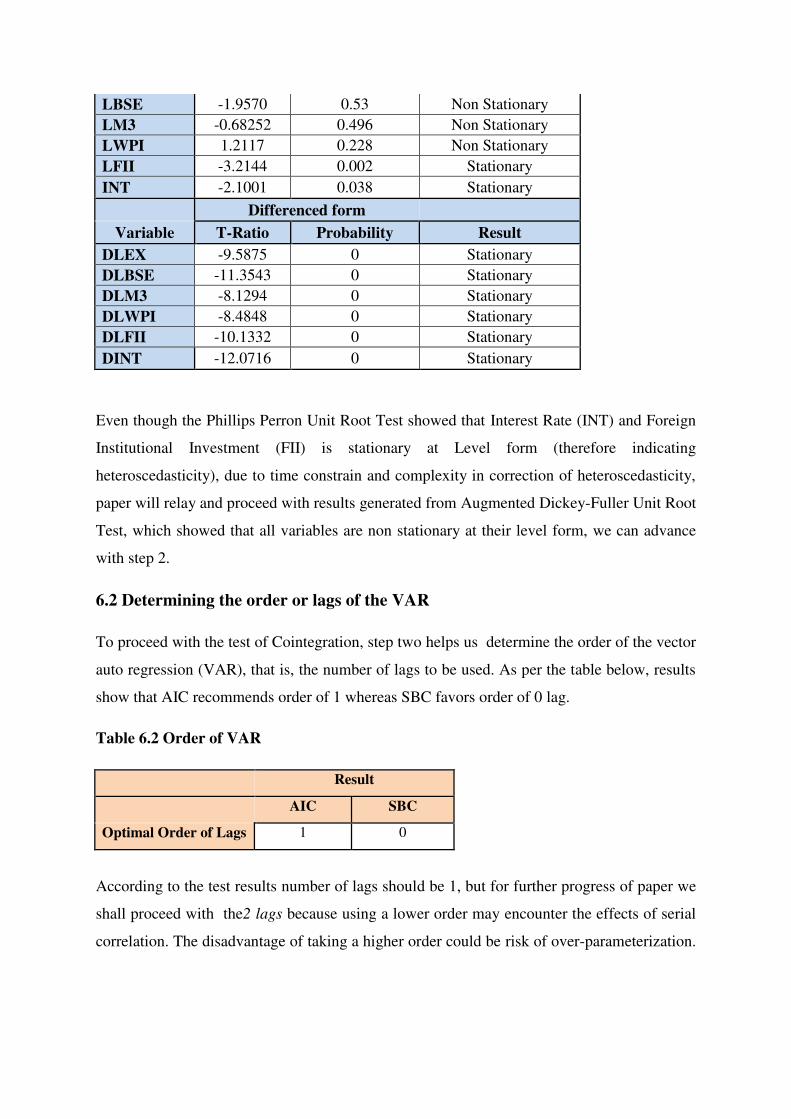
Even though the Phillips Perron Unit Root Test showed that Interest Rate (INT) and Foreign

Institutional Investment (FII) is stationary at Level form (therefore indicating

heteroscedasticity), due to time constrain and complexity in correction of heteroscedasticity,

paper will relay and proceed with results generated from Augmented Dickey-Fuller Unit Root

Test, which showed that all variables are non stationary at their level form, we can advance

with step 2.

6.2 Determining the order or lags of the VAR

To proceed with the test of Cointegration, step two helps us determine the order of the vector

auto regression (VAR), that is, the number of lags to be used. As per the table below, results

show that AIC recommends order of 1 whereas SBC favors order of 0 lag.

Table 6.2 Order of VAR

Result

AIC SBC

Optimal Order of Lags 1 0

According to the test results number of lags should be 1, but for further progress of paper we

shall proceed with the2 lags because using a lower order may encounter the effects of serial

correlation. The disadvantage of taking a higher order could be risk of over-parameterization.

But with the amount of data point available taking into consideration VAR order of 2will be

appropriate.

6.3 Cointegration Test

After completing the test of (non)stationarity by proving that the variables are I (1) and

determined the optimal VAR order as 2, the third step is to test the Cointegration. Two tests

that are performed for observing Cointegration are Engle Granger Test and Johansen Test.

Using Engle Granger Test study stationarity of Error Term (Residual). The cointegration can

be observed if the Error Term is stationary and Johansen Test. Due to time constraint we only

studied Johansen test.

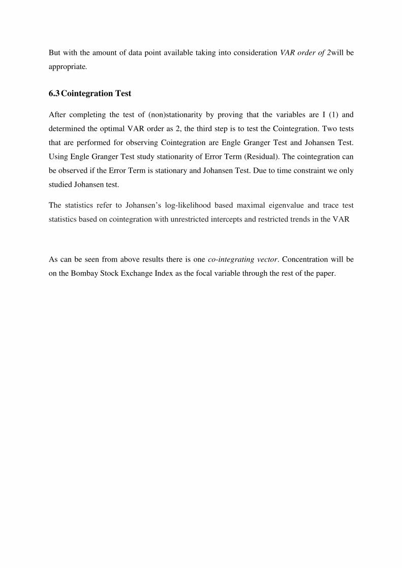
The statistics refer to Johansen’s log-likelihood based maximal eigenvalue and trace test

statistics based on cointegration with unrestricted intercepts and restricted trends in the VAR

As can be seen from above results there is one co-integrating vector. Concentration will be

on the Bombay Stock Exchange Index as the focal variable through the rest of the paper.

Table 6.3.1 Johansen Test

Table 6.3.2 Johansen Test

Ho H1 Statistic 95% Critical Value 90% Critical Value

Maximum Eigen value

Statistics

r = 0 r = 1 63.684 43.61 40.76

r<= 1 r = 2 44.2477 37.86 35.04

r<= 2 r = 3 20.1817 31.79 29.13

r<= 3 r = 4 10.72 25.42 23.1

r<= 4 r = 5 7.5283 19.22 17.18

r<= 5 r = 6 4.5535 12.39 10.55

Trace Statistic

r = 0 r = 1 150.9152 115.85 110.6

r<= 1 r = 2 87.2312 87.17 82.88

r<= 2 r = 3 42.9835 63 59.16

r<= 3 r = 4 22.8018 42.34 39.34

r<= 4 r = 5 12.0818 25.77 23.08

r<= 5 r = 6 4.5535 12.39 10.55

6.4 Long Run Structural Modeling (LRSM)

In the step four, which is Long Run Structural Modeling, paper attempts to quantify apparent

theoretical relationship among the BSE Stock Exchange (LBSE)and interest rate (INT),

money supply (LM3), Wholesale Price Index (LWPI), exchange rate (LEX) and Foreign

Institutional Investment in capital Market (LFII). The main purpose is to compare our

statistical findings with theoretical or intuitive expectations. Relying on the Long Run

Structural Modeling (LRSM) component of Microfit, and normalizing our variable of interest

the LBSE (Bombay Stock Exchange Index), we initially obtained the results in the following

table.

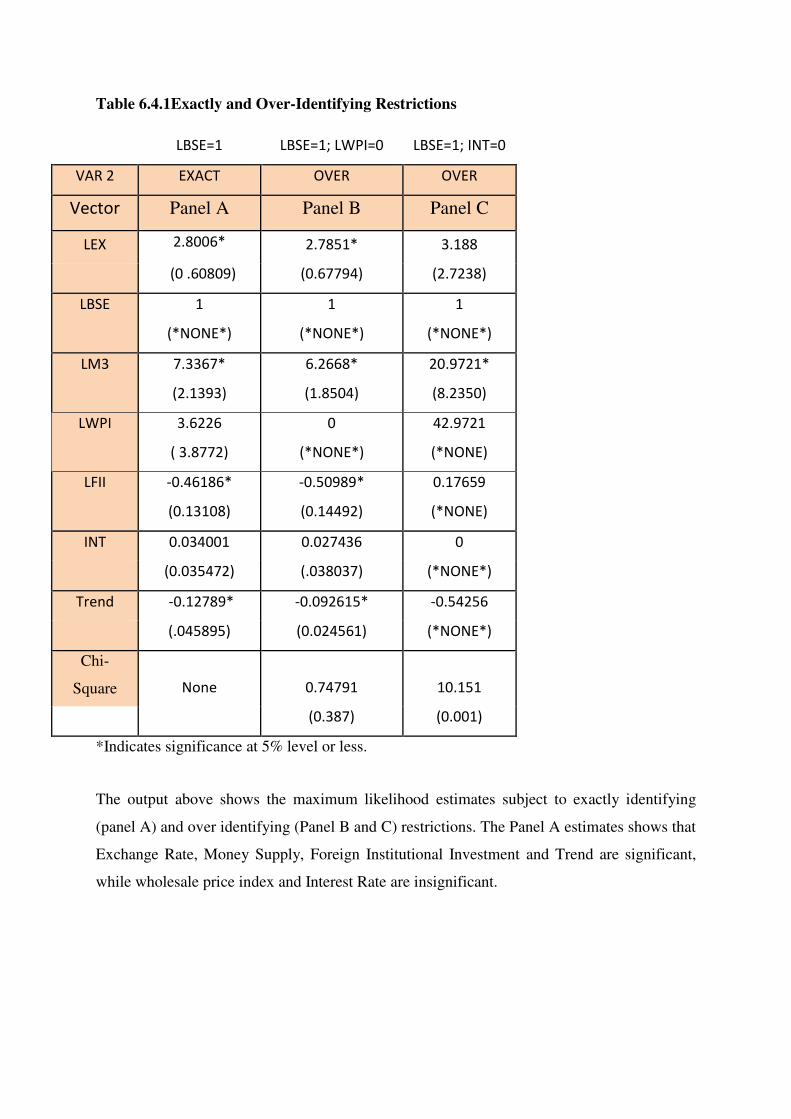
Table 6.4.1Exactly and Over-Identifying Restrictions

LBSE=1 LBSE=1; LWPI=0 LBSE=1; INT=0

VAR 2 EXACT OVER OVER

Vector Panel A Panel B Panel C

LEX 2.8006* 2.7851* 3.188

(0 .60809) (0.67794) (2.7238)

LBSE 1 1 1

(*NONE*) (*NONE*) (*NONE*)

LM3 7.3367* 6.2668* 20.9721*

(2.1393) (1.8504) (8.2350)

LWPI 3.6226 0 42.9721

( 3.8772) (*NONE*) (*NONE)

LFII -0.46186* -0.50989* 0.17659

(0.13108) (0.14492) (*NONE)

INT 0.034001 0.027436 0

(0.035472) (.038037) (*NONE*)

Trend -0.12789* -0.092615* -0.54256

(.045895) (0.024561) (*NONE*)

Chi-

Square None 0.74791 10.151

(0.387) (0.001)

*Indicates significance at 5% level or less.

The output above shows the maximum likelihood estimates subject to exactly identifying

(panel A) and over identifying (Panel B and C) restrictions. The Panel A estimates shows that

Exchange Rate, Money Supply, Foreign Institutional Investment and Trend are significant,

while wholesale price index and Interest Rate are insignificant.

For the above analysis, we arrive at the following co-integrating equation (numbers in

parentheses are standard deviations.

LBSE+0.28006LEX+7.3367LM3-0.46186LFII

(0.60809) (2.1393 ) 0.13108

However, ignoring Wholesale price index and Interest rate would mean going against the

theoretical framework. Moreover, the above mentioned studies and theories strongly support

the existence of Interest Rate and Inflation. Removing these variables statistically, as the

results showed, will be correct; Therefore, this paper will proceed with the model with the

existence of wholesale price index and Interest Rate variables in the long run.

6.5 Vector Error Correction Model (VECM)

Until now, we tested the long run coefficients of the variables against the theoretically

expected values and found out if the variables are statistically significant or not, but the

cointegrated relationship does not talk about causality i.e. which variable is

Leader/independent and which variable is follower/dependent. Information on direction of

Granger-causation can be particularly useful for investors. By knowing which variable is

exogenous (Leader/Independent) and endogenous (Follower/dependent), investors can better

forecast or predict expected results of their investment. Typically, an investor would be

interested to know whether BSE Index, interest rates, money supply or exchange rate is the

exogenous variable, due to the reason that investor would closely monitor the performance

BSE Index or economic indicator as it would have significant impact on the expected

movement of other indexes in which the investor has invested or policy makers are concerned

with. This exogenous or most exogenous variable would be the variable of interest to the

investor.

In line what have been written, the next step of analysis involves the Vector Error Correction

Model (VECM). In this step, in addition to decomposing the change in each variable to short-

term and long-term components, study will be able to ascertain which variables are in fact

exogenous and which are endogenous. The principle in action here is that of Granger-

causality, a form of temporal causality where it is determined the extent to which the change

in one variable is caused by another variable in a previous period.

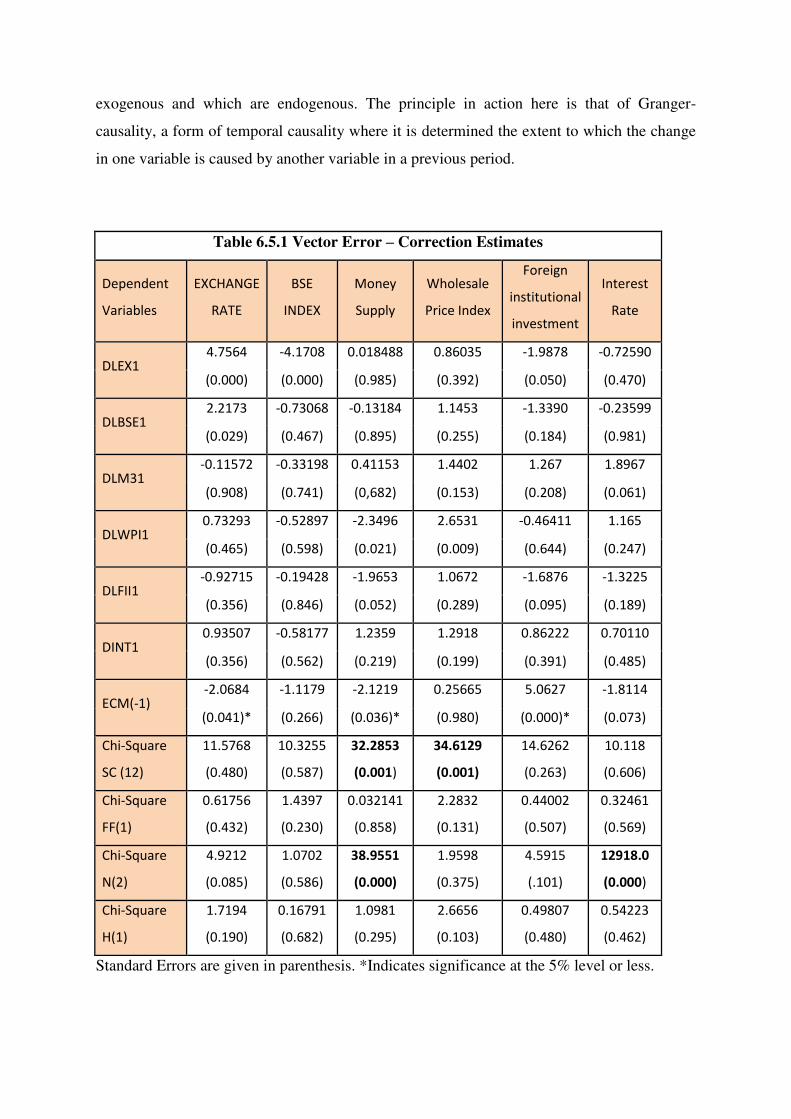
Table 6.5.1 Vector Error – Correction Estimates

Dependent

Variables

EXCHANGE

RATE

BSE

INDEX

Money

Supply

Wholesale

Price Index

Foreign

institutional

investment

Interest

Rate

DLEX1 4.7564 -4.1708 0.018488 0.86035 -1.9878 -0.72590

(0.000) (0.000) (0.985) (0.392) (0.050) (0.470)

DLBSE1 2.2173 -0.73068 -0.13184 1.1453 -1.3390 -0.23599

(0.029) (0.467) (0.895) (0.255) (0.184) (0.981)

DLM31 -0.11572 -0.33198 0.41153 1.4402 1.267 1.8967

(0.908) (0.741) (0,682) (0.153) (0.208) (0.061)

DLWPI1 0.73293 -0.52897 -2.3496 2.6531 -0.46411 1.165

(0.465) (0.598) (0.021) (0.009) (0.644) (0.247)

DLFII1 -0.92715 -0.19428 -1.9653 1.0672 -1.6876 -1.3225

(0.356) (0.846) (0.052) (0.289) (0.095) (0.189)

DINT1 0.93507 -0.58177 1.2359 1.2918 0.86222 0.70110

(0.356) (0.562) (0.219) (0.199) (0.391) (0.485)

ECM(-1) -2.0684 -1.1179 -2.1219 0.25665 5.0627 -1.8114

(0.041)* (0.266) (0.036)* (0.980) (0.000)* (0.073)

Chi-Square

SC (12)

11.5768

(0.480)

10.3255

(0.587)

32.2853

(0.001)

34.6129

(0.001)

14.6262

(0.263)

10.118

(0.606)

Chi-Square

FF(1)

0.61756

(0.432)

1.4397

(0.230)

0.032141

(0.858)

2.2832

(0.131)

0.44002

(0.507)

0.32461

(0.569)

Chi-Square

N(2)

4.9212

(0.085)

1.0702

(0.586)

38.9551

(0.000)

1.9598

(0.375)

4.5915

(.101)

12918.0

(0.000)

Chi-Square

H(1)

1.7194

(0.190)

0.16791

(0.682)

1.0981

(0.295)

2.6656

(0.103)

0.49807

(0.480)

0.54223

(0.462)

Standard Errors are given in parenthesis. *Indicates significance at the 5% level or less.

By examining the error correction term, et-1, for each variable, and checking whether it is

significant, paper found that, as showed in the table above BSE Index, Wholesale Price Index

and Interest rates are exogenous variables, while remaining variables Exchange Rate, Money

Supply and Foreign Institutional Investment are Endogenous variables. The implication of

this result is that, as far as the analysed variables are concerned, the interest of variables for

Investors, policy makers would be BSE Index, Wholesale Price Index and Interest rates.

Policy implication could be focusing on Interest rates (finance variables), Inflation and Stock

Market can help the economy in managing money supply, FII investment and exchange rate

of the country. These variables being the exogenous variables, they would receive the market

shocks and transmit the effect of those shocks to other variables. An investor, who has

invested in BSE, it would be in his interest to keep a track of Interest rate and wholesale price

Index as these two variables have significant effects on BSE.

The diagnostics are chi-squared statistics for serial correlation (SC), functional form (FF),

normality (N), heteroskedaticity (H), indicates that equations are well specified with

exception of Money Supply, Whole sale Price Index and interest rates equations where it can

be observed issues related to functional form, normality and heteroskedaticity. However,

since paper is looking for long term relationship among the variables, the above mentioned

issues will be neglected, so analysis can proceed to the next step.

The diagnostics of all the equations of the error-correction model (testing for the presence of

autocorrelation, functional form, normality, and heteroscedasticity) tend to indicate that the

equations are well specified. We also checked the stability of the coefficients by the CUSUM

and CUSUM SQUARE tests which (Figure 1) indicate that they are stable and according to

the results, there was no structural break during the study period.

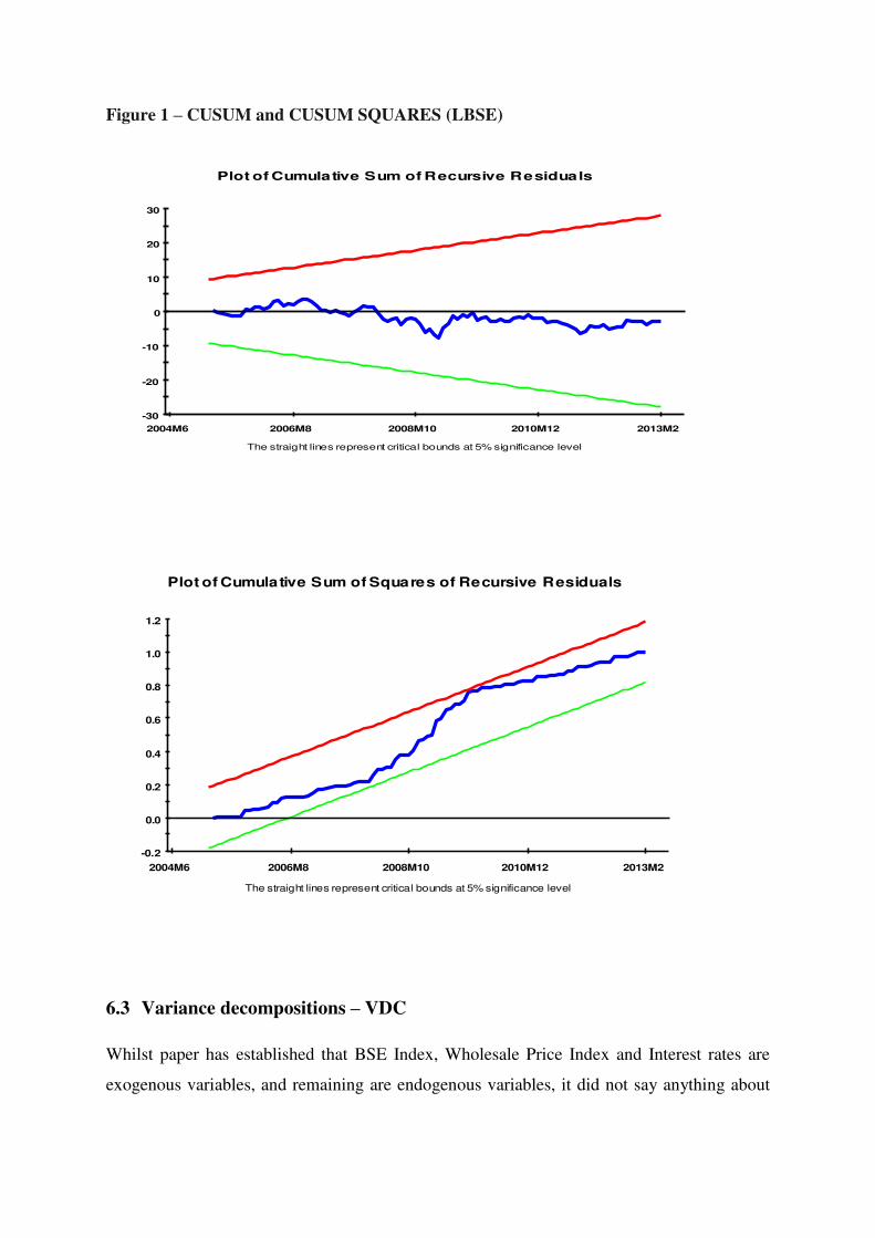
Figure 1 – CUSUM and CUSUM SQUARES (LBSE)

6.3 Variance decompositions – VDC

Whilst paper has established that BSE Index, Wholesale Price Index and Interest rates are

exogenous variables, and remaining are endogenous variables, it did not say anything about

-30

-20

-10

0

10

20

30

2004M6 2006M8 2008M10 2010M12 2013M2

The straight lines represent critical bounds at 5% significance level

Plot of Cumulative Sum of Recursive Residuals

-0.2

0.0

0.2

0.4

0.6

0.8

1.0

1.2

2004M6 2006M8 2008M10 2010M12 2013M2

The straight lines represent critical bounds at 5% significance level

Plot of Cumulative Sum of Squares of Recursive Residuals

the relative endogeneity or exogeneity of variables, In other words, of the remaining

variables, which is the strongest “follower” variable compared to others, or the least

follower? As the VECM is not able to assist us in this regard, paper move to the step six

which is variance decomposition (VDC). Relative endogeneity can be ascertained in the

following way. VDC decomposes the variance of forecast error of each variable into

proportions attributable to shocks from each variable in the system, including its own. The

most endogenous variable is thus the variable whose variation is explained mostly by its own

past variations.

Paper applied generalized and orthogonalized VDCs and obtained the following results.

Although We did apply Orthogonalized VDC, looking at its limitations, as it depends on the

particular ordering of variables in the VAR and assumes that when a particular variable is

shocked, all other variables in the system are switched off, we did not report the results of

Orthogonalized VDC and we went ahead with the Generalized VDC analysis.

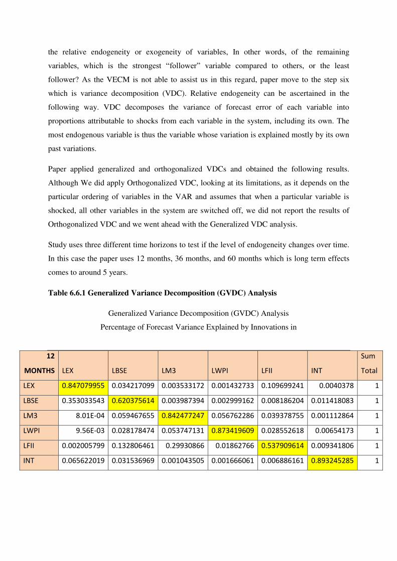
Study uses three different time horizons to test if the level of endogeneity changes over time.

In this case the paper uses 12 months, 36 months, and 60 months which is long term effects

comes to around 5 years.

Table 6.6.1 Generalized Variance Decomposition (GVDC) Analysis

Generalized Variance Decomposition (GVDC) Analysis

Percentage of Forecast Variance Explained by Innovations in

12

MONTHS LEX LBSE LM3 LWPI LFII INT

Sum

Total

LEX 0.847079955 0.034217099 0.003533172 0.001432733 0.109699241 0.0040378 1

LBSE 0.353033543 0.620375614 0.003987394 0.002999162 0.008186204 0.011418083 1

LM3 8.01E-04 0.059467655 0.842477247 0.056762286 0.039378755 0.001112864 1

LWPI 9.56E-03 0.028178474 0.053747131 0.873419609 0.028552618 0.00654173 1

LFII 0.002005799 0.132806461 0.29930866 0.01862766 0.537909614 0.009341806 1

INT 0.065622019 0.031536969 0.001043505 0.001666061 0.006886161 0.893245285 1

36

months LEX LBSE LM3 LWPI LFII INT

Sum

Total

LEX 0.833793641 0.035500216 0.003801028 0.001210004 0.123063026 0.003592147 1

LBSE 0.365024445 0.612884292 0.003604291 0.002433284 0.003942558 0.011780284 1

LME 0.000663616 0.066971593 0.81693787 0.062156915 0.044431857 0.000694869 1

LWPI 0.010528433 0.02755061 0.055661977 0.870533092 0.030802079 0.00715939 1

LFII 0.001386977 0.17229798 0.374663365 0.022325693 0.423263903 0.006394647 1

INT 0.07023373 0.034432786 0.000836151 0.001331898 0.006921133 0.883457164 1

60

Months LEX LBSE LM3 LWPI LFII INT

Sum

Total

LEX 0.830098632 0.035723095 0.003851559 0.001162848 0.125667293 0.003496572 1

LBSE 0.367667041 0.61157059 0.003525907 0.002316286 0.003059409 0.011860768 1

LM3 0.000640519 0.069258508 0.819582509 0.063941277 0.045965521 0.000611666 1

LWPI 0.010698983 0.02734704 0.055906081 0.867598575 0.031181988 0.007267332 1

LFII 0.001218898 0.182915754 0.394912871 0.023318538 0.392040048 0.005593891 1

INT 0.071431135 0.035151446 0.000796231 0.001266812 0.006951859 0.884402517 1

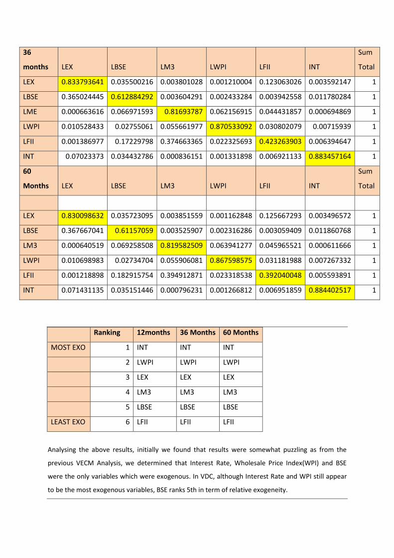
Ranking 12months 36 Months 60 Months

MOST EXO 1 INT INT INT

2 LWPI LWPI LWPI

3 LEX LEX LEX

4 LM3 LM3 LM3

5 LBSE LBSE LBSE

LEAST EXO 6 LFII LFII LFII

Analysing the above results, initially we found that results were somewhat puzzling as from the

previous VECM Analysis, we determined that Interest Rate, Wholesale Price Index(WPI) and BSE

were the only variables which were exogenous. In VDC, although Interest Rate and WPI still appear

to be the most exogenous variables, BSE ranks 5th in term of relative exogeneity.

Interestingly, the ranking of the variables between all time periods i.e 12 months, 36 months and 60

months remains the same. The results show that FII is the least exogenous variable among all. This

confirms the findings of Chandra (2012) who reported that in general, the FIIs seem to be

chasing the Indian stock market returns.

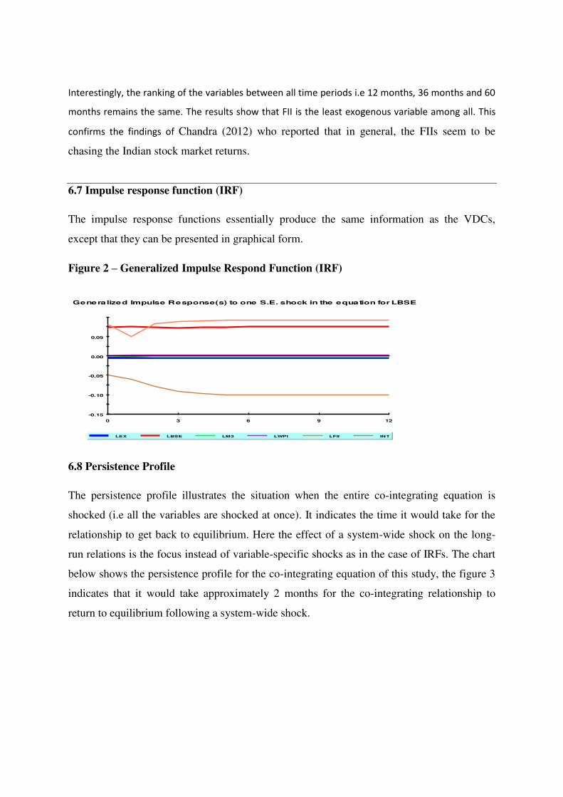
6.7 Impulse response function (IRF)

The impulse response functions essentially produce the same information as the VDCs,

except that they can be presented in graphical form.

Figure 2 – Generalized Impulse Respond Function (IRF)

6.8 Persistence Profile

The persistence profile illustrates the situation when the entire co-integrating equation is

shocked (i.e all the variables are shocked at once). It indicates the time it would take for the

relationship to get back to equilibrium. Here the effect of a system-wide shock on the long-

run relations is the focus instead of variable-specific shocks as in the case of IRFs. The chart

below shows the persistence profile for the co-integrating equation of this study, the figure 3

indicates that it would take approximately 2 months for the co-integrating relationship to

return to equilibrium following a system-wide shock.

-0.15

-0.10

-0.05

0.00

0.05

0 3 6 9 12

Generalized Impulse Response(s) to one S.E. shock in the equation for LBSE

LEX LBSE LM3 LWPI LFII INT

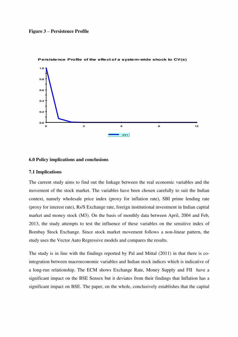
Figure 3 – Persistence Profile

6.0 Policy implications and conclusions

7.1 Implications

The current study aims to find out the linkage between the real economic variables and the

movement of the stock market. The variables have been chosen carefully to suit the Indian

context, namely wholesale price index (proxy for inflation rate), SBI prime lending rate

(proxy for interest rate), Rs/$ Exchange rate, foreign institutional investment in Indian capital

market and money stock (M3). On the basis of monthly data between April, 2004 and Feb,

2013, the study attempts to test the influence of these variables on the sensitive index of

Bombay Stock Exchange. Since stock market movement follows a non-linear pattern, the

study uses the Vector Auto Regressive models and compares the results.

The study is in line with the findings reported by Pal and Mittal (2011) in that there is co-

integration between macroeconomic variables and Indian stock indices which is indicative of

a long-run relationship. The ECM shows Exchange Rate, Money Supply and FII have a

significant impact on the BSE Sensex but it deviates from their findings that Inflation has a

significant impact on BSE. The paper, on the whole, conclusively establishes that the capital

0.0

0.2

0.4

0.6

0.8

1.0

0 3 6 9 12

Persistence Profile of the effect of a system-wide shock to CV(s)

CV1

market indices are dependent on macroeconomic variables even though the same may not be

statistically significant in all the cases.

The study reconfirms the traditional belief that the real economic variables continue to affect

the stock market in the post-reform era in India and also highlights the insignificance of

certain variables with respect to stock market. This has an important implication for the

national policy makers, researchers, corporate managers and regulators.

7.2 Limitations

The study has several limitations that warrant mention to ensure future studies can be built on

this. Among the critical limitation of the study is the lack of sufficient time to digress the

causality between different combinations of the variables. Secondly, the study used monthly

data for about 9 years period. Perhaps a longer period of data could have yielded a more

refined result. Moreover, since it is difficult to find any benchmark interest rate for the entire

time period under study, we have taken the SBI Prime Lending Rate (SBIPLR) as the proxy

for the interest rate (IR) prevailing in the economy. If we had also included Long term Govt

bond rate, Money Market rates might have helped the relevance of the results. Also, apart

from BSE, there are other indices such as, National stock Exchange (NSE) and similar other

indices that might have helped to give better results.

REFERENCES

Abeyratna, G., Pisedtasalasai, A. & Power, D. (2004). Macroeconomic influence on the stock market:

evidence from an emerging market in South Asia. Journal of Emerging Market Finance 3(3): 85-304.

Asprem, M. (1989). Stock Prices Asset Portfolios and Macroeconomic Variables in Ten European

Countries. Journal of Banking and Finance Vo. 13, 589-612.

Bhattacharya, B., & Mukherjee, J. (2002). The nature of the causal relationship between stock market

and macroeconomic aggregates in India: An empirical analysis. In 4th Annual Conference on Money

and Finance, Mumbai.

Bilson, C. M., Brailsford, T. J., & Hooper, V. J. (2001). Selecting macroeconomic variables as

explanatory factors of emerging stock market returns. Pacific-Basin Finance Journal, 9(4), 401-426.

Chandra, A (2012). Cause and effect between FII trading behaviour and stock market returns: The

Indian experience. Journal of Indian Business Research Volume: 4 Issue: 4.

Chen, N. F., Roll, R. & Ross, S. (1986). Economic forces and the stock market. Journal of Business

59(3): 83-403

Hassan, A. H. (2003). Financial integration of stock markets in the Gulf: A multivariate cointegration

analysis. International Journal of Business, Vol. 8, No.3.

Hussin Mohd, at all. (2012). Macroeconomic Variables and Malaysian Islamic Stock Market: A Time

Series Analysis. Journal of Business Studies Quarterly 2012, Vol. 3, No. 4, 1-13.

Ibrahim, M and Aziz, PP. (2003). Macroeconomic Variables and the Malaysian Equity Market: a

View Through Rolling Subsamples”. Journal of Economic Studies, Vol. 30 No. 1, 6-27.

Ibrahim, M and Wan, S.W.Y (2001). Macroeconomic Variables, Exchange Rate and Stock Price: A

Malaysian Perspective. IIUM Journal of Economics and Management, Vol. 9 No. 2, 141-163.

Ibrahim, M. (1999). Macroeconomic Variables and Stock Prices in Malaysia: An Empirical Analysis.

Asian Economic Journal, Vol. 13 No. 2, 219-231.

Ibrahim, M. (2003). Macroeconomic Forces and Capital Market Integration: A VAR Analysis for

Malaysia. Journal of the Asia Pacific Economy, Vol. 8, 19-40.

Lovatt D. & Parikh A. 2000. Stock returns and economic activity: The UK case. European Journal of

Finance 6(3): 280-297.

Maysami, R. C. and Koh, T. S. (2000), A Vector Error Correction Model of the Singapore Stock

Market, International Review of Economics and Finance, 9, 79-156.

Mukherjee, T. K. and Naka, A. (1995), Dynamic Relations between Macroeconomic Variables and

the Japanese Stock Market: An Application of a Vector Error- Correction Model, Journal of Empirical

Research, 18, 223-237.

Pal, K. and Mittal, R.(2011) Impact of macroeconomic indicators on Indian capital markets

Journal of Risk Finance, Volume: 12 Issue: 2.

Pesaran , M. H. and Timmermann, A. (2000), A Recursive Modelling Approach to Predicting U.K.

Stock Returns, Economic Journal , 110, 159-191.

Rashid, A. (2008). Macroeconomic variables and stock market performance: Testing for dynamic

linkages with a known structural break. Savings and Development, 77-102.