remote sensing

Article

Relationship between Spatiotemporal Variations ofClimate, Snow Cover and Plant Phenology over theAlps—An Earth Observation-Based Analysis

Sarah Asam 1,2,* , Mattia Callegari 2, Michael Matiu 3 , Giuseppe Fiore 4,Ludovica De Gregorio 2, Alexander Jacob 2, Annette Menzel 3, Marc Zebisch 2 andClaudia Notarnicola 2

1 German Remote Sensing Data Center (DFD), German Aerospace Center (DLR), 82234 Weßling, Germany2 Institute for Earth Observation, EURAC, Viale Druso 1, 39100 Bolzano, Italy; mattia.callegari@eurac.edu (M.C.);

Ludovica.DeGregorio@eurac.edu (L.D.G.); Alexander.Jacob@eurac.edu (A.J.); Marc.Zebisch@eurac.edu (M.Z.);claudia.notarnicola@eurac.edu (C.N.)

3 Ecoclimatology, Technical University of Munich, 80333 Freising, Germany; michaelmatiu@gmail.com (M.M.);amenzel@wzw.tum.de (A.M.)

4 Dipartimento Interateneo di Fisica “M. Merlin”, Università degli Studi di Bari e Politecnico di Bari,70126 Bari, Italy; gfioreing@gmail.com

* Correspondence: sarah.asam@dlr.de; Tel.: +49-8153281230

Received: 1 September 2018; Accepted: 4 November 2018; Published: 7 November 2018�����������������

Abstract: Alpine ecosystems are particularly sensitive to climate change, and therefore it is ofsignificant interest to understand the relationships between phenology and its seasonal drivers inmountain areas. However, no alpine-wide assessment on the relationship between land surfacephenology (LSP) patterns and its climatic drivers including snow exists. Here, an assessment ofthe influence of snow cover variations on vegetation phenology is presented, which is based ona 17-year time-series of MODIS data. From this data snow cover duration (SCD) and phenologymetrics based on the Normalized Difference Vegetation Index (NDVI) have been extracted at 250 mresolution for the entire European Alps. The combined influence of additional climate drivers onphenology are shown on a regional scale for the Italian province of South Tyrol using reanalyzedclimate data. The relationship between vegetation and snow metrics strongly depended on altitude.Temporal trends towards an earlier onset of vegetation growth, increasing monthly mean NDVI inspring and late summer, as well as shorter SCD were observed, but they were mostly non-significantand the magnitude of these tendencies differed by altitude. Significant negative correlations betweenmonthly mean NDVI and SCD were observed for 15–55% of all vegetated pixels, especially fromDecember to April and in altitudes from 1000–2000 m. On the regional scale of South Tyrol,the seasonality of NDVI and SCD achieved the highest share of correlating pixels above 1500 m,while at lower elevations mean temperature correlated best. Examining the combined effect of climatevariables, for average altitude and exposition, SCD had the highest effect on NDVI, followed by meantemperature and radiation. The presented analysis allows to assess the spatiotemporal patterns ofearth-observation based snow and vegetation metrics over the Alps, as well as to understand therelative importance of snow as phenological driver with respect to other climate variables.

Keywords: mountains; phenology; NDVI; snow cover; climate variability; impact of climate change;MODIS; Alps

Remote Sens. 2018, 10, 1757; doi:10.3390/rs10111757 www.mdpi.com/journal/remotesensing

Remote Sens. 2018, 10, 1757 2 of 26

1. Introduction

Phenology, the science of the timing of annual recurring biological events, has been studiedfor centuries. Within the field of vegetation phenology, these events comprise plant stages such asbud-burst, flowering, leaf unfolding, or leaf-fall. Monitoring and understanding plant phenology isimportant in the context of global change, because the timing and magnitude of phenological events arestrongly sensitive to seasonal and inter-annual climate variability [1–3]. A key aspect of phenologicalstudies is thus determining causal relationships between physiological plant phenomena and theirseasonal and long-term drivers.

Phenological ground networks provide the longest sources of observations, which are oftenspecies specific, detailed, and highly accurate, but at the same time only conclusive for one organismat a certain location [4–8]. To derive spatially exhaustive information, satellite remote sensing data thattrace seasonal changes in the spectral signature of vegetation photosynthetic activity have increasinglybeen used during the last decade [9,10]. Such remote sensing-based analyses are referred to asland surface phenology (LSP) [11–18]. LSP observations provide a spatially integrative view ofcontinuous biophysical canopy properties at coarse scales instead of plant-specific phenological stages.Nevertheless, LSP metrics proofed to be comparable to these development stages, good measures ofphenophases at the ecosystem level, and a suitable proxy indicator of climate variations [19,20].

Due to this sensitivity to climate variability, phenology has gained importance as an indicatorfor ecological responses to climate change [4,21–25]. Concurrently, phenology provides feedbacks toclimate by influencing albedo, temperature and precipitation patterns [26–29]. A reliable representationof vegetation phenology in climate models is therefore necessary to model carbon, energy, and watercycles on a regional to global scale [27,30–32]. In this context, prognostic phenology models have beendeveloped to simulate phenological events based on driving factors such as temperatures, photoperiod,precipitation, or soil moisture [33–42].

Mountain ecosystems are assumed particularly affected by climate change with various effects onecosystems, cryosphere, and hydrological regimes [43–50]. Observed effects of climate warming onmountain phenology are e.g., longer growing seasons [19], the migration of plant species to higheraltitudes [51–54] and the associated impacts on niches and endemic species [53–58]. These changes arelikely to have considerable implications for mountain ecosystem compositing, functioning, and services.The mapping of patterns of alpine phenology and the understanding of the underlying processes onlarge spatial scales is therefore of importance. Further, according to the space-for-time substitutionassumption, the understanding of altitudinal patterns of phenology is useful to estimate futurephenological behavior [59].

However, few LSP studies have focused on alpine environments, and in consequence,the processes and changes of mountain phenology are insufficiently investigated. Only in recent years,mountains have begun attracting more attention within the LSP literature, with some studies located inthe European Alps. Studer et al. [20] compared in situ observed spring phases with LSP metrics derivedfrom Advanced Very High-Resolution Radiometer (AVHRR) data in Switzerland between 1982 and2001 and showed their sensitivity to temperature. Also, Fontana et al. [60] focused on the Swiss Alps,analyzing grassland phenology from 2001 to 2005 using AVHRR, SPOT (Satellite Pour l’Observationde la Terre)) VEGETATION, and MODIS (Moderate Resolution Imaging Spectroradiometer) Terra data.The phenological patterns of alpine larch forests and grasslands in the Aosta Valley of northwesternItaly have been studied by Busetto et al. [61] and Colombo et al. [62,63] using MODIS time seriesfor different periods between 2000 to 2009 in relation to climatic factors and elevation. Choler [64]presented a study on grassland phenology in the French Alps, in which plant responses to snow coverduration are analyzed. However, there are only few studies covering the entire Alps. As part of acontinental study in which they analyzed AVHRR time series over the period of 1982–2001, Stöckli andVidale [19] observed for the Alps inter-annual and seasonal variations as well as broad patterns relatedto topography, but they did not provide information on variabilities within the Alps. Also on an

Remote Sens. 2018, 10, 1757 3 of 26

alpine-wide scale, Jolly et al. [65] and Reichstein et al. [66] analyzed the responses of low and highelevation phenology to the 2003 heat wave in the Alps.

The knowledge on LSP patterns and trends over the Alps is hence scattered and limited to specificareas and land cover types. In addition, the available regional studies rely on coarse remote sensingdata of 1–8 km spatial resolution. Considering that mountains are heterogeneous landscapes withstrongly varying altitudinal gradients and microclimatic conditions, this might reduce the reliability ofthese analyses [67]. Fisher et al. [10] report that small-scale topographical differences in the order of50 m can result in a 1–2 week difference in the start of season (SOS), and Inouye and Wielgolaski [68] aswell as Kulonen et al. [69] stress the relevance of microhabitat differences. This highlights the necessityof using the highest spatial resolution data available for spatially explicit analyses.

Moreover, no alpine-wide assessment on the relationship between LSP patterns and its climaticdrivers exist to date. In this context, an often neglected but very important driver of alpine phenologyis snow. Many studies [62,64,68,70–72] stress the relevance of snow cover and snowmelt for mountainphenology. The relationship between snow seasonality and phenology is however hardly assessedover large scales and on a per-pixel basis [72]. In a study on the Tibetan Plateau [73], mean NormalizedDifference Vegetation Index (NDVI) and snow cover duration (SCD) metrics have been correlatedfor some individual and accumulated months over ten years, but not looking into the strength of theidentified correlations. Xie et al. [74] correlated inter-annual changes of phenological metrics to snowaccumulation and melt date, but they conducted this analysis only for the Swiss Alps.

This paper aims at closing these gaps by presenting 17-year time-series of snow cover andphenology for the entire European Alps, using the highest possible spatial resolution of the MODISland surface reflectance data (250 m). The main objective is to show the potential of the joint analysisof earth observation-based vegetation productivity measures and snow metrics, aimed at answeringthe following questions:

i Which patterns show the temporal and spatial variabilities of snow and vegetation phenology independency of topography and land cover over the Alps?

ii Can statistical relationships between vegetation phenology and snow cover be detected independency of the altitude? Are there time lags?

iii What is the common seasonality between vegetation phenology, snow, and climate parameters?Which parameters are most important in which altitude? Are there time lags?

iv Is there a combined influence of climate parameters and snow on phenology?

The above-mentioned data sets are used to answer the research questions (i) and (ii) at anunprecedented temporal and spatial resolution (up to 250 m) and extent (the entire Alps for the years2000–2017). Since a comprehensive set of climate observations was only available for the Italianprovince of South Tyrol, the influence of different climate parameters [questions (iii) and (iv)] wastested for this area.

2. Materials and Methods

2.1. Study Area

The study area includes the Alpine range (43.0◦–48.6◦N/4.2◦–17.1◦E). The Alps as defined by theAlpine Convention (green shape in Figure 1) cover an area of 191,000 km2, stretching across 1200 kmand eight states: Austria, France, Germany, Italy, Liechtenstein, Monaco, Slovenia, and Switzerland.Its maximum width is 300 km, between Bavaria and Northern Italy. The Alps are the highest and mostextensive mountain range that entirely lies in Europe. The height distribution decreases from west toeast with the lowest altitudes being the Mediterranean Sea level and Mont Blanc being the highestpeak of the Alps (4810 m).

The climate in the Alps has a very distinct spatial pattern, with temperature tracing altitude andshowing a general increasing gradient from north to south and from east to west. Precipitation is

Remote Sens. 2018, 10, 1757 4 of 26

highest along the outer chains and more abundant on the northern slopes and at higher altitudes.The rainiest areas are the Jura Mountains, Bernese Alps, Lepontine Alps, Bavarian Alps and the JulianAlps, where precipitation exceeds 2000 mm per year [75]. The zones characterized by low rainfall arethose in correspondence of the great longitudinal valleys such as the upper Rhône valley, the DoraBaltea valley, the Valtellina Valley, the Venosta Valley, and the Engadin. Here, annual precipitation isgenerally below 800 mm per year [75,76]. On smaller scales, the climate is highly related to topography,as altitude and exposure to sunlight and wind influence the individual slopes.

Remote Sens. 2018, 10, x FOR PEER REVIEW    4 of 27 

is  generally  below  800 mm  per  year  [75,76]. On  smaller  scales,  the  climate  is  highly  related  to 

topography, as altitude and exposure to sunlight and wind influence the individual slopes. 

 

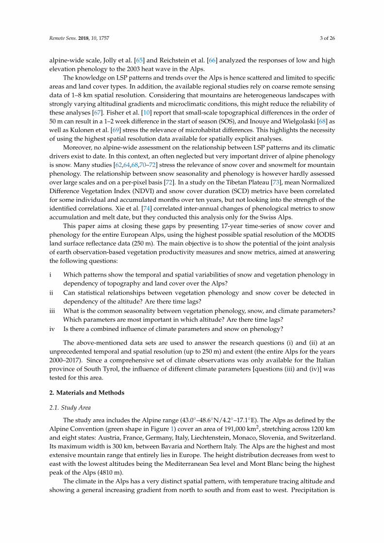
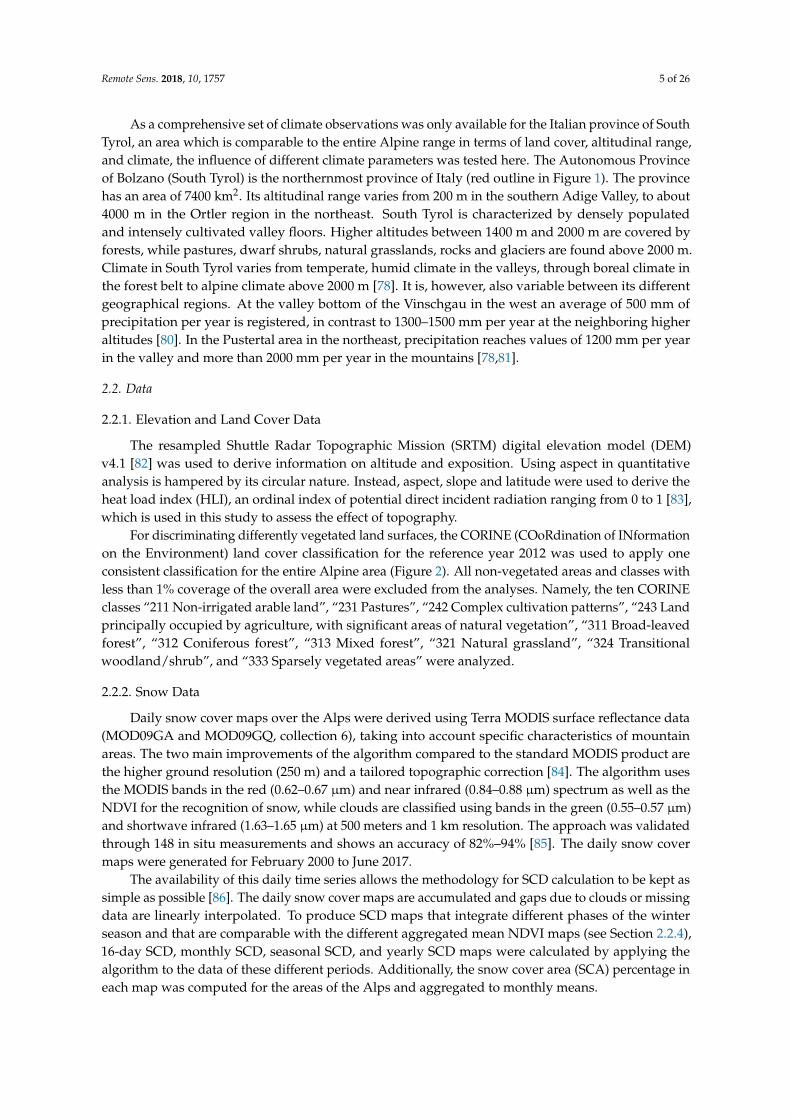
Figure 1. Overview of the study area showing the elevation with the boundary of the Alps as defined 

by the Alpine Convention (green), state borders (white), and the border of the province of Bolzano 

(South Tyrol, red). 

Almost half of  the Alpine area  (43%)  is  covered by  forests  [77].  In  the north  and  the  south, 

deciduous trees dominate the lower slopes, while the upper areas are mostly covered by evergreen 

forests. Conifers abound  in  the dry and high altitudes and  in  the  inland areas. Agricultural areas 

cover almost 40% of the alpine area, of which meadows and mountain pastures make up 18% [78]. 

Mostly occurring in the highest altitudes, about 10% of the alpine areas are glaciers and perpetual 

snow, sparsely vegetated or bare areas. Urban areas, which make up about 5% of the area, are the 

living environment for 14 million people [79] (Figure 2). 

 

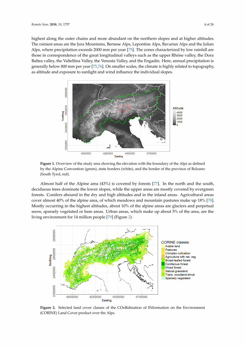
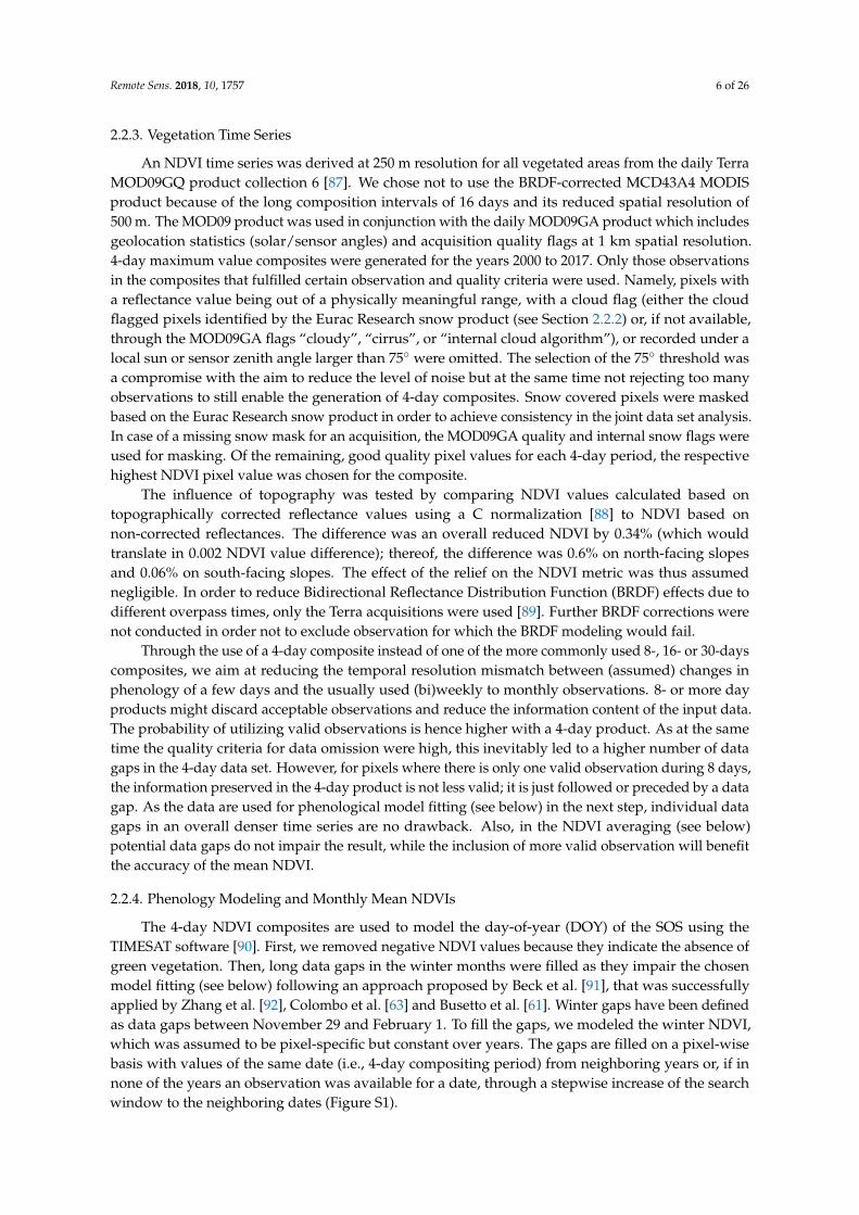
Figure  2.  Selected  land  cover  classes  of  the  COoRdination  of  INformation  on  the  Environment 

(CORINE) Land Cover product over the Alps. 

As a comprehensive set of climate observations was only available for the Italian province of 

South Tyrol, an area which is comparable to the entire Alpine range in terms of land cover, altitudinal 

range, and climate, the influence of different climate parameters was tested here. The Autonomous 

Province of Bolzano (South Tyrol) is the northernmost province of Italy (red outline in Figure 1). The 

province has an area of 7400 km2. Its altitudinal range varies from 200 m in the southern Adige Valley, 

Figure 1. Overview of the study area showing the elevation with the boundary of the Alps as definedby the Alpine Convention (green), state borders (white), and the border of the province of Bolzano(South Tyrol, red).

Almost half of the Alpine area (43%) is covered by forests [77]. In the north and the south,deciduous trees dominate the lower slopes, while the upper areas are mostly covered by evergreenforests. Conifers abound in the dry and high altitudes and in the inland areas. Agricultural areascover almost 40% of the alpine area, of which meadows and mountain pastures make up 18% [78].Mostly occurring in the highest altitudes, about 10% of the alpine areas are glaciers and perpetualsnow, sparsely vegetated or bare areas. Urban areas, which make up about 5% of the area, are theliving environment for 14 million people [79] (Figure 2).

Remote Sens. 2018, 10, x FOR PEER REVIEW    4 of 27 

is  generally  below  800 mm  per  year  [75,76]. On  smaller  scales,  the  climate  is  highly  related  to 

topography, as altitude and exposure to sunlight and wind influence the individual slopes. 

 

Figure 1. Overview of the study area showing the elevation with the boundary of the Alps as defined 

by the Alpine Convention (green), state borders (white), and the border of the province of Bolzano 

(South Tyrol, red). 

Almost half of  the Alpine area  (43%)  is  covered by  forests  [77].  In  the north  and  the  south, 

deciduous trees dominate the lower slopes, while the upper areas are mostly covered by evergreen 

forests. Conifers abound  in  the dry and high altitudes and  in  the  inland areas. Agricultural areas 

cover almost 40% of the alpine area, of which meadows and mountain pastures make up 18% [78]. 

Mostly occurring in the highest altitudes, about 10% of the alpine areas are glaciers and perpetual 

snow, sparsely vegetated or bare areas. Urban areas, which make up about 5% of the area, are the 

living environment for 14 million people [79] (Figure 2). 

 

Figure  2.  Selected  land  cover  classes  of  the  COoRdination  of  INformation  on  the  Environment 

(CORINE) Land Cover product over the Alps. 

As a comprehensive set of climate observations was only available for the Italian province of 

South Tyrol, an area which is comparable to the entire Alpine range in terms of land cover, altitudinal 

range, and climate, the influence of different climate parameters was tested here. The Autonomous 

Province of Bolzano (South Tyrol) is the northernmost province of Italy (red outline in Figure 1). The 

province has an area of 7400 km2. Its altitudinal range varies from 200 m in the southern Adige Valley, 

Figure 2. Selected land cover classes of the COoRdination of INformation on the Environment(CORINE) Land Cover product over the Alps.

Remote Sens. 2018, 10, 1757 5 of 26

As a comprehensive set of climate observations was only available for the Italian province of SouthTyrol, an area which is comparable to the entire Alpine range in terms of land cover, altitudinal range,and climate, the influence of different climate parameters was tested here. The Autonomous Provinceof Bolzano (South Tyrol) is the northernmost province of Italy (red outline in Figure 1). The provincehas an area of 7400 km2. Its altitudinal range varies from 200 m in the southern Adige Valley, to about4000 m in the Ortler region in the northeast. South Tyrol is characterized by densely populatedand intensely cultivated valley floors. Higher altitudes between 1400 m and 2000 m are covered byforests, while pastures, dwarf shrubs, natural grasslands, rocks and glaciers are found above 2000 m.Climate in South Tyrol varies from temperate, humid climate in the valleys, through boreal climate inthe forest belt to alpine climate above 2000 m [78]. It is, however, also variable between its differentgeographical regions. At the valley bottom of the Vinschgau in the west an average of 500 mm ofprecipitation per year is registered, in contrast to 1300–1500 mm per year at the neighboring higheraltitudes [80]. In the Pustertal area in the northeast, precipitation reaches values of 1200 mm per yearin the valley and more than 2000 mm per year in the mountains [78,81].

2.2. Data

2.2.1. Elevation and Land Cover Data

The resampled Shuttle Radar Topographic Mission (SRTM) digital elevation model (DEM)v4.1 [82] was used to derive information on altitude and exposition. Using aspect in quantitativeanalysis is hampered by its circular nature. Instead, aspect, slope and latitude were used to derive theheat load index (HLI), an ordinal index of potential direct incident radiation ranging from 0 to 1 [83],which is used in this study to assess the effect of topography.

For discriminating differently vegetated land surfaces, the CORINE (COoRdination of INformationon the Environment) land cover classification for the reference year 2012 was used to apply oneconsistent classification for the entire Alpine area (Figure 2). All non-vegetated areas and classes withless than 1% coverage of the overall area were excluded from the analyses. Namely, the ten CORINEclasses “211 Non-irrigated arable land”, “231 Pastures”, “242 Complex cultivation patterns”, “243 Landprincipally occupied by agriculture, with significant areas of natural vegetation”, “311 Broad-leavedforest”, “312 Coniferous forest”, “313 Mixed forest”, “321 Natural grassland”, “324 Transitionalwoodland/shrub”, and “333 Sparsely vegetated areas” were analyzed.

2.2.2. Snow Data

Daily snow cover maps over the Alps were derived using Terra MODIS surface reflectance data(MOD09GA and MOD09GQ, collection 6), taking into account specific characteristics of mountainareas. The two main improvements of the algorithm compared to the standard MODIS product arethe higher ground resolution (250 m) and a tailored topographic correction [84]. The algorithm usesthe MODIS bands in the red (0.62–0.67 µm) and near infrared (0.84–0.88 µm) spectrum as well as theNDVI for the recognition of snow, while clouds are classified using bands in the green (0.55–0.57 µm)and shortwave infrared (1.63–1.65 µm) at 500 meters and 1 km resolution. The approach was validatedthrough 148 in situ measurements and shows an accuracy of 82%–94% [85]. The daily snow covermaps were generated for February 2000 to June 2017.

The availability of this daily time series allows the methodology for SCD calculation to be kept assimple as possible [86]. The daily snow cover maps are accumulated and gaps due to clouds or missingdata are linearly interpolated. To produce SCD maps that integrate different phases of the winterseason and that are comparable with the different aggregated mean NDVI maps (see Section 2.2.4),16-day SCD, monthly SCD, seasonal SCD, and yearly SCD maps were calculated by applying thealgorithm to the data of these different periods. Additionally, the snow cover area (SCA) percentage ineach map was computed for the areas of the Alps and aggregated to monthly means.

Remote Sens. 2018, 10, 1757 6 of 26

2.2.3. Vegetation Time Series

An NDVI time series was derived at 250 m resolution for all vegetated areas from the daily TerraMOD09GQ product collection 6 [87]. We chose not to use the BRDF-corrected MCD43A4 MODISproduct because of the long composition intervals of 16 days and its reduced spatial resolution of500 m. The MOD09 product was used in conjunction with the daily MOD09GA product which includesgeolocation statistics (solar/sensor angles) and acquisition quality flags at 1 km spatial resolution.4-day maximum value composites were generated for the years 2000 to 2017. Only those observationsin the composites that fulfilled certain observation and quality criteria were used. Namely, pixels witha reflectance value being out of a physically meaningful range, with a cloud flag (either the cloudflagged pixels identified by the Eurac Research snow product (see Section 2.2.2) or, if not available,through the MOD09GA flags “cloudy”, “cirrus”, or “internal cloud algorithm”), or recorded under alocal sun or sensor zenith angle larger than 75◦ were omitted. The selection of the 75◦ threshold wasa compromise with the aim to reduce the level of noise but at the same time not rejecting too manyobservations to still enable the generation of 4-day composites. Snow covered pixels were maskedbased on the Eurac Research snow product in order to achieve consistency in the joint data set analysis.In case of a missing snow mask for an acquisition, the MOD09GA quality and internal snow flags wereused for masking. Of the remaining, good quality pixel values for each 4-day period, the respectivehighest NDVI pixel value was chosen for the composite.

The influence of topography was tested by comparing NDVI values calculated based ontopographically corrected reflectance values using a C normalization [88] to NDVI based onnon-corrected reflectances. The difference was an overall reduced NDVI by 0.34% (which wouldtranslate in 0.002 NDVI value difference); thereof, the difference was 0.6% on north-facing slopesand 0.06% on south-facing slopes. The effect of the relief on the NDVI metric was thus assumednegligible. In order to reduce Bidirectional Reflectance Distribution Function (BRDF) effects due todifferent overpass times, only the Terra acquisitions were used [89]. Further BRDF corrections werenot conducted in order not to exclude observation for which the BRDF modeling would fail.

Through the use of a 4-day composite instead of one of the more commonly used 8-, 16- or 30-dayscomposites, we aim at reducing the temporal resolution mismatch between (assumed) changes inphenology of a few days and the usually used (bi)weekly to monthly observations. 8- or more dayproducts might discard acceptable observations and reduce the information content of the input data.The probability of utilizing valid observations is hence higher with a 4-day product. As at the sametime the quality criteria for data omission were high, this inevitably led to a higher number of datagaps in the 4-day data set. However, for pixels where there is only one valid observation during 8 days,the information preserved in the 4-day product is not less valid; it is just followed or preceded by a datagap. As the data are used for phenological model fitting (see below) in the next step, individual datagaps in an overall denser time series are no drawback. Also, in the NDVI averaging (see below)potential data gaps do not impair the result, while the inclusion of more valid observation will benefitthe accuracy of the mean NDVI.

2.2.4. Phenology Modeling and Monthly Mean NDVIs

The 4-day NDVI composites are used to model the day-of-year (DOY) of the SOS using theTIMESAT software [90]. First, we removed negative NDVI values because they indicate the absence ofgreen vegetation. Then, long data gaps in the winter months were filled as they impair the chosenmodel fitting (see below) following an approach proposed by Beck et al. [91], that was successfullyapplied by Zhang et al. [92], Colombo et al. [63] and Busetto et al. [61]. Winter gaps have been definedas data gaps between November 29 and February 1. To fill the gaps, we modeled the winter NDVI,which was assumed to be pixel-specific but constant over years. The gaps are filled on a pixel-wisebasis with values of the same date (i.e., 4-day compositing period) from neighboring years or, if innone of the years an observation was available for a date, through a stepwise increase of the searchwindow to the neighboring dates (Figure S1).

Remote Sens. 2018, 10, 1757 7 of 26

Similar to vegetation in high-latitude environments [91], modeling the annual vegetation growthof high-altitude environments faces special challenges such as rather short vegetation periods dueto the above described long winter gaps, and steep increases and decreases of the NDVI signal inspring and autumn. Beck et al. [91] showed that a double logistic function is an appropriate method todescribe NDVI in such biomes, if the winter NDVI is provided as one of the six model parameters.Hence, in conjunction with applying a median filter (Spike value = 0.5) for outlier removal, a doublelogistic fitting method (2–3 envelope iterations and adaptation strength 3–8, depending on land cover)was applied in the TIMESAT software. In a last step, a 0.5 amplitude threshold was selected to estimateSOS, in order to cover different characteristics of ground phenology [93]. As one aim of the study is theassessment of relative changes in SOS, we assumed that the choice of threshold will not influence theresult as long as the same method is applied to all data sets. The maps have been filtered by removingpixels with a SOS before DOY 30 (30 January) and after DOY 212 (31 July).

In addition to the SOS metric, NDVI time series have the potential to track the temporaldevelopment of vegetation activity continuously throughout the vegetation period. Therefore, 16-dayand monthly mean NDVI maps were calculated based on the 4-day composites in addition to the SOS,in order to trace the temporal development of vegetation over the year and to correlate it with thetemporally highly variable snow cover data (see Section 2.3).

As stated by many authors working in northern latitudes [19,20,94–99], detecting vegetationgreen-up from remote sensing-based vegetation indices (VIs) is difficult in areas affected by snow,as snow acts as a confounding factor in LSP. Changes in vegetative phenophases, i.e., the green-updue to the emergence of leaves, have a similar influence on the reflectance in the red and near-infraredspectral domain as has the melting of snow, i.e., an increase in the NDVI value [100]. Due to the stronglinkage of both processes with temperature increase, snowmelt and vegetation green-up can occurvery closely in time, rendering the distinction of both processes a challenging task. Some studieshave suggested the use of other VIs in order to overcome this issue [11,12,94,97,99,101]. These VIs relyhowever always on additional spectral information or input data, which is available in the MODISdata only at reduced spatial resolution. In order to account for the above mentioned high spatialheterogeneity of the alpine environment, it was therefore decided to rely on the NDVI time seriesand to apply the Eurac MODIS snow product for masking snow-influenced observations instead.Through the masking of snow-covered pixels, low NDVI values are removed from the time series. Theremaining minimum NDVI of a pixel is hence related to the vegetation minimum (“winter NDVI”)and an increase in NDVI from this minimum is not related to a decrease in snow coverage, butreflects changes of the vegetation canopy. In combination with the above-mentioned gap-filling andthresholding approaches, this ensures that snow melt is not affecting SOS estimation.

2.2.5. Climate Data

Hourly climate data (temperature, precipitation, radiation, relative humidity, wind, air pressure)were available on a 2 km by 2 km grid for the period 2004–2013 in the region of South Tyrol. The WeatherResearch and Forecasting (WRF) model reanalysis data were provided by the meteorological servicecompany CISMA (www.cisma.it). Besides, day length was derived using latitude and date. All valueswere aggregated to 16-day means or sums to reduce the influence of noise. Mean temperature wascalculated as the average of minimum and maximum temperature. Outlier checks were performedbased on which temperature data from June 2005 had to be discarded because of anomalous low values.

2.3. Statistical Analysis

2.3.1. Analysis on Altitudinal and Temporal Variability of Vegetation Metrics and Snow Cover

In order to assess and quantify alpine-wide spatiotemporal patterns and trends in mountainvegetation phenology (SOS and monthly mean NDVI) and snow cover (SCD and SCA), graphs anddescriptive statistics (median and standard deviation) were derived from the MODIS data sets.

Remote Sens. 2018, 10, 1757 8 of 26

Since different phenological patterns and processes are assumed in different biomes and underdifferent topographic site conditions, individual analyses were done for a range of land cover types(see Section 2.2.1), aspects (i.e., HLI zones) and altitudinal zones in the Alps. The HLI data was split infour classes according to the data sets’ quartiles (which are at 0.62, 0.71, 0.82, and 1.0 HLI in the studyregion) and assessed in 100 m steps between 100 m and 3000 m of altitude. Changes in phenology andsnow cover over the years 2001–2017 were tested through the calculation of linear trends.

2.3.2. Pixel-Wise Correlations between NDVI and SCD

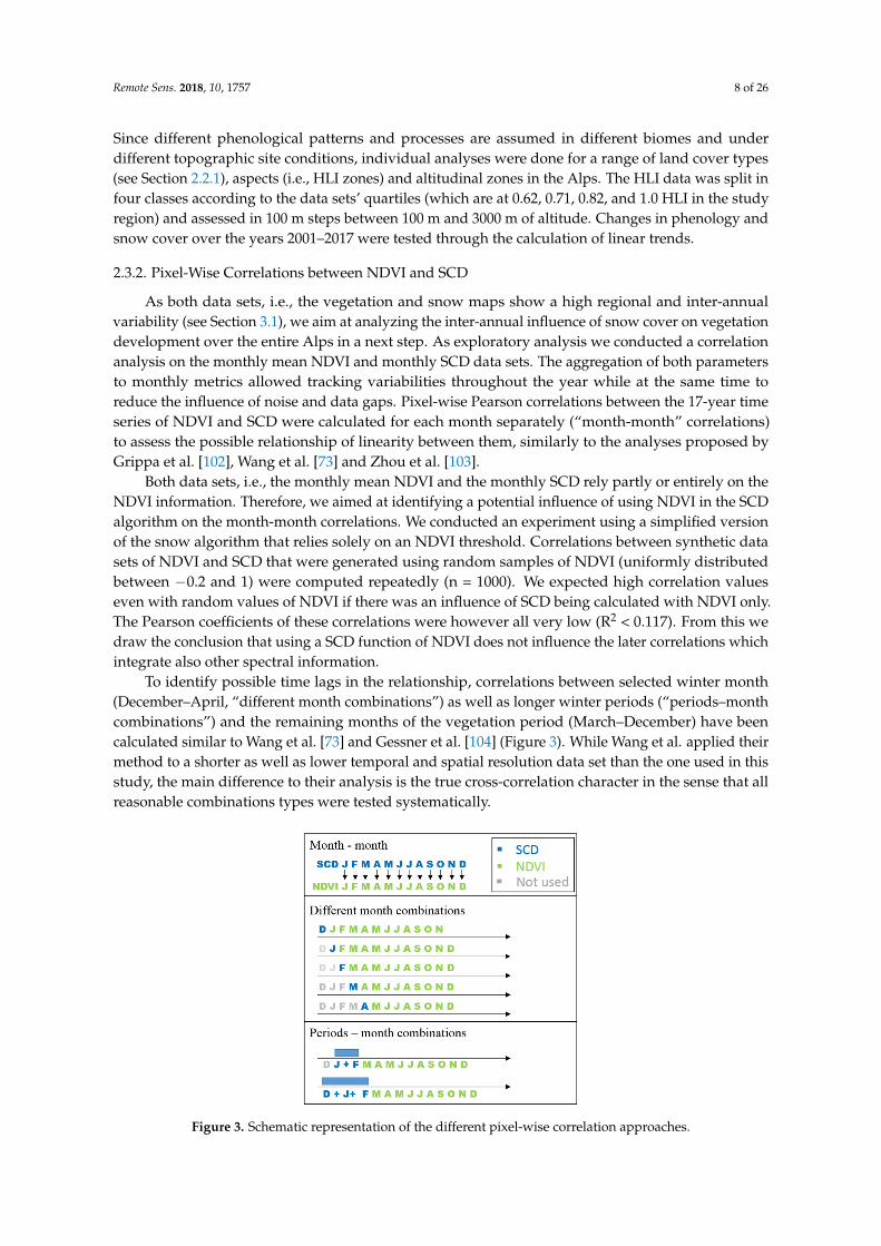
As both data sets, i.e., the vegetation and snow maps show a high regional and inter-annualvariability (see Section 3.1), we aim at analyzing the inter-annual influence of snow cover on vegetationdevelopment over the entire Alps in a next step. As exploratory analysis we conducted a correlationanalysis on the monthly mean NDVI and monthly SCD data sets. The aggregation of both parametersto monthly metrics allowed tracking variabilities throughout the year while at the same time toreduce the influence of noise and data gaps. Pixel-wise Pearson correlations between the 17-year timeseries of NDVI and SCD were calculated for each month separately (“month-month” correlations)to assess the possible relationship of linearity between them, similarly to the analyses proposed byGrippa et al. [102], Wang et al. [73] and Zhou et al. [103].

Both data sets, i.e., the monthly mean NDVI and the monthly SCD rely partly or entirely on theNDVI information. Therefore, we aimed at identifying a potential influence of using NDVI in the SCDalgorithm on the month-month correlations. We conducted an experiment using a simplified versionof the snow algorithm that relies solely on an NDVI threshold. Correlations between synthetic datasets of NDVI and SCD that were generated using random samples of NDVI (uniformly distributedbetween −0.2 and 1) were computed repeatedly (n = 1000). We expected high correlation valueseven with random values of NDVI if there was an influence of SCD being calculated with NDVI only.The Pearson coefficients of these correlations were however all very low (R2 < 0.117). From this wedraw the conclusion that using a SCD function of NDVI does not influence the later correlations whichintegrate also other spectral information.

To identify possible time lags in the relationship, correlations between selected winter month(December–April, “different month combinations”) as well as longer winter periods (“periods–monthcombinations”) and the remaining months of the vegetation period (March–December) have beencalculated similar to Wang et al. [73] and Gessner et al. [104] (Figure 3). While Wang et al. applied theirmethod to a shorter as well as lower temporal and spatial resolution data set than the one used in thisstudy, the main difference to their analysis is the true cross-correlation character in the sense that allreasonable combinations types were tested systematically.

Remote Sens. 2018, 10, x FOR PEER REVIEW    8 of 27 

vegetation development over the entire Alps in a next step. As exploratory analysis we conducted a 

correlation analysis on the monthly mean NDVI and monthly SCD data sets. The aggregation of both 

parameters to monthly metrics allowed tracking variabilities throughout the year while at the same 

time to reduce the influence of noise and data gaps. Pixel‐wise Pearson correlations between the 17‐

year  time  series  of NDVI  and  SCD were  calculated  for  each month  separately  (“month‐month” 

correlations) to assess the possible relationship of linearity between them, similarly to the analyses 

proposed by Grippa et al. [102], Wang et al. [73] and Zhou et al. [103].   

Both data sets, i.e., the monthly mean NDVI and the monthly SCD rely partly or entirely on the 

NDVI  information. Therefore, we aimed at  identifying a potential  influence of using NDVI  in  the 

SCD algorithm on the month‐month correlations. We conducted an experiment using a simplified 

version of the snow algorithm that relies solely on an NDVI threshold. Correlations between synthetic 

data  sets  of  NDVI  and  SCD  that  were  generated  using  random  samples  of  NDVI  (uniformly 

distributed between −0.2 and 1) were computed repeatedly (n = 1000). We expected high correlation 

values even with random values of NDVI  if  there was an  influence of SCD being calculated with 

NDVI only. The Pearson coefficients of  these correlations were however all very  low  (R2 < 0.117). 

From this we draw the conclusion that using a SCD function of NDVI does not influence the later 

correlations which integrate also other spectral information. 

To identify possible time lags in the relationship, correlations between selected winter month 

(December–April,  “different month  combinations”)  as well  as  longer winter  periods  (“periods–

month combinations”) and the remaining months of the vegetation period (March–December) have 

been  calculated  similar  to Wang et al.  [73] and Gessner et al.  [104]  (Figure 3). While Wang et al. 

applied their method to a shorter as well as lower temporal and spatial resolution data set than the 

one used in this study, the main difference to their analysis is the true cross‐correlation character in 

the sense that all reasonable combinations types were tested systematically.   

Pixels with a SCD of “0”, pixels for which less than three observations were available within the 

17‐years vector, and pixels with a standard deviation of zero were excluded  from  the correlation 

analyses. The t‐test was done to determine whether the correlations are significant at an accuracy 

level of 90% (p < 0.1). Since the sample size is small (maximum 17 years), and the analysis is only 

exploratory, we decided to use a p‐value of 0.1 instead of the usual 0.05. The type and strength of 

correlation between NDVI and SCD were assessed for different land cover, altitude and HLI classes. 

 

Figure 3. Schematic representation of the different pixel‐wise correlation approaches. 

 

Figure 3. Schematic representation of the different pixel-wise correlation approaches.

Remote Sens. 2018, 10, 1757 9 of 26

Pixels with a SCD of “0”, pixels for which less than three observations were available withinthe 17-years vector, and pixels with a standard deviation of zero were excluded from the correlationanalyses. The t-test was done to determine whether the correlations are significant at an accuracylevel of 90% (p < 0.1). Since the sample size is small (maximum 17 years), and the analysis is onlyexploratory, we decided to use a p-value of 0.1 instead of the usual 0.05. The type and strength ofcorrelation between NDVI and SCD were assessed for different land cover, altitude and HLI classes.

2.3.3. Common Seasonality and Time-Lags of NDVI, Snow and Climatic Drivers

To evaluate also the importance of other climatic parameters apart from snow for vegetationdevelopment in mountain areas, the intra-annual relationship between vegetation, snow and climaticdrivers was assessed individually and in combination.

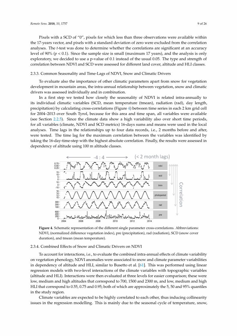
In a first step we tested how closely the seasonality of NDVI is related intra-annually toits individual climatic variables (SCD, mean temperature (tmean), radiation (rad), day length,precipitation) by calculating cross-correlations (Figure 4) between time series in each 2 km grid cellfor 2004–2013 over South Tyrol, because for this area and time span, all variables were available(see Section 2.2.5). Since the climate data show a high variability also over short time periods,for all variables (climate, NDVI and SCD metrics) 16-days sums and means were used in the localanalyses. Time lags in the relationships up to four data records, i.e., 2 months before and after,were tested. The time lag for the maximum correlation between the variables was identified bytaking the 16-day-time-step with the highest absolute correlation. Finally, the results were assessed independency of altitude using 100 m altitude classes.

Remote Sens. 2018, 10, x FOR PEER REVIEW    9 of 27 

2.3.3. Common Seasonality and Time‐Lags of NDVI, Snow and Climatic Drivers   

To evaluate also  the  importance of other climatic parameters apart  from snow for vegetation 

development in mountain areas, the intra‐annual relationship between vegetation, snow and climatic 

drivers was assessed individually and in combination.   

In a  first  step we  tested how  closely  the  seasonality of NDVI  is  related  intra‐annually  to  its 

individual  climatic  variables  (SCD,  mean  temperature  (tmean),  radiation  (rad),  day  length, 

precipitation) by calculating cross‐correlations (Figure 4) between time series in each 2 km grid cell 

for 2004–2013 over South Tyrol, because for this area and time span, all variables were available (see 

Section 2.2.5). Since  the  climate data  show a high variability also over  short  time periods,  for all 

variables (climate, NDVI and SCD metrics) 16‐days sums and means were used in the local analyses. 

Time lags in the relationships up to four data records, i.e., 2 months before and after, were tested. The 

time lag for the maximum correlation between the variables was identified by taking the 16‐day‐time‐

step with the highest absolute correlation. Finally, the results were assessed in dependency of altitude 

using 100 m altitude classes. 

 

Figure 4. Schematic representation of the different single parameter cross‐correlations. Abbreviations: 

NDVI, (normalized difference vegetation index), pre (precipitation), rad (radiation), SCD (snow cover 

duration), and tmean (mean temperature). 

2.3.4. Combined Effects of Snow and Climatic Drivers on NDVI   

To  account  for  interactions,  i.e.,  to  evaluate  the  combined  intra‐annual  effects  of  climate 

variability on vegetation phenology, NDVI anomalies were associated to snow and climate parameter 

variabilities  in dependency of altitude and HLI, similar  to Busetto et al. [61]. This was performed 

using linear regression models with two‐level interactions of the climate variables with topographic 

variables (altitude and HLI). Interactions were then evaluated at three levels for easier comparison; 

these were  low, medium  and high  altitudes  that  correspond  to  700,  1500  and  2300 m,  and  low, 

medium and high HLI that correspond to 0.55, 0.75 and 0.95; both of which are approximately the 5, 

50 and 95% quantiles in the study region.   

Climate variables are expected to be highly correlated to each other, thus inducing collinearity 

issues in the regression modelling. This is mainly due to the seasonal cycle of temperature, snow, and 

radiation.  To  remove  collinearity,  all  variables  (including  the  response  variable)  were  first 

deseasonalized for each grid cell using penalized cyclic splines (mgcv‐package in R): 

yij = f(doyj) + εij,  (1)

where yij is a variable (NDVI, SCD, …) at year i and 16‐day group j, f is a cyclic function, and doyj is 

the day‐of‐year. The residuals εij are the deseasonalized values, hereafter denoted with prefix d.   

Then for each 16‐day group separately, dNDVI was regressed on climate variables, altitude, HLI, 

and  two‐way  interactions between  climate and altitude as well as  climate and HLI. All available 

Figure 4. Schematic representation of the different single parameter cross-correlations. Abbreviations:NDVI, (normalized difference vegetation index), pre (precipitation), rad (radiation), SCD (snow coverduration), and tmean (mean temperature).

2.3.4. Combined Effects of Snow and Climatic Drivers on NDVI

To account for interactions, i.e., to evaluate the combined intra-annual effects of climate variabilityon vegetation phenology, NDVI anomalies were associated to snow and climate parameter variabilitiesin dependency of altitude and HLI, similar to Busetto et al. [61]. This was performed using linearregression models with two-level interactions of the climate variables with topographic variables(altitude and HLI). Interactions were then evaluated at three levels for easier comparison; these werelow, medium and high altitudes that correspond to 700, 1500 and 2300 m, and low, medium and highHLI that correspond to 0.55, 0.75 and 0.95; both of which are approximately the 5, 50 and 95% quantilesin the study region.

Climate variables are expected to be highly correlated to each other, thus inducing collinearityissues in the regression modelling. This is mainly due to the seasonal cycle of temperature, snow,

Remote Sens. 2018, 10, 1757 10 of 26

and radiation. To remove collinearity, all variables (including the response variable) were firstdeseasonalized for each grid cell using penalized cyclic splines (mgcv-package in R):

yij = f (doyj) + εij, (1)

where yij is a variable (NDVI, SCD, . . . ) at year i and 16-day group j, f is a cyclic function, and doyj isthe day-of-year. The residuals εij are the deseasonalized values, hereafter denoted with prefix d.

Then for each 16-day group separately, dNDVI was regressed on climate variables, altitude, HLI,and two-way interactions between climate and altitude as well as climate and HLI. All availableclimate variables were used, except for precipitation, because the cross-correlation analysis beforeshowed no influence. The regression model was run using 50% of the data as training and the other50% as test set (pixels were randomly selected for each 16-day group). The model formula is as follows:

dNDVIsi = β0 + β1dSCDsi + β2dTmeansi + β3dRadsi + β4WinterSCDsi + β5Altitudes + β6

HLIs + Altitudes(γ1dSCDsi + γ2dTmeansi + γ3dRadsi + γ4WinterSCDsi) + HLIs(δ1

dSCDsi + δ2dTmeansi + δ3dRadsi + δ4WinterSCDsi) + εsi,(2)

where d* denotes deseasonalized variables, s is a pixel index, i is year, β are the main effects, γ and δ areinteractions with altitude and HLI, WinterSCD is the SCD of the previous winter (December-February;variable only included in March-November models), and εsi ~N(0, σ2) errors [105]. Model selectionwas not performed, in order to keep models comparable across the 16-day groups. Instead we chose amultiplicity adjustment, and p-values for the coefficients were adjusted for multiple testing (23 models).The total number of estimated parameters for each model was 13 (or 16 if with WinterSCD) and thetotal number of observations in the training set varied between 7491 and 28,157 depending on 16-daygroup (less data available in winter because of cloud cover), so overfitting was not considered an issue.This was further confirmed by the small differences between training and test data in the evaluation ofmodel metrics.

3. Results

3.1. Temporal and Spatial Variabilities of Vegetation Phenology and Snow Metrics

3.1.1. Vegetation

SOS maps of alpine vegetation were derived for most years up to an elevation of 2700 m, while forthe remaining high alpine areas the available data was mostly too scarce to perform a statistical analysisdue to snow and cloud cover. Approaches adapted even further to the characteristics of these highaltitudes vegetation signals and noise might be necessary to describe these biomes. Also, the incompleteMODIS time series of the year 2000 proofed to be unreliable to derive phenological metrics.

The derived yearly SOS maps show a high variability with SOS values ranging from 30 to 212(median = DOY 109.5). Spatial variability is characterized by distinct small-scale patterns that aretracing altitude (see Figure 5). On average over all years, median SOS at different altitudes (100–2700 m)has a time lag of up to 57 days, with median SOS being delayed on average by 2.5 days per 100 m step(adjusted R2 = 0.90, p-value < 0.001). This tendency is not valid for the very low altitude ranges from200–800 m, where SOS is stable around DOY 106 or even a little delayed towards lower ranges (seeFigure S2). The year-to-year variability of median SOS in different altitudes follows a bell shape with16 to 25 days below 800 m and above 1600 m, and its maximum around 30 days from 1100 m to 1400 m.

To test whether slope and aspect related warming and cooling influences vegetation development,the SOS was averaged for the four different HLI and 29 elevation classes. In Figure S2, the SOS curves ofthe different HLI classes are displayed for each year and the entire altitudinal range, illustrating that thevariability between HLI classes in our data sets is small (standard deviation σ = 2.59 days) comparedto the intra-annual variability (σ = 7.19 days) as well as to the effects of altitude on SOS (σ = 18.3 days).

Remote Sens. 2018, 10, 1757 11 of 26

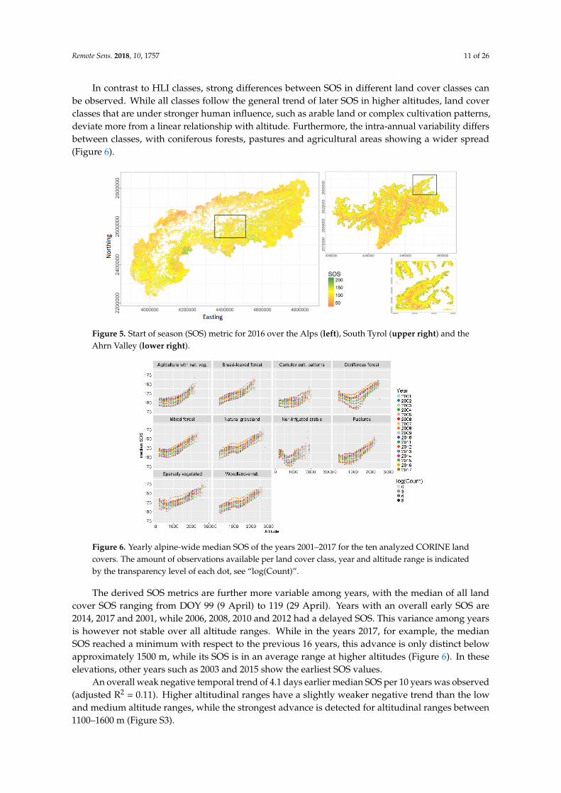
In contrast to HLI classes, strong differences between SOS in different land cover classes canbe observed. While all classes follow the general trend of later SOS in higher altitudes, land coverclasses that are under stronger human influence, such as arable land or complex cultivation patterns,deviate more from a linear relationship with altitude. Furthermore, the intra-annual variability differsbetween classes, with coniferous forests, pastures and agricultural areas showing a wider spread(Figure 6).Remote Sens. 2018, 10, x FOR PEER REVIEW    11 of 27 

 

Figure 5. Start of season (SOS) metric for 2016 over the Alps (left), South Tyrol (upper right) and the 

Ahrn Valley (lower right). 

 

Figure 6. Yearly alpine‐wide median SOS of the years 2001–2017 for the ten analyzed CORINE land 

covers. The amount of observations available per land cover class, year and altitude range is indicated 

by the transparency level of each dot, see “log(Count)”. 

The derived SOS metrics are further more variable among years, with the median of all  land 

cover SOS ranging from DOY 99 (9 April) to 119 (29 April). Years with an overall early SOS are 2014, 

2017 and 2001, while 2006, 2008, 2010 and 2012 had a delayed SOS. This variance among years  is 

however not stable over all altitude ranges. While in the years 2017, for example, the median SOS 

reached  a minimum with  respect  to  the  previous  16  years,  this  advance  is  only  distinct  below 

approximately 1500 m, while its SOS is in an average range at higher altitudes (Figure 6). In these 

elevations, other years such as 2003 and 2015 show the earliest SOS values. 

An  overall weak negative  temporal  trend  of  4.1 days  earlier median  SOS per  10  years was 

observed (adjusted R2 = 0.11). Higher altitudinal ranges have a slightly weaker negative trend than 

the low and medium altitude ranges, while the strongest advance is detected for altitudinal ranges 

between 1100–1600 m (Figure S3). 

Alpine‐wide monthly mean NDVI maps were available from February 2000 to June 2017. The 

median NDVI maps show a strong negative relationship (adjusted R2 = 0.77, p‐value < 0.001) with 

altitude, decreasing on average by 0.02 median NDVI per 100 m step. This relationship is however 

highly variable between different vegetation classes and not valid for the low altitudes below 1000 

m, where NDVI slightly increases with altitude (Figure S4).   

Figure 5. Start of season (SOS) metric for 2016 over the Alps (left), South Tyrol (upper right) and theAhrn Valley (lower right).

Remote Sens. 2018, 10, x FOR PEER REVIEW    11 of 27 

 

Figure 5. Start of season (SOS) metric for 2016 over the Alps (left), South Tyrol (upper right) and the 

Ahrn Valley (lower right). 

 

Figure 6. Yearly alpine‐wide median SOS of the years 2001–2017 for the ten analyzed CORINE land 

covers. The amount of observations available per land cover class, year and altitude range is indicated 

by the transparency level of each dot, see “log(Count)”. 

The derived SOS metrics are further more variable among years, with the median of all  land 

cover SOS ranging from DOY 99 (9 April) to 119 (29 April). Years with an overall early SOS are 2014, 

2017 and 2001, while 2006, 2008, 2010 and 2012 had a delayed SOS. This variance among years  is 

however not stable over all altitude ranges. While in the years 2017, for example, the median SOS 

reached  a minimum with  respect  to  the  previous  16  years,  this  advance  is  only  distinct  below 

approximately 1500 m, while its SOS is in an average range at higher altitudes (Figure 6). In these 

elevations, other years such as 2003 and 2015 show the earliest SOS values. 

An  overall weak negative  temporal  trend  of  4.1 days  earlier median  SOS per  10  years was 

observed (adjusted R2 = 0.11). Higher altitudinal ranges have a slightly weaker negative trend than 

the low and medium altitude ranges, while the strongest advance is detected for altitudinal ranges 

between 1100–1600 m (Figure S3). 

Alpine‐wide monthly mean NDVI maps were available from February 2000 to June 2017. The 

median NDVI maps show a strong negative relationship (adjusted R2 = 0.77, p‐value < 0.001) with 

altitude, decreasing on average by 0.02 median NDVI per 100 m step. This relationship is however 

highly variable between different vegetation classes and not valid for the low altitudes below 1000 

m, where NDVI slightly increases with altitude (Figure S4).   

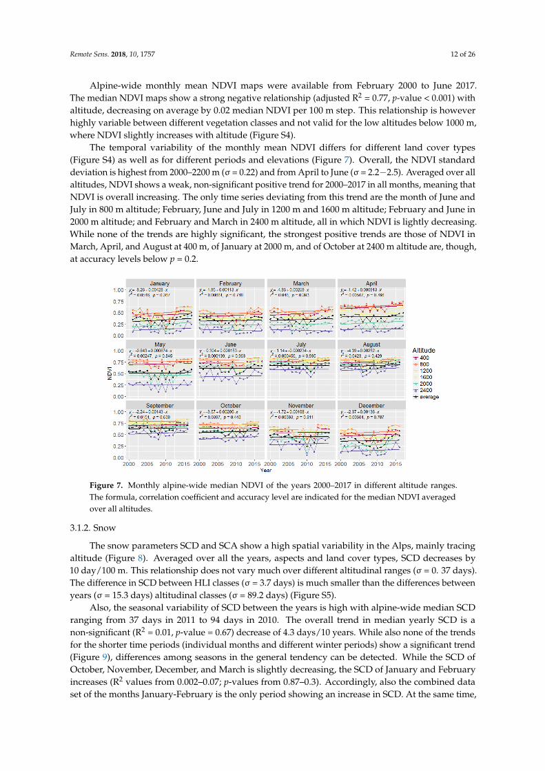
Figure 6. Yearly alpine-wide median SOS of the years 2001–2017 for the ten analyzed CORINE landcovers. The amount of observations available per land cover class, year and altitude range is indicatedby the transparency level of each dot, see “log(Count)”.

The derived SOS metrics are further more variable among years, with the median of all landcover SOS ranging from DOY 99 (9 April) to 119 (29 April). Years with an overall early SOS are2014, 2017 and 2001, while 2006, 2008, 2010 and 2012 had a delayed SOS. This variance among yearsis however not stable over all altitude ranges. While in the years 2017, for example, the medianSOS reached a minimum with respect to the previous 16 years, this advance is only distinct belowapproximately 1500 m, while its SOS is in an average range at higher altitudes (Figure 6). In theseelevations, other years such as 2003 and 2015 show the earliest SOS values.

An overall weak negative temporal trend of 4.1 days earlier median SOS per 10 years was observed(adjusted R2 = 0.11). Higher altitudinal ranges have a slightly weaker negative trend than the lowand medium altitude ranges, while the strongest advance is detected for altitudinal ranges between1100–1600 m (Figure S3).

Remote Sens. 2018, 10, 1757 12 of 26

Alpine-wide monthly mean NDVI maps were available from February 2000 to June 2017.The median NDVI maps show a strong negative relationship (adjusted R2 = 0.77, p-value < 0.001) withaltitude, decreasing on average by 0.02 median NDVI per 100 m step. This relationship is howeverhighly variable between different vegetation classes and not valid for the low altitudes below 1000 m,where NDVI slightly increases with altitude (Figure S4).

The temporal variability of the monthly mean NDVI differs for different land cover types(Figure S4) as well as for different periods and elevations (Figure 7). Overall, the NDVI standarddeviation is highest from 2000–2200 m (σ = 0.22) and from April to June (σ = 2.2−2.5). Averaged over allaltitudes, NDVI shows a weak, non-significant positive trend for 2000–2017 in all months, meaning thatNDVI is overall increasing. The only time series deviating from this trend are the month of June andJuly in 800 m altitude; February, June and July in 1200 m and 1600 m altitude; February and June in2000 m altitude; and February and March in 2400 m altitude, all in which NDVI is lightly decreasing.While none of the trends are highly significant, the strongest positive trends are those of NDVI inMarch, April, and August at 400 m, of January at 2000 m, and of October at 2400 m altitude are, though,at accuracy levels below p = 0.2.

Remote Sens. 2018, 10, x FOR PEER REVIEW    12 of 27 

The temporal variability of the monthly mean NDVI differs for different land cover types (Figure 

S4) as well as for different periods and elevations (Figure 7). Overall, the NDVI standard deviation is 

highest from 2000–2200 m (σ = 0.22) and from April to June (σ = 2.2−2.5). Averaged over all altitudes, 

NDVI shows a weak, non‐significant positive trend for 2000–2017 in all months, meaning that NDVI 

is overall increasing. The only time series deviating from this trend are the month of June and July in 

800 m altitude; February, June and July in 1200 m and 1600 m altitude; February and June in 2000 m 

altitude; and February and March in 2400 m altitude, all in which NDVI is lightly decreasing. While 

none of the trends are highly significant, the strongest positive trends are those of NDVI in March, 

April, and August at 400 m, of January at 2000 m, and of October at 2400 m altitude are, though, at 

accuracy levels below p = 0.2. 

 

Figure 7. Monthly alpine‐wide median NDVI of the years 2000–2017 in different altitude ranges. The 

formula, correlation coefficient and accuracy level are indicated for the median NDVI averaged over 

all altitudes. 

3.1.2. Snow 

The snow parameters SCD and SCA show a high spatial variability in the Alps, mainly tracing 

altitude (Figure 8). Averaged over all the years, aspects and land cover types, SCD decreases by 10 

day/100 m. This relationship does not vary much over different altitudinal ranges (σ = 0. 37 days). 

The difference  in  SCD  between HLI  classes  (σ  =  3.7 days)  is much  smaller  than  the differences 

between years (σ = 15.3 days) altitudinal classes (σ = 89.2 days) (Figure S5).   

Figure 8. Spatial patterns of yearly SCD for the years 2010 (left) and 2016 (right) over the Alps. 

Figure 7. Monthly alpine-wide median NDVI of the years 2000–2017 in different altitude ranges.The formula, correlation coefficient and accuracy level are indicated for the median NDVI averagedover all altitudes.

3.1.2. Snow

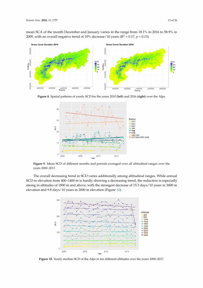
The snow parameters SCD and SCA show a high spatial variability in the Alps, mainly tracingaltitude (Figure 8). Averaged over all the years, aspects and land cover types, SCD decreases by10 day/100 m. This relationship does not vary much over different altitudinal ranges (σ = 0. 37 days).The difference in SCD between HLI classes (σ = 3.7 days) is much smaller than the differences betweenyears (σ = 15.3 days) altitudinal classes (σ = 89.2 days) (Figure S5).

Also, the seasonal variability of SCD between the years is high with alpine-wide median SCDranging from 37 days in 2011 to 94 days in 2010. The overall trend in median yearly SCD is anon-significant (R2 = 0.01, p-value = 0.67) decrease of 4.3 days/10 years. While also none of the trendsfor the shorter time periods (individual months and different winter periods) show a significant trend(Figure 9), differences among seasons in the general tendency can be detected. While the SCD ofOctober, November, December, and March is slightly decreasing, the SCD of January and Februaryincreases (R2 values from 0.002–0.07; p-values from 0.87–0.3). Accordingly, also the combined dataset of the months January-February is the only period showing an increase in SCD. At the same time,

Remote Sens. 2018, 10, 1757 13 of 26

mean SCA of the month December and January varies in the range from 18.1% in 2016 to 58.9% in2009, with an overall negative trend of 10% decrease/10 years (R2 = 0.17, p = 0.13).

Remote Sens. 2018, 10, x FOR PEER REVIEW    12 of 27 

The temporal variability of the monthly mean NDVI differs for different land cover types (Figure 

S4) as well as for different periods and elevations (Figure 7). Overall, the NDVI standard deviation is 

highest from 2000–2200 m (σ = 0.22) and from April to June (σ = 2.2−2.5). Averaged over all altitudes, 

NDVI shows a weak, non‐significant positive trend for 2000–2017 in all months, meaning that NDVI 

is overall increasing. The only time series deviating from this trend are the month of June and July in 

800 m altitude; February, June and July in 1200 m and 1600 m altitude; February and June in 2000 m 

altitude; and February and March in 2400 m altitude, all in which NDVI is lightly decreasing. While 

none of the trends are highly significant, the strongest positive trends are those of NDVI in March, 

April, and August at 400 m, of January at 2000 m, and of October at 2400 m altitude are, though, at 

accuracy levels below p = 0.2. 

 

Figure 7. Monthly alpine‐wide median NDVI of the years 2000–2017 in different altitude ranges. The 

formula, correlation coefficient and accuracy level are indicated for the median NDVI averaged over 

all altitudes. 

3.1.2. Snow 

The snow parameters SCD and SCA show a high spatial variability in the Alps, mainly tracing 

altitude (Figure 8). Averaged over all the years, aspects and land cover types, SCD decreases by 10 

day/100 m. This relationship does not vary much over different altitudinal ranges (σ = 0. 37 days). 

The difference  in  SCD  between HLI  classes  (σ  =  3.7 days)  is much  smaller  than  the differences 

between years (σ = 15.3 days) altitudinal classes (σ = 89.2 days) (Figure S5).   

Figure 8. Spatial patterns of yearly SCD for the years 2010 (left) and 2016 (right) over the Alps. Figure 8. Spatial patterns of yearly SCD for the years 2010 (left) and 2016 (right) over the Alps.

Remote Sens. 2018, 10, x FOR PEER REVIEW    13 of 27 

Also, the seasonal variability of SCD between the years is high with alpine‐wide median SCD 

ranging from 37 days in 2011 to 94 days in 2010. The overall trend in median yearly SCD is a non‐

significant (R2 = 0.01, p‐value = 0.67) decrease of 4.3 days/10 years. While also none of the trends for 

the shorter time periods (individual months and different winter periods) show a significant trend 

(Figure 9), differences among seasons  in  the general  tendency can be detected. While  the SCD of 

October, November, December, and March is slightly decreasing, the SCD of January and February 

increases (R2 values from 0.002–0.07; p‐values from 0.87–0.3). Accordingly, also the combined data set 

of the months January‐February is the only period showing an increase in SCD. At the same time, 

mean SCA of the month December and January varies in the range from 18.1% in 2016 to 58.9% in 

2009, with an overall negative trend of 10% decrease/10 years (R2 = 0.17, p = 0.13). 

 

Figure 9: Mean SCD of different months and periods averaged over all altitudinal ranges over the 

years 2000–2017. 

The overall decreasing trend in SCD varies additionally among altitudinal ranges. While annual 

SCD in elevation from 400–1400 m is hardly showing a decreasing trend, the reduction is especially 

strong in altitudes of 1800 m and above, with the strongest decrease of 15.3 days/10 years in 3000 m 

elevation and 9.8 days/10 years in 2000 m elevation (Figure 10). 

 

Figure 10: Yearly median SCD of the Alps in ten different altitudes over the years 2000–2017. 

3.2. Inter‐Annual Relationship between Monthly SCD and Mean NDVI 

The analysis of the inter‐annual relationship between the monthly SCD and the average NDVI 

of the respective month shows strong significant negative correlations (r < −0.5, p < 0.1) for 5–37% of 

all vegetated pixels of the different month‐month analyses for which enough pairwise observations 

were available, with a maximum in the winter month (December to April) (see for example Figure 

Figure 9. Mean SCD of different months and periods averaged over all altitudinal ranges over theyears 2000–2017.

The overall decreasing trend in SCD varies additionally among altitudinal ranges. While annualSCD in elevation from 400–1400 m is hardly showing a decreasing trend, the reduction is especiallystrong in altitudes of 1800 m and above, with the strongest decrease of 15.3 days/10 years in 3000 melevation and 9.8 days/10 years in 2000 m elevation (Figure 10).

Remote Sens. 2018, 10, x FOR PEER REVIEW    13 of 27 

Also, the seasonal variability of SCD between the years is high with alpine‐wide median SCD 

ranging from 37 days in 2011 to 94 days in 2010. The overall trend in median yearly SCD is a non‐

significant (R2 = 0.01, p‐value = 0.67) decrease of 4.3 days/10 years. While also none of the trends for 

the shorter time periods (individual months and different winter periods) show a significant trend 

(Figure 9), differences among seasons  in  the general  tendency can be detected. While  the SCD of 

October, November, December, and March is slightly decreasing, the SCD of January and February 

increases (R2 values from 0.002–0.07; p‐values from 0.87–0.3). Accordingly, also the combined data set 

of the months January‐February is the only period showing an increase in SCD. At the same time, 

mean SCA of the month December and January varies in the range from 18.1% in 2016 to 58.9% in 

2009, with an overall negative trend of 10% decrease/10 years (R2 = 0.17, p = 0.13). 

 

Figure 9: Mean SCD of different months and periods averaged over all altitudinal ranges over the 

years 2000–2017. 

The overall decreasing trend in SCD varies additionally among altitudinal ranges. While annual 

SCD in elevation from 400–1400 m is hardly showing a decreasing trend, the reduction is especially 

strong in altitudes of 1800 m and above, with the strongest decrease of 15.3 days/10 years in 3000 m 

elevation and 9.8 days/10 years in 2000 m elevation (Figure 10). 

 

Figure 10: Yearly median SCD of the Alps in ten different altitudes over the years 2000–2017. 

3.2. Inter‐Annual Relationship between Monthly SCD and Mean NDVI 

The analysis of the inter‐annual relationship between the monthly SCD and the average NDVI 

of the respective month shows strong significant negative correlations (r < −0.5, p < 0.1) for 5–37% of 

all vegetated pixels of the different month‐month analyses for which enough pairwise observations 

were available, with a maximum in the winter month (December to April) (see for example Figure 

Figure 10. Yearly median SCD of the Alps in ten different altitudes over the years 2000–2017.

Remote Sens. 2018, 10, 1757 14 of 26

3.2. Inter-Annual Relationship between Monthly SCD and Mean NDVI

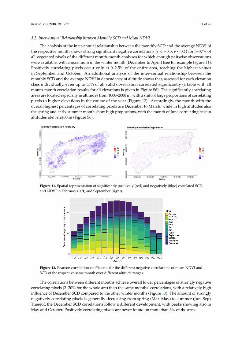
The analysis of the inter-annual relationship between the monthly SCD and the average NDVI ofthe respective month shows strong significant negative correlations (r < −0.5, p < 0.1) for 5–37% ofall vegetated pixels of the different month-month analyses for which enough pairwise observationswere available, with a maximum in the winter month (December to April) (see for example Figure 11).Positively correlating pixels occur only at 0–2.5% of the entire area, reaching the highest valuesin September and October. An additional analysis of the inter-annual relationship between themonthly SCD and the average NDVI in dependency of altitude shows that, assessed for each elevationclass individually, even up to 55% of all valid observation correlated significantly (a table with allmonth-month correlation results for all elevations is given in Figure S6). The significantly correlatingareas are located especially in altitudes from 1000–2000 m, with a shift of large proportions of correlatingpixels to higher elevations in the course of the year (Figure 12). Accordingly, the month with theoverall highest percentages of correlating pixels are December to March, while in high altitudes alsothe spring and early summer month show high proportions, with the month of June correlating best inaltitudes above 2400 m (Figure S6).

Remote Sens. 2018, 10, x FOR PEER REVIEW    14 of 27 

11). Positively correlating pixels occur only at 0–2.5% of the entire area, reaching the highest values 

in  September  and October. An  additional  analysis  of  the  inter‐annual  relationship  between  the 

monthly  SCD  and  the  average NDVI  in  dependency  of  altitude  shows  that,  assessed  for  each 

elevation class individually, even up to 55% of all valid observation correlated significantly (a table 

with all month‐month correlation results for all elevations is given in Figure S6). The significantly 

correlating areas are located especially in altitudes from 1000–2000 m, with a shift of large proportions 

of correlating pixels to higher elevations in the course of the year (Figure 12). Accordingly, the month 

with  the overall highest percentages of  correlating pixels  are December  to March, while  in high 

altitudes also the spring and early summer month show high proportions, with the month of June 

correlating best in altitudes above 2400 m (Figure S6). 

Figure 11. Spatial representation of significantly positively (red) and negatively (blue) correlated SCD 

and NDVI in February (left) and September (right). 

 

Figure 12. Pearson correlation coefficients for the different negative correlations of mean NDVI and 

SCD of the respective same month over different altitude ranges. 

The  correlations  between  different  months  achieve  overall  lower  percentages  of  strongly 

negative  correlating pixels  (2–20%  for  the whole are)  than  the  same months’  correlations, with a 

relatively high  influence of December SCD compared to the other winter months (Figure 13). The 

amount of strongly negatively correlating pixels is generally decreasing from spring (Mar–May) to 

summer  (Jun–Sep). Thereof,  the December SCD correlations  follow a different development, with 

peaks showing also in May and October. Positively correlating pixels are never found on more than 

3% of the area.   

Figure 11. Spatial representation of significantly positively (red) and negatively (blue) correlated SCDand NDVI in February (left) and September (right).

Remote Sens. 2018, 10, x FOR PEER REVIEW    14 of 27 

11). Positively correlating pixels occur only at 0–2.5% of the entire area, reaching the highest values 

in  September  and October. An  additional  analysis  of  the  inter‐annual  relationship  between  the 

monthly  SCD  and  the  average NDVI  in  dependency  of  altitude  shows  that,  assessed  for  each 

elevation class individually, even up to 55% of all valid observation correlated significantly (a table 

with all month‐month correlation results for all elevations is given in Figure S6). The significantly 

correlating areas are located especially in altitudes from 1000–2000 m, with a shift of large proportions 

of correlating pixels to higher elevations in the course of the year (Figure 12). Accordingly, the month 

with  the overall highest percentages of  correlating pixels  are December  to March, while  in high 

altitudes also the spring and early summer month show high proportions, with the month of June 

correlating best in altitudes above 2400 m (Figure S6). 

Figure 11. Spatial representation of significantly positively (red) and negatively (blue) correlated SCD 

and NDVI in February (left) and September (right). 

 

Figure 12. Pearson correlation coefficients for the different negative correlations of mean NDVI and 

SCD of the respective same month over different altitude ranges. 

The  correlations  between  different  months  achieve  overall  lower  percentages  of  strongly 

negative  correlating pixels  (2–20%  for  the whole are)  than  the  same months’  correlations, with a 

relatively high  influence of December SCD compared to the other winter months (Figure 13). The 

amount of strongly negatively correlating pixels is generally decreasing from spring (Mar–May) to 

summer  (Jun–Sep). Thereof,  the December SCD correlations  follow a different development, with 

peaks showing also in May and October. Positively correlating pixels are never found on more than 

3% of the area.   

Figure 12. Pearson correlation coefficients for the different negative correlations of mean NDVI andSCD of the respective same month over different altitude ranges.

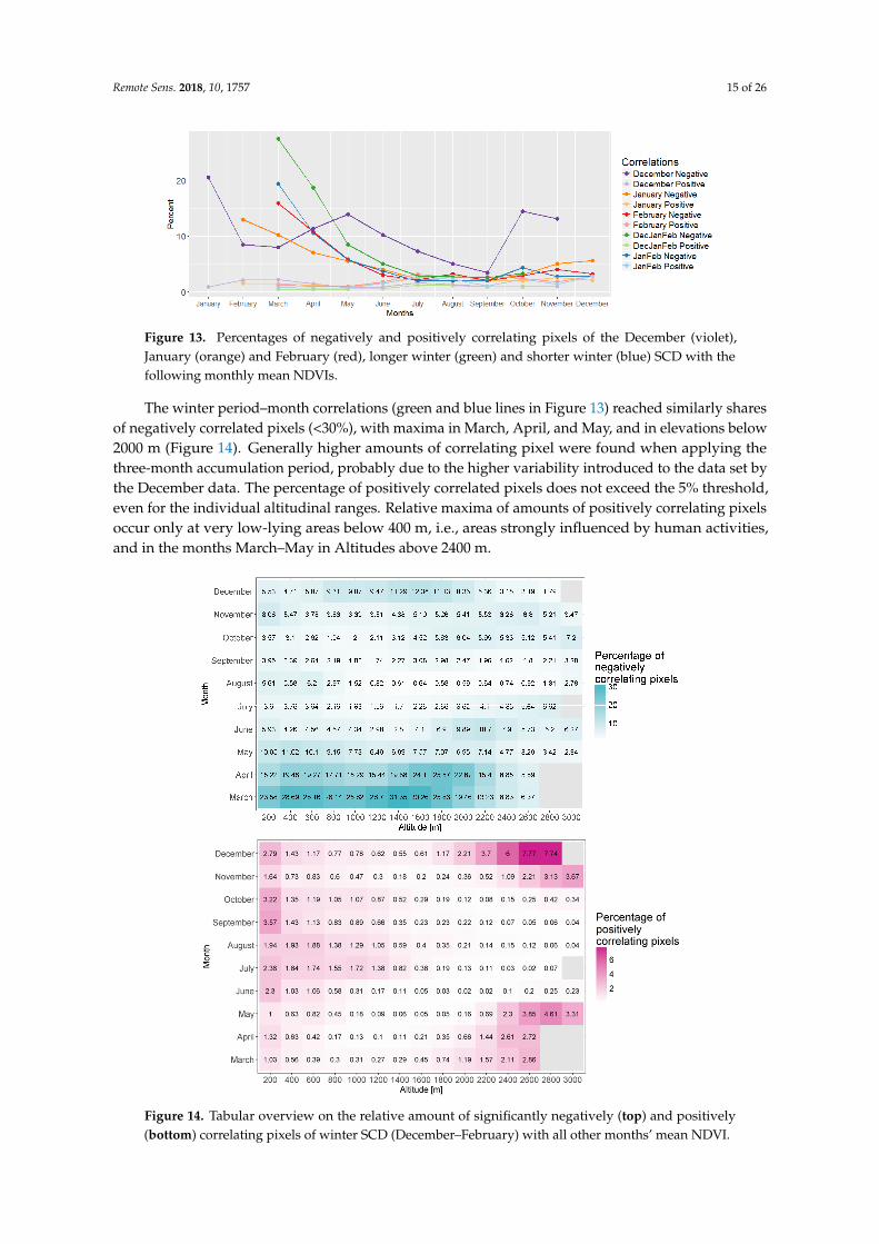
The correlations between different months achieve overall lower percentages of strongly negativecorrelating pixels (2–20% for the whole are) than the same months’ correlations, with a relatively highinfluence of December SCD compared to the other winter months (Figure 13). The amount of stronglynegatively correlating pixels is generally decreasing from spring (Mar–May) to summer (Jun–Sep).Thereof, the December SCD correlations follow a different development, with peaks showing also inMay and October. Positively correlating pixels are never found on more than 3% of the area.

Remote Sens. 2018, 10, 1757 15 of 26Remote Sens. 2018, 10, x FOR PEER REVIEW    15 of 27 

Figure  13.  Percentages  of  negatively  and  positively  correlating  pixels  of  the  December  (violet), 

January (orange) and February (red), longer winter (green) and shorter winter (blue) SCD with the 

following monthly mean NDVIs. 

The winter period–month  correlations  (green  and blue  lines  in Figure  13)  reached  similarly 

shares  of  negatively  correlated  pixels  (<30%), with maxima  in March,  April,  and May,  and  in 

elevations below 2000 m (Figure 14). Generally higher amounts of correlating pixel were found when 

applying the three‐month accumulation period, probably due to the higher variability introduced to 

the data set by the December data. The percentage of positively correlated pixels does not exceed the 

5% threshold, even for the individual altitudinal ranges. Relative maxima of amounts of positively 

correlating pixels occur only at very low‐lying areas below 400 m, i.e., areas strongly influenced by 

human activities, and in the months March–May in Altitudes above 2400 m. 

With regard  to  the period correlations differentiated among  land cover classes,  the  temporal 

development  is overall  the same with 21.1–40.1% of negatively correlating pixels  in March, 15.1–

28.7%  of  negatively  correlating  pixels  in April,  and  further decreasing  shares  of  the  alpine  area 

monthly mean NDVI being correlated to the winter SCD, with a minimum of on average only 2.7% 

of correlating pixels in September. However, differences between the land cover classes exist. Biomes 

consisting of rather herbaceous and gramineous species,  i.e., annual plants, such as  ‘pastures’  (on 

average 11.6% of NDVI‐SCD negatively correlated pixels in all month), ‘complex cultivation patterns’ 

(10.1%) or  ‘sparsely vegetated areas’  (9.6%)  show a higher  relationship with SCD  than  the  forest 

classes (7.1–7.9%) which have more slowly growing, woody vegetation. 

 

Figure 13. Percentages of negatively and positively correlating pixels of the December (violet),January (orange) and February (red), longer winter (green) and shorter winter (blue) SCD with thefollowing monthly mean NDVIs.

The winter period–month correlations (green and blue lines in Figure 13) reached similarly sharesof negatively correlated pixels (<30%), with maxima in March, April, and May, and in elevations below2000 m (Figure 14). Generally higher amounts of correlating pixel were found when applying thethree-month accumulation period, probably due to the higher variability introduced to the data set bythe December data. The percentage of positively correlated pixels does not exceed the 5% threshold,even for the individual altitudinal ranges. Relative maxima of amounts of positively correlating pixelsoccur only at very low-lying areas below 400 m, i.e., areas strongly influenced by human activities,and in the months March–May in Altitudes above 2400 m.

Remote Sens. 2018, 10, x FOR PEER REVIEW    15 of 27 

Figure  13.  Percentages  of  negatively  and  positively  correlating  pixels  of  the  December  (violet), 

January (orange) and February (red), longer winter (green) and shorter winter (blue) SCD with the 

following monthly mean NDVIs. 

The winter period–month  correlations  (green  and blue  lines  in Figure  13)  reached  similarly 

shares  of  negatively  correlated  pixels  (<30%), with maxima  in March,  April,  and May,  and  in 

elevations below 2000 m (Figure 14). Generally higher amounts of correlating pixel were found when 

applying the three‐month accumulation period, probably due to the higher variability introduced to 

the data set by the December data. The percentage of positively correlated pixels does not exceed the 

5% threshold, even for the individual altitudinal ranges. Relative maxima of amounts of positively 

correlating pixels occur only at very low‐lying areas below 400 m, i.e., areas strongly influenced by 

human activities, and in the months March–May in Altitudes above 2400 m. 

With regard  to  the period correlations differentiated among  land cover classes,  the  temporal 

development  is overall  the same with 21.1–40.1% of negatively correlating pixels  in March, 15.1–

28.7%  of  negatively  correlating  pixels  in April,  and  further decreasing  shares  of  the  alpine  area 

monthly mean NDVI being correlated to the winter SCD, with a minimum of on average only 2.7% 

of correlating pixels in September. However, differences between the land cover classes exist. Biomes 

consisting of rather herbaceous and gramineous species,  i.e., annual plants, such as  ‘pastures’  (on 

average 11.6% of NDVI‐SCD negatively correlated pixels in all month), ‘complex cultivation patterns’ 

(10.1%) or  ‘sparsely vegetated areas’  (9.6%)  show a higher  relationship with SCD  than  the  forest 

classes (7.1–7.9%) which have more slowly growing, woody vegetation. 

 

Remote Sens. 2018, 10, x FOR PEER REVIEW    16 of 27 

 

Figure 14. Tabular overview on the relative amount of significantly negatively (top) and positively 

(bottom) correlating pixels of winter SCD (December–February) with all other months’ mean NDVI. 

3.3. Intra‐Annual Relationships: Common Seasonality of Vegetation Activity and Climate 

The seasonality of NDVI in South Tyrol correlated best with the yearly seasonality of different 

climate variables depending on altitude (Figure 15). In the lowest altitudes up to 300 m, NDVI was 

correlated highest with radiation (purple) and temperature (orange), then until 700 m almost only to 

temperature. From 700 m to 2000 m the share of pixels where NDVI was correlated best to SCD (blue) 

increased continuously reaching 70%, while at the same time the share of pixels correlating best to 

temperature decreased to 25%. Across all altitudes from 300 m onwards, approximately 5% of pixels 

had the best correlation of NDVI to day length (green). While precipitation was also compared, its 

correlations with NDVI were always lower than the best of the other four variables, and so it is not 

present in the figure. 

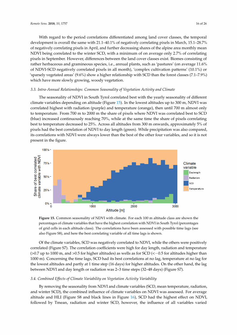
Figure 15. Common seasonality of NDVI with climate. For each 100 m altitude class are shown the 

percentages  of  climate  variables  that  have  the  highest  correlation  with  NDVI  in  South  Tyrol 

(percentages of grid cells in each altitude class). The correlations have been assessed with possible 

time lags (see also Figure S8), and here the best correlating variable of all time lags is shown. 

Of  the  climate  variables,  SCD  was  negatively  correlated  to  NDVI,  while  the  others  were 

positively correlated (Figure S7). The correlation coefficients were high for day length, radiation and 

temperature (>0.7 up to 1000 m, and >0.5 for higher altitudes) as wells as for SCD (<−0.5 for altitudes 

higher than 1000 m). Concerning the time lags, SCD had its best correlations at no lag, temperature 

Figure 14. Tabular overview on the relative amount of significantly negatively (top) and positively(bottom) correlating pixels of winter SCD (December–February) with all other months’ mean NDVI.

Remote Sens. 2018, 10, 1757 16 of 26

With regard to the period correlations differentiated among land cover classes, the temporaldevelopment is overall the same with 21.1–40.1% of negatively correlating pixels in March, 15.1–28.7%of negatively correlating pixels in April, and further decreasing shares of the alpine area monthly meanNDVI being correlated to the winter SCD, with a minimum of on average only 2.7% of correlatingpixels in September. However, differences between the land cover classes exist. Biomes consisting ofrather herbaceous and gramineous species, i.e., annual plants, such as ‘pastures’ (on average 11.6%of NDVI-SCD negatively correlated pixels in all month), ‘complex cultivation patterns’ (10.1%) or‘sparsely vegetated areas’ (9.6%) show a higher relationship with SCD than the forest classes (7.1–7.9%)which have more slowly growing, woody vegetation.

3.3. Intra-Annual Relationships: Common Seasonality of Vegetation Activity and Climate

The seasonality of NDVI in South Tyrol correlated best with the yearly seasonality of differentclimate variables depending on altitude (Figure 15). In the lowest altitudes up to 300 m, NDVI wascorrelated highest with radiation (purple) and temperature (orange), then until 700 m almost onlyto temperature. From 700 m to 2000 m the share of pixels where NDVI was correlated best to SCD(blue) increased continuously reaching 70%, while at the same time the share of pixels correlatingbest to temperature decreased to 25%. Across all altitudes from 300 m onwards, approximately 5% ofpixels had the best correlation of NDVI to day length (green). While precipitation was also compared,its correlations with NDVI were always lower than the best of the other four variables, and so it is notpresent in the figure.

Remote Sens. 2018, 10, x FOR PEER REVIEW    16 of 27 

 

Figure 14. Tabular overview on the relative amount of significantly negatively (top) and positively 

(bottom) correlating pixels of winter SCD (December–February) with all other months’ mean NDVI. 

3.3. Intra‐Annual Relationships: Common Seasonality of Vegetation Activity and Climate 

The seasonality of NDVI in South Tyrol correlated best with the yearly seasonality of different 

climate variables depending on altitude (Figure 15). In the lowest altitudes up to 300 m, NDVI was 

correlated highest with radiation (purple) and temperature (orange), then until 700 m almost only to 

temperature. From 700 m to 2000 m the share of pixels where NDVI was correlated best to SCD (blue) 

increased continuously reaching 70%, while at the same time the share of pixels correlating best to 

temperature decreased to 25%. Across all altitudes from 300 m onwards, approximately 5% of pixels 

had the best correlation of NDVI to day length (green). While precipitation was also compared, its 

correlations with NDVI were always lower than the best of the other four variables, and so it is not 

present in the figure. 

Figure 15. Common seasonality of NDVI with climate. For each 100 m altitude class are shown the 

percentages  of  climate  variables  that  have  the  highest  correlation  with  NDVI  in  South  Tyrol 

(percentages of grid cells in each altitude class). The correlations have been assessed with possible 

time lags (see also Figure S8), and here the best correlating variable of all time lags is shown. 

Of  the  climate  variables,  SCD  was  negatively  correlated  to  NDVI,  while  the  others  were 

positively correlated (Figure S7). The correlation coefficients were high for day length, radiation and 

temperature (>0.7 up to 1000 m, and >0.5 for higher altitudes) as wells as for SCD (<−0.5 for altitudes 

higher than 1000 m). Concerning the time lags, SCD had its best correlations at no lag, temperature 

Figure 15. Common seasonality of NDVI with climate. For each 100 m altitude class are shown thepercentages of climate variables that have the highest correlation with NDVI in South Tyrol (percentagesof grid cells in each altitude class). The correlations have been assessed with possible time lags (seealso Figure S8), and here the best correlating variable of all time lags is shown.

Of the climate variables, SCD was negatively correlated to NDVI, while the others were positivelycorrelated (Figure S7). The correlation coefficients were high for day length, radiation and temperature(>0.7 up to 1000 m, and >0.5 for higher altitudes) as wells as for SCD (<−0.5 for altitudes higher than1000 m). Concerning the time lags, SCD had its best correlations at no lag, temperature at no lag forthe lowest altitudes and partly at 1 time step (16 days) for higher altitudes. On the other hand, the lagbetween NDVI and day length or radiation was 2–3 time steps (32–48 days) (Figure S7).

3.4. Combined Effects of Climate Variability on Vegetation Activity Variability

By removing the seasonality from NDVI and climate variables (SCD, mean temperature, radiation,and winter SCD), the combined influence of climate variables on NDVI was assessed. For averagealtitude and HLI (Figure S8 and black lines in Figure 16), SCD had the highest effect on NDVI,followed by Tmean, radiation and winter SCD, however, the influence of all variables varied

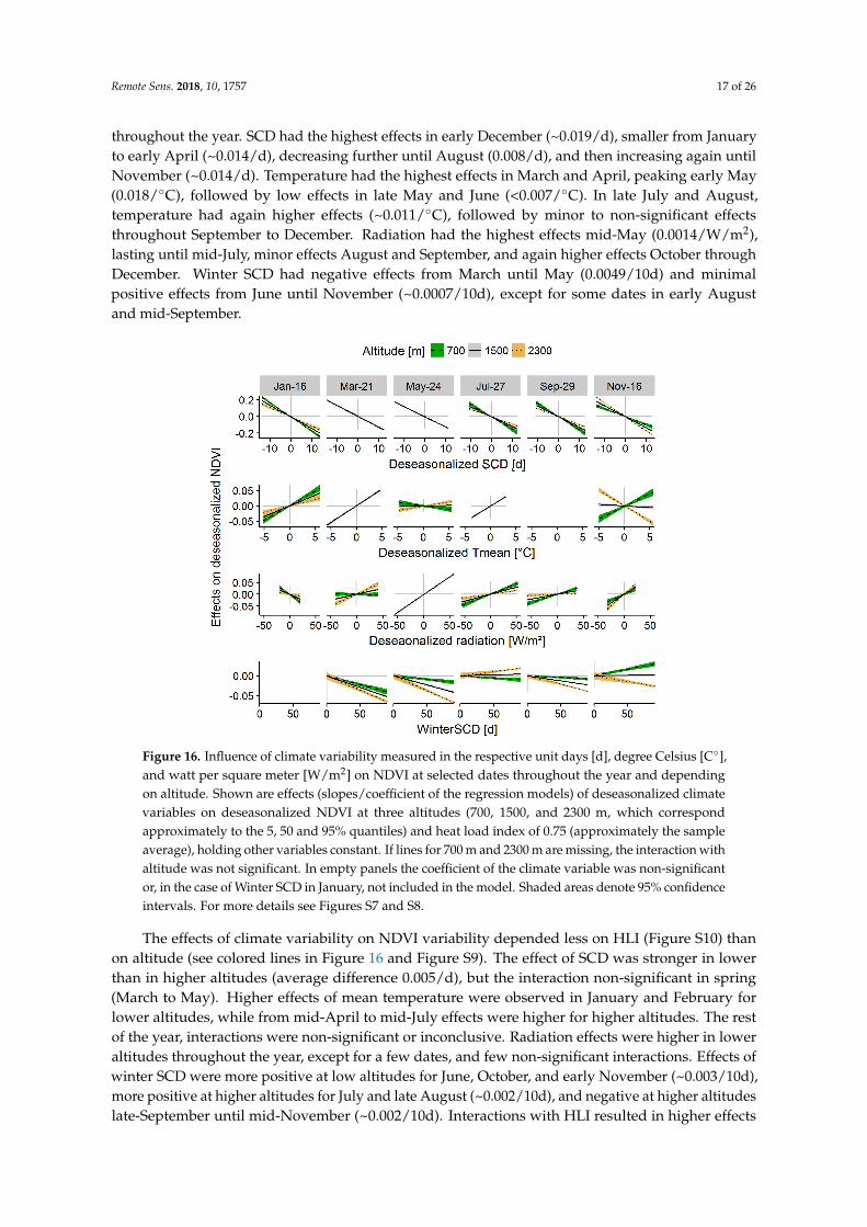
Remote Sens. 2018, 10, 1757 17 of 26

throughout the year. SCD had the highest effects in early December (~0.019/d), smaller from Januaryto early April (~0.014/d), decreasing further until August (0.008/d), and then increasing again untilNovember (~0.014/d). Temperature had the highest effects in March and April, peaking early May(0.018/◦C), followed by low effects in late May and June (<0.007/◦C). In late July and August,temperature had again higher effects (~0.011/◦C), followed by minor to non-significant effectsthroughout September to December. Radiation had the highest effects mid-May (0.0014/W/m2),lasting until mid-July, minor effects August and September, and again higher effects October throughDecember. Winter SCD had negative effects from March until May (0.0049/10d) and minimalpositive effects from June until November (~0.0007/10d), except for some dates in early Augustand mid-September.

Remote Sens. 2018, 10, x FOR PEER REVIEW    17 of 27 

at no lag for the lowest altitudes and partly at 1 time step (16 days) for higher altitudes. On the other 

hand, the lag between NDVI and day length or radiation was 2–3 time steps (32–48 days) (Figure S7). 

3.4. Combined Effects of Climate Variability on Vegetation Activity Variability 

By  removing  the  seasonality  from  NDVI  and  climate  variables  (SCD,  mean  temperature, 

radiation, and winter SCD), the combined influence of climate variables on NDVI was assessed. For 

average altitude and HLI  (Figure S8 and black  lines  in Figure 16), SCD had  the highest effect on 

NDVI, followed by Tmean, radiation and winter SCD, however, the influence of all variables varied 

throughout the year. SCD had the highest effects in early December (~0.019/d), smaller from January 

to early April (~0.014/d), decreasing further until August (0.008/d), and then increasing again until 

November (~0.014/d). Temperature had the highest effects in March and April, peaking early May 

(0.018/°C),  followed  by  low  effects  in  late May  and  June  (<0.007/°C).  In  late  July  and  August, 

temperature  had  again  higher  effects  (~0.011/°C),  followed  by  minor  to  non‐significant  effects 

throughout  September  to December.  Radiation  had  the  highest  effects mid‐May  (0.0014/W/m²), 

lasting until mid‐July, minor effects August and September, and again higher effects October through 

December. Winter SCD had negative effects from March until May (0.0049/10d) and minimal positive 

effects  from  June until November  (~0.0007/10d), except  for some dates  in early August and mid‐

September. 

 

Figure 16. Influence of climate variability measured  in the respective unit days [d], degree Celsius 

[C°], and watt per square meter [W/m2] on NDVI at selected dates throughout the year and depending 

on altitude. Shown are effects (slopes/coefficient of the regression models) of deseasonalized climate 

variables  on  deseasonalized NDVI  at  three  altitudes  (700,  1500,  and  2300 m, which  correspond 

approximately to the 5, 50 and 95% quantiles) and heat load index of 0.75 (approximately the sample 

average), holding other variables constant. If lines for 700 m and 2300 m are missing, the interaction 

with altitude was not significant.  In empty panels  the coefficient of  the climate variable was non‐

significant or, in the case of Winter SCD in January, not included in the model. Shaded areas denote 

95% confidence intervals. For more details see Figures S7 and S8. 

The effects of climate variability on NDVI variability depended less on HLI (Figure S10) than on 

altitude  (see colored  lines  in Figures 16 and S9). The effect of SCD was stronger  in  lower  than  in 

Figure 16. Influence of climate variability measured in the respective unit days [d], degree Celsius [C◦],and watt per square meter [W/m2] on NDVI at selected dates throughout the year and dependingon altitude. Shown are effects (slopes/coefficient of the regression models) of deseasonalized climatevariables on deseasonalized NDVI at three altitudes (700, 1500, and 2300 m, which correspondapproximately to the 5, 50 and 95% quantiles) and heat load index of 0.75 (approximately the sampleaverage), holding other variables constant. If lines for 700 m and 2300 m are missing, the interaction withaltitude was not significant. In empty panels the coefficient of the climate variable was non-significantor, in the case of Winter SCD in January, not included in the model. Shaded areas denote 95% confidenceintervals. For more details see Figures S7 and S8.

The effects of climate variability on NDVI variability depended less on HLI (Figure S10) thanon altitude (see colored lines in Figure 16 and Figure S9). The effect of SCD was stronger in lowerthan in higher altitudes (average difference 0.005/d), but the interaction non-significant in spring(March to May). Higher effects of mean temperature were observed in January and February forlower altitudes, while from mid-April to mid-July effects were higher for higher altitudes. The restof the year, interactions were non-significant or inconclusive. Radiation effects were higher in loweraltitudes throughout the year, except for a few dates, and few non-significant interactions. Effects ofwinter SCD were more positive at low altitudes for June, October, and early November (~0.003/10d),more positive at higher altitudes for July and late August (~0.002/10d), and negative at higher altitudeslate-September until mid-November (~0.002/10d). Interactions with HLI resulted in higher effects

Remote Sens. 2018, 10, 1757 18 of 26

of mean temperature for higher HLI for mid-February until late-April (average difference 0.005/◦C),and more negative effects of winter SCD for low HLI in March. For the other climate variables andother dates, interactions with HLI were mostly non-significant (Figure S10).

Since only half of the data was used to fit the models, the other half of the data could be used forvalidation purposes (Figure S11). Climate variability interacted with altitude and HLI could explainon average 30% of NDVI variation from late-October until late-May, and 9% on average for June untilearly-October. Explained variation was the highest in December and March with values around 40%.The differences between the training and the validation R2 were less 1.6%. Median absolute error(MAE) was around 0.08 from mid-November until mid-July, and around 0.06 otherwise. Differences inMAE between the training and validation set were less than 0.0017.

4. Discussion

4.1. Assessment of Spatiotemporal Patterns of Snow and Vegetation Phenology Variability

As expected, a strong dependency of vegetation and snow metrics on altitude is visible from thedata, with a delay of SOS of 2.5 days and a shortening of SCD of 10 days per 100 m. The only areasdeviating from this trend are situated in low elevations below 800 m, which are densely populatedvalley bottoms and therefore probably stronger influenced by human activities, as which might beoften be influenced by atmospheric inversion, i.e., deviating from the overall temperature patterns.While it has to be considered that the vegetation types occur at varying frequencies in differentelevation classes, it could be shown that vegetation in low lying areas and those under strongerhuman influence and more often consisting of annual plants (e.g., arable land, pastures and complexcultivation patterns) behaves distinctively different than more natural vegetation. The high variabilityof coniferous forest is an outlier in this respect and needs more investigation, e.g., by testing if thisvariance might be attributed to difficulties of snow cover mapping in forested areas. This effect isreduced in rather natural classes such as broadleaved forest, natural grasslands, and sparsely vegetatedareas. Additionally, elevation-dependent and intra-annual differences between land cover classes canbe observed.

Temporal developments of the analyzed metrics tend towards an earlier onset of vegetationgrowth of about 4 days/10 years, increasing monthly mean NDVI values in spring and late summer,as well as to shorter SCD of 4.3 days/10 years and a reduction in SCA. However, none of thesemetrics showed a statistically significant trend. This is most probably caused by the high intra-annualvariability presented in this study as well as by the insufficient length of the MODIS observations timeseries to derive robust trends [106]. Hence, the usage of a longer time series might be necessary toderive robust statistical measures, a requirement that hardly can be met at the moment due to theconcurrent need of a high spatial resolution.

Although none of the 17-year trends derived from the MODIS data is significant at the95% accuracy level, they are in the range of changes observed by the IPCC [107] and otherstudies [8,14,108,109]. Differences in these tendencies occur in different elevations and periods.While the SCD of January and February increased, SCD of October, November, December and Marchdecreased, pointing to a reduction of the snow cover period in the transition months between seasonsas well as a concentration of snow fall to a shorter time period. The simultaneous decrease of SCA inthe Alps in this period seems contradictory, but might indicate that also the ‘core winter’ is affected bywarming. These findings ask however for more investigations on the distribution and amount of snowin the alpine area, an aspect which is out of scope of this study.

The strongest advance is detected for altitudinal ranges between 1100–1600 m, which could bean indication for the enhancement of warming rates with elevation, so-called elevation-dependentwarming [50]. The fact that this tendency could not be observed for the highest altitude ranges could beaccounted to snow and cloud induced missing data in these ranges (see below). The high intra-annualvariability of vegetation metrics in elevation ranges from 1100 m–1500 m compared to other elevation

Remote Sens. 2018, 10, 1757 19 of 26

ranges as well as the described change in “early SOS years” around that altitude further indicatesan increased sensitivity of vegetation in this altitudinal range to different climatic changes and tointra-annual climate variability.

Analyzing the monthly mean NDVI time series in addition to SOS further revealed developmentsin vegetation activity throughout the vegetation period and in different altitudes. The high varianceof mean NDVI in the months April to June is in accordance to the detected SOS dates, and enablesa robust correlation analysis with its climatic drivers (see Sections 3.2–3.4). While the high varianceof NDVI in elevations from 2000–2200 m seems contradictory to the variance of the SOS, it can beprobably attributed to the quick and strong changes that alpine vegetation undergoes in these altitudes.The increase of NDVI metrics in low altitudes in March and April as well as in January and October inaltitudes above 2000 m indicate spatiotemporal variable shifts of vegetation periods in mountain areas.In this regard the combined use of SOS and NDVI metrics increased the information content extractedfrom the MODIS time series.

No SOS estimates could be derived for the very high altitudinal ranges due to the high amountof observations affected by clouds and snow, which is a limitation for the monitoring of ecosystemswhich are potentially very susceptive to climate change. Adapted LSP methods that allow for robustSOS estimation also given more frequent data gaps would be needed for analyzing these areas.Overcoming this constraint would also be beneficial for LSP assessments in boreal and polar regions(see e.g., [94,96,110]). Also, the expected influence of exposition on snow and vegetation phenology isnot traceable in the data set. The fact that the investigated metrics did not vary depending on HLImight indicate that the used spatial resolution of 250 m is still too coarse to capture habitat differencesthat are created by small-scale topographic variations, a shortcoming that was also detected in a studyusing similar data [111]. As discussed by Comola et al. [112], the effect of aspects become uncorrelatedand orientation differences average out at larger scales.

4.2. Derivation of Statistical Relationships between Vegetation Phenology and Snow Cover

In this study, different statistical techniques were used to assess different aspects of alpinevegetation variability such as seasonality and anomalies as well as possible causal relationships. As alogical relationship, for most valid mean NDVI and SCD matches, a generally negative correlationwas observed at the landscape scale, i.e., longer snow cover corresponds to lower NDVI. Furthermore,for years with a shorter SCD such as 2016 and 2017, earlier SOS values were observed, especially inlower altitudes, which is comparable with the results of similar, not earth observation-based studies(e.g., [113]).

In general, months and altitudinal ranges with higher inter-annual variability in snow cover showthe highest negative relationship of NDVI to SCD. The correlation strength is decreasing from winter(Dec–Mar) to spring (Mar–May) to summer (Jun–Sep). Weak positive correlations between winterSCDs and spring and late summer mean NDVIs in higher altitudes could point to a lagged waterstorage effect.

The overall highest number of correlating pixels in the same months’ NDVI and SCD mapsstress the direct influence snow cover can have on LSP, i.e., the high sensitivity of green-up to snowaccumulation and snow melt. However, two confounding effects could interact. While snow has aninhibiting effect on vegetation growth [68,94], snow also exacerbates the seasonal dampening of thevegetation signal, making it difficult to separate the green-up due to the emergence of leaves from anNDVI increase due to the snow disappearance.

The strength of the SCD-NDVI relationship differs further with altitude. Correlating areasare located especially in altitudes from 1000–2000 m, with a general tendency of upward movingcorrelating pixels throughout the vegetation period. Similarly, differences could be detected amongland cover classes. The direct influence of winter SCD on March NDVI was visible on about 30–40%percent of pasture and agricultural areas, but only on 20–25% of forest areas. This illustrates the abilityof the data sets to trace the highly variable vegetation responses to snow as a climatic driver in the

Remote Sens. 2018, 10, 1757 20 of 26

most sensitive altitudinal ranges. It was also shown, that using SCD data aggregated to two or threemonth achieved better results than using single month SCD, which is most probably related to theincreased necessary variance in the data set that is achieved by a longer integration period.

Given the low number of years investigated, as well as statistical limitations given wheninvestigating an explanatory variable that very often is close to zero, this share of explained varianceon the landscape scale is high and in line with similar studies [73,102,103]. However, further remotesensing based phenological metrics such as end of season, length of season and the first and last snowday could be applied to asses in more detail also the phenological mechanisms in the senescence phase,a process that is overall less good understood and modeled [18,114,115].

4.3. Assessment of the Common Seasonality and Combined Influence of Climate Parameters and Snow on Phenology

To understand the relative importance of snow cover variations as phenological driver withrespect to the other variables, a more detailed statistical analysis of vegetation metrics, snow coverand a range of climatic variables was performed on the limited area of South Tyrol. Therefore it wasshown, that mean temperature alone explains vegetation seasonality across all altitudes, but better inlower areas. SCD alone, on the other hand outperforms in higher altitudes. The transition altitudebetween these two dominating effects is also the elevation which showed the highest year-to-yearvariability in vegetation metrics (see Section 4.1). It can therefore be concluded, that in mountainousareas, snow and temperature can be combined to produce equally good results in phenology modelingacross all altitudes.

In the combined effects, SCD had the highest effect on NDVI. Overall, climate variability interactedwith altitude and HLI could explain on average 30% of NDVI variation from late-October until late-May,and 9% on average for June until early-October. Explained variation was the highest in December andMarch with values around 40%. The combined effects of winter SCD were negative from March untilMay, more positive at low altitudes for June, October, and early November, more positive at higheraltitudes for July and late August, and negative at higher altitudes late-September until mid-November.This shift of the peak of the effect might be an indication of a water storage effect; however, the effectwas several magnitudes lower compared to the other variables. As for the variability of snow andvegetation metrics, the effects of climate variability on NDVI variability depended less on HLI thanon altitude. As discussed above, this is likely a scale-dependent result, which is even reinforcedwith the resampling of all data to the 2 km spatial resolution [112]. Nevertheless, it seems that smallvariations in highly dynamic periods, such as the higher effects of mean temperature for higher HLI formid-February until late-April and more negative effects of winter SCD for low HLI in March, might bereinforced by exposition.

Overall the high variance explained by SCD stresses the importance of snow as a phenologicaldriver that might alter plant development even more strongly in the future. These findings enablealso a better interpretation of the outcomes of the analysis on the whole European Alps executedconsidering snow cover variations as the only driver of phenology (Section 3.2), imparting them a highvalidity even though only snow as climatic driver was analyzed.

5. Conclusions

In this study, we jointly analyzed the temporal and spatial variability of snow and plant phenologyon an alpine-wide scale at 250 m resolution. The presented regional analysis allows to assess thespatiotemporal patterns of earth-observation based snow and vegetation metrics over different landcovers, altitudes and topographic features, as well as to understand the relative importance of snowcover variations as phenology driver with respect to the other variables and in different elevations.Both snow and vegetation parameters showed clear patterns related to topography, with a delay ofSOS of about 2.5 days and an increment of 10 days in SCD per 100 m. No significant temporal trendsof earlier SOS as well as of shorter SCD could be detected on the alpine-wide scale, probably due to thehigh regional variability and insufficient length of the MODIS data set. The statistical interrelationships

Remote Sens. 2018, 10, 1757 21 of 26

of plant photosynthetic activity and its drivers revealed the high explanatory power of SCD, also incombination with other climatic drivers and especially in altitudes above 1000 m. However, the strengthof the correlations and the combined climate influence varies throughout the year and for differentaltitudes. While the time series used as a data base in this study is not long enough to derive statisticalrobust climate-relevant trends, it nevertheless stresses the relevance of monitoring mountain areas,which are among the regions of the globe that are warming the most, but for which at the same time,monitoring the rate and patterns of warming is challenging [49].

Supplementary Materials: The following are available online at http://www.mdpi.com/2072-4292/10/11/1757/s1,Figure S1: Illustration of the used NDVI time series winter gap filling approach for a pasture area. Figure S2:Yearly mean SOS of the years 2000–2017 for four HLI value ranges representing the quartiles of the data set,Figure S3: Median SOS over the Alps for the years 2001–2017 for different altitudes and the respective trendlines. The formula, correlation coefficient and accuracy level are indicated for the median SOS averaged over allaltitudes, Figure S4: Yearly alpine-wide median NDVI of the years 2000–2017 for the ten analyzed CORINE landcover, Figure S5: Yearly SCD of the years 2000–2017 for four HLI value ranges representing the quartiles of thedata set, Figure S6: Percentage of all negatively (top) and positively (bottom) correlated pixels between SCD andmean NDVI of the respective same month over the hydrological year (1 October–30 September), Figure S7: Resultsfrom cross-correlating 16-day values of NDVI with climate variables for all 2 km by 2 km grid cells in South Tyrolduring 2003–2012, Figure S8: Influence of climate variability on NDVI (normalized difference vegetation index),Figure S9: Influence of climate variability on NDVI (normalized difference vegetation index) at different altitudeclasses, Figure S10: Influence of climate variability on NDVI (normalized difference vegetation index) at differentHLI classes, Figure S11: Model metrics of regressing deseasonalized NDVI on deseasonalized climate variablesinteracted with altitude and HLI (heat load index).

Author Contributions: Conceptualization, S.A., M.C., A.M., M.Z. and C.N.; Data curation, S.A., M.M., L.D.G.and A.J.; Formal analysis, S.A., M.M. and G.F.; Funding acquisition, M.Z.; Writing—original draft, S.A.; Writing,review and editing, S.A., M.C., M.M., M.Z. and C.N.

Funding: This study was financially supported by the Autonomous Province of Bolzano/Bozen within theframe of the project MONALISA. Michael Matiu was receiving funding from the European Research Council(FP7/2007-2013, ERC GA282250) and was supported by the International Graduate School of Science andEngineering (IGSSE), funded by the German Excellence Initiative.

Acknowledgments: We are grateful to the MODIS team and the CORINE land cover team for making the datafreely available. The authors would like to thank the anonymous reviewers for their very constructive remarks.

Conflicts of Interest: The authors declare no conflict of interest. The funders had no role in the design of thestudy; in the collection, analyses, or interpretation of data; in the writing of the manuscript, or in the decision topublish the results.

References

1. Jarvis, P.G. The interpretation of the variations in leaf water potential and stomatal conductance found incanopies in the field. Philos. Trans. R. Soc. Lond. B 1976, 273, 593–610. [CrossRef]

2. Larcher, W. Physiological Plant Ecology: Ecophysiology and Stress Physiology of Functional Groups, 4th ed.;Springer: Heidelberg, Germany, 2003; ISBN 978-3-540-43516-7.

3. Scheifinger, H.; Menzel, A.; Koch, E.; Peter, C.; Ahas, R. Atmospheric mechanisms governing the spatial andtemporal variability of phenological phases in central Europe. Int. J. Climatol. 2002, 22, 1739–1755. [CrossRef]

4. Menzel, A. Trends in phenological phases in Europe between 1951 and 1996. Int. J. Biometeorol. 2000, 44,76–81. [CrossRef] [PubMed]

5. Menzel, A.; Fabian, P. Growing season extended in Europe. Nature 1999, 397, 659. [CrossRef]6. Van Vliet, A.J.H.; de Groot, R.S.; Bellens, Y.; Braun, P.; Bruegger, R.; Bruns, E.; Clevers, J.; Estreguil, C.;

Flechsig, M.; Jeanneret, F.; et al. The European Phenology Network. Int. J. Biometeorol. 2003, 47, 202–212.[CrossRef] [PubMed]

7. Betancourt, J.L.; Schwartz, M.D.; Breshears, D.D.; Cayan, D.R.; Dettinger, M.D.; Inouye, D.W.; Post, E.;Reed, B.C. Implementing a U.S. National Phenology Network. Eos Trans. AGU 2005, 86, 539. [CrossRef]

8. Menzel, A. European phenological response to climate change matches the warming pattern. Glob. Chang. Biol.2006, 12, 1969–1976. [CrossRef]

9. Schwartz, M.D.; Reed, B.C.; White, M.A. Assessing satellite derived start-of-season measures in theconterminous USA. Int. J. Climatol. 2002, 22, 1793–1805. [CrossRef]

Remote Sens. 2018, 10, 1757 22 of 26

10. Fisher, J.I.; Mustard, J.F.; Vadeboncoeur, M.A. Green leaf phenology at Landsat resolution: Scaling from thefield to the satellite. Remote Sens. Environ. 2006, 100, 265–279. [CrossRef]

11. Dunn, A.; de Beurs, K. Land surface phenology of North American mountain environments using moderateresolution imaging spectroradiometer data. Remote Sens. Environ. 2011, 115, 1220–1233. [CrossRef]

12. Gonsamo, A.; Chen, J.M.; Price, D.T.; Kurz, W.A.; Wu, C. Land surface phenology from optical satellitemeasurement and CO2 eddy covariance technique. J. Geophys. Res. 2012, 117, G03032. [CrossRef]

13. Delbart, N.E.; Beaubien, L.; Kergoat, T.; Toan, L. Comparing land surface phenology with leafing andflowering observations from the PlantWatch citizen network. Remote Sens. Environ. 2015, 160, 273–280.[CrossRef]

14. Garonna, I.; de Jong, R.; Schaepman, M.E. Variability and evolution of global land surface phenology overthe past three decades (1982–2012). Glob. Chang. Biol. 2016, 22, 1456–1468. [CrossRef] [PubMed]

15. Ganguly, S.; Friedl, M.; Tan, A.B.; Zhang, X.; Verma, M. Land surface phenology from MODIS:Characterization of the Collection 5 global land cover dynamics product. Remote Sens. Environ. 2010,114, 1805–1816. [CrossRef]

16. De Beurs, K.M.; Henebry, G.M. Spatio-Temporal Statistical Methods for Modelling Land Surface Phenology.In Phenological Research; Springer: Dordrecht, The Netherlands, 2010; pp. 177–208.

17. White, M.A.; Nemani, R. Real-time monitoring and short-term forecasting of land surface phenology.Remote Sens. Environ. 2006, 104, 43–49. [CrossRef]

18. Kathuroju, N.; White, M.; Symanzik, J.; Schwartz, M.; Powell, J.; Nemani, R. On the use of the Advanced VeryHigh Resolution Radiometer for development of prognostic land surface phenology models. Ecol. Model.2007, 201, 144–156. [CrossRef]

19. Stöckli, R.; Vidale, P.L. European plant phenology and climate as seen in a 20 year AVHRR land-surfaceparameter dataset. Int. J. Remote Sens. 2004, 25, 3303–3330. [CrossRef]

20. Studer, S.; Stöckli, R.; Appenzeller, C.; Vidale, P.L. A comparative study of satellite and ground-basedphenology. Int. J. Biometeorol. 2007, 51, 405–414. [CrossRef] [PubMed]

21. Defila, C.; Clot, B. Phytophenological trends in Switzerland. Int. J. Biometeorol. 2001, 45, 203–207. [CrossRef][PubMed]

22. Cleland, E.; Chuine, I.; Menzel, A.; Mooney, H.; Schwartz, M. Shifting plant phenology in response to globalchange. Trends Ecol. Evol. 2007, 22, 357–365. [CrossRef] [PubMed]

23. Parmesan, C.; Yohe, G. A globally coherent fingerprint of climate change impacts across natural systems.Nature 2003, 421, 37–42. [CrossRef] [PubMed]

24. Root, T.; Price, J.; Hall, K.; Schneider, S.; Rosenzweig, C.; Pounds, J. Fingerprints of global warming on wildanimals and plants. Nature 2003, 421, 57–60. [CrossRef] [PubMed]

25. Rosenzweig, C.; Casassa, G.; Karoly, D.; Imeson, A.; Liu, C.; Menzel, A.; Rawlins, S.; Root, T.; Seguin, B.;Tryjanowski, P. Assessment of observed changes and responses in natural and managed systems. In ClimateChange 2007: Impacts, Adaptation and Vulnerability. Contribution of Working Group II to the Fourth AssessmentReport of the Intergovernmental Panel on Climate Change; Cambridge University Press: Cambridge, UK, 2007;pp. 79–131.

26. Tsvetsinskaya, E.A.; Mearns, L.O.; Easterling, W.E. Investigating the effect of seasonal plant growth anddevelopment in threedimensional atmospheric simulations. Part I: Simulation of surface fluxes over thegrowing season. J. Climatol. 2001, 14, 692–709. [CrossRef]

27. Lu, P.; Shuttleworth, W.J. Incorporating NDVI-derived LAI into the climate version of rams and its impactson regional climate. J. Hydrometeorol. 2002, 3, 347–362. [CrossRef]

28. Kim, Y.; Wang, G.L. Modeling seasonal vegetation variation and its validation against Moderate ResolutionImaging spectroradiometer (MODIS) observations over North America. J. Geophys. Res. 2005, 110, D04106.[CrossRef]

29. Richardson, A.D.; Keenan, A.D.; Migliavacca, M.; Ryu, Y.; Sonnentag, O.; Toomey, M. Climate change,phenology, and phenological control of vegetation feedbacks to the climate system. Agric. For. Meteorol. 2013,169, 156–173. [CrossRef]

30. Stöckli, R.; Rutishauser, T.; Dragoni, D.; O’Keefe, J.; Thornton, P.E.; Jolly, M.; Lu, L.; Denning, A.S. Remotesensing data assimilation for a prognostic phenology model. J. Geophys. Res. 2008, 113, G04021. [CrossRef]

31. Buermann, W.; Dong, J.R.; Zeng, X.B.; Myneni, R.B.; Dickinson, R.E. Evaluation of the utility of satellite-basedvegetation leaf area index data for climate simulations. J. Clim. 2001, 14, 3536–3550. [CrossRef]

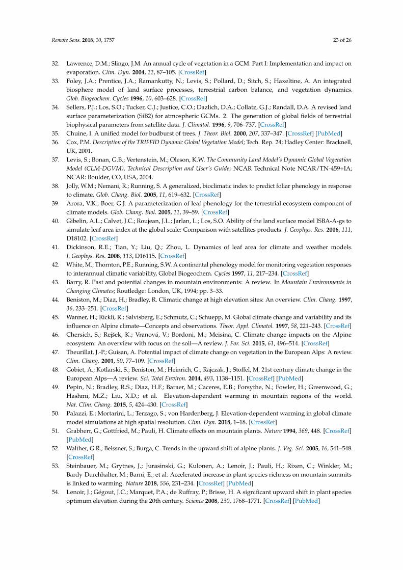
Remote Sens. 2018, 10, 1757 23 of 26

32. Lawrence, D.M.; Slingo, J.M. An annual cycle of vegetation in a GCM. Part I: Implementation and impact onevaporation. Clim. Dyn. 2004, 22, 87–105. [CrossRef]

33. Foley, J.A.; Prentice, J.A.; Ramankutty, N.; Levis, S.; Pollard, D.; Sitch, S.; Haxeltine, A. An integratedbiosphere model of land surface processes, terrestrial carbon balance, and vegetation dynamics.Glob. Biogeochem. Cycles 1996, 10, 603–628. [CrossRef]

34. Sellers, P.J.; Los, S.O.; Tucker, C.J.; Justice, C.O.; Dazlich, D.A.; Collatz, G.J.; Randall, D.A. A revised landsurface parameterization (SiB2) for atmospheric GCMs. 2. The generation of global fields of terrestrialbiophysical parameters from satellite data. J. Climatol. 1996, 9, 706–737. [CrossRef]

35. Chuine, I. A unified model for budburst of trees. J. Theor. Biol. 2000, 207, 337–347. [CrossRef] [PubMed]36. Cox, P.M. Description of the TRIFFID Dynamic Global Vegetation Model; Tech. Rep. 24; Hadley Center: Bracknell,

UK, 2001.37. Levis, S.; Bonan, G.B.; Vertenstein, M.; Oleson, K.W. The Community Land Model’s Dynamic Global Vegetation

Model (CLM-DGVM), Technical Description and User’s Guide; NCAR Technical Note NCAR/TN-459+IA;NCAR: Boulder, CO, USA, 2004.

38. Jolly, W.M.; Nemani, R.; Running, S. A generalized, bioclimatic index to predict foliar phenology in responseto climate. Glob. Chang. Biol. 2005, 11, 619–632. [CrossRef]

39. Arora, V.K.; Boer, G.J. A parameterization of leaf phenology for the terrestrial ecosystem component ofclimate models. Glob. Chang. Biol. 2005, 11, 39–59. [CrossRef]

40. Gibelin, A.L.; Calvet, J.C.; Roujean, J.L.; Jarlan, L.; Los, S.O. Ability of the land surface model ISBA-A-gs tosimulate leaf area index at the global scale: Comparison with satellites products. J. Geophys. Res. 2006, 111,D18102. [CrossRef]

41. Dickinson, R.E.; Tian, Y.; Liu, Q.; Zhou, L. Dynamics of leaf area for climate and weather models.J. Geophys. Res. 2008, 113, D16115. [CrossRef]

42. White, M.; Thornton, P.E.; Running, S.W. A continental phenology model for monitoring vegetation responsesto interannual climatic variability, Global Biogeochem. Cycles 1997, 11, 217–234. [CrossRef]

43. Barry, R. Past and potential changes in mountain environments: A review. In Mountain Environments inChanging Climates; Routledge: London, UK, 1994; pp. 3–33.

44. Beniston, M.; Diaz, H.; Bradley, R. Climatic change at high elevation sites: An overview. Clim. Chang. 1997,36, 233–251. [CrossRef]

45. Wanner, H.; Rickli, R.; Salvisberg, E.; Schmutz, C.; Schuepp, M. Global climate change and variability and itsinfluence on Alpine climate—Concepts and observations. Theor. Appl. Climatol. 1997, 58, 221–243. [CrossRef]

46. Chersich, S.; Rejšek, K.; Vranová, V.; Bordoni, M.; Meisina, C. Climate change impacts on the Alpineecosystem: An overview with focus on the soil—A review. J. For. Sci. 2015, 61, 496–514. [CrossRef]

47. Theurillat, J.-P.; Guisan, A. Potential impact of climate change on vegetation in the European Alps: A review.Clim. Chang. 2001, 50, 77–109. [CrossRef]

48. Gobiet, A.; Kotlarski, S.; Beniston, M.; Heinrich, G.; Rajczak, J.; Stoffel, M. 21st century climate change in theEuropean Alps—A review. Sci. Total Environ. 2014, 493, 1138–1151. [CrossRef] [PubMed]

49. Pepin, N.; Bradley, R.S.; Diaz, H.F.; Baraer, M.; Caceres, E.B.; Forsythe, N.; Fowler, H.; Greenwood, G.;Hashmi, M.Z.; Liu, X.D.; et al. Elevation-dependent warming in mountain regions of the world.Nat. Clim. Chang. 2015, 5, 424–430. [CrossRef]

50. Palazzi, E.; Mortarini, L.; Terzago, S.; von Hardenberg, J. Elevation-dependent warming in global climatemodel simulations at high spatial resolution. Clim. Dyn. 2018, 1–18. [CrossRef]

51. Grabherr, G.; Gottfried, M.; Pauli, H. Climate effects on mountain plants. Nature 1994, 369, 448. [CrossRef][PubMed]

52. Walther, G.R.; Beissner, S.; Burga, C. Trends in the upward shift of alpine plants. J. Veg. Sci. 2005, 16, 541–548.[CrossRef]

53. Steinbauer, M.; Grytnes, J.; Jurasinski, G.; Kulonen, A.; Lenoir, J.; Pauli, H.; Rixen, C.; Winkler, M.;Bardy-Durchhalter, M.; Barni, E.; et al. Accelerated increase in plant species richness on mountain summitsis linked to warming. Nature 2018, 556, 231–234. [CrossRef] [PubMed]

54. Lenoir, J.; Gégout, J.C.; Marquet, P.A.; de Ruffray, P.; Brisse, H. A significant upward shift in plant speciesoptimum elevation during the 20th century. Science 2008, 230, 1768–1771. [CrossRef] [PubMed]

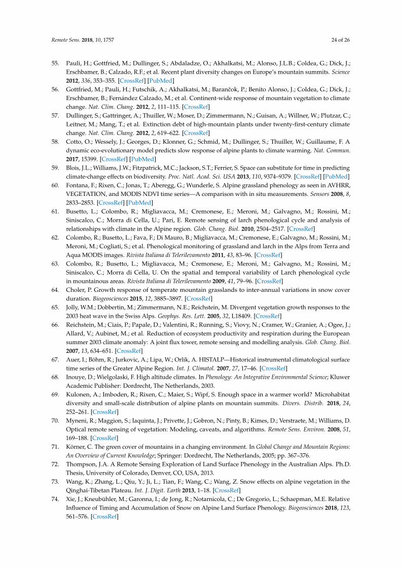
Remote Sens. 2018, 10, 1757 24 of 26

55. Pauli, H.; Gottfried, M.; Dullinger, S.; Abdaladze, O.; Akhalkatsi, M.; Alonso, J.L.B.; Coldea, G.; Dick, J.;Erschbamer, B.; Calzado, R.F.; et al. Recent plant diversity changes on Europe’s mountain summits. Science2012, 336, 353–355. [CrossRef] [PubMed]

56. Gottfried, M.; Pauli, H.; Futschik, A.; Akhalkatsi, M.; Barancok, P.; Benito Alonso, J.; Coldea, G.; Dick, J.;Erschbamer, B.; Fernández Calzado, M.; et al. Continent-wide response of mountain vegetation to climatechange. Nat. Clim. Chang. 2012, 2, 111–115. [CrossRef]

57. Dullinger, S.; Gattringer, A.; Thuiller, W.; Moser, D.; Zimmermann, N.; Guisan, A.; Willner, W.; Plutzar, C.;Leitner, M.; Mang, T.; et al. Extinction debt of high-mountain plants under twenty-first-century climatechange. Nat. Clim. Chang. 2012, 2, 619–622. [CrossRef]

58. Cotto, O.; Wessely, J.; Georges, D.; Klonner, G.; Schmid, M.; Dullinger, S.; Thuiller, W.; Guillaume, F. Adynamic eco-evolutionary model predicts slow response of alpine plants to climate warming. Nat. Commun.2017, 15399. [CrossRef] [PubMed]

59. Blois, J.L.; Williams, J.W.; Fitzpatrick, M.C.; Jackson, S.T.; Ferrier, S. Space can substitute for time in predictingclimate-change effects on biodiversity. Proc. Natl. Acad. Sci. USA 2013, 110, 9374–9379. [CrossRef] [PubMed]

60. Fontana, F.; Rixen, C.; Jonas, T.; Aberegg, G.; Wunderle, S. Alpine grassland phenology as seen in AVHRR,VEGETATION, and MODIS NDVI time series—A comparison with in situ measurements. Sensors 2008, 8,2833–2853. [CrossRef] [PubMed]

61. Busetto, L.; Colombo, R.; Migliavacca, M.; Cremonese, E.; Meroni, M.; Galvagno, M.; Rossini, M.;Siniscalco, C.; Morra di Cella, U.; Pari, E. Remote sensing of larch phenological cycle and analysis ofrelationships with climate in the Alpine region. Glob. Chang. Biol. 2010, 2504–2517. [CrossRef]

62. Colombo, R.; Busetto, L.; Fava, F.; Di Mauro, B.; Migliavacca, M.; Cremonese, E.; Galvagno, M.; Rossini, M.;Meroni, M.; Cogliati, S.; et al. Phenological monitoring of grassland and larch in the Alps from Terra andAqua MODIS images. Rivista Italiana di Telerilevamento 2011, 43, 83–96. [CrossRef]

63. Colombo, R.; Busetto, L.; Migliavacca, M.; Cremonese, E.; Meroni, M.; Galvagno, M.; Rossini, M.;Siniscalco, C.; Morra di Cella, U. On the spatial and temporal variability of Larch phenological cyclein mountainous areas. Rivista Italiana di Telerilevamento 2009, 41, 79–96. [CrossRef]

64. Choler, P. Growth response of temperate mountain grasslands to inter-annual variations in snow coverduration. Biogeosciences 2015, 12, 3885–3897. [CrossRef]

65. Jolly, W.M.; Dobbertin, M.; Zimmermann, N.E.; Reichstein, M. Divergent vegetation growth responses to the2003 heat wave in the Swiss Alps. Geophys. Res. Lett. 2005, 32, L18409. [CrossRef]

66. Reichstein, M.; Ciais, P.; Papale, D.; Valentini, R.; Running, S.; Viovy, N.; Cramer, W.; Granier, A.; Ogee, J.;Allard, V.; Aubinet, M.; et al. Reduction of ecosystem productivity and respiration during the Europeansummer 2003 climate anomaly: A joint flux tower, remote sensing and modelling analysis. Glob. Chang. Biol.2007, 13, 634–651. [CrossRef]

67. Auer, I.; Böhm, R.; Jurkovic, A.; Lipa, W.; Orlik, A. HISTALP—Historical instrumental climatological surfacetime series of the Greater Alpine Region. Int. J. Climatol. 2007, 27, 17–46. [CrossRef]

68. Inouye, D.; Wielgolaski, F. High altitude climates. In Phenology: An Integrative Environmental Science; KluwerAcademic Publisher: Dordrecht, The Netherlands, 2003.

69. Kulonen, A.; Imboden, R.; Rixen, C.; Maier, S.; Wipf, S. Enough space in a warmer world? Microhabitatdiversity and small-scale distribution of alpine plants on mountain summits. Divers. Distrib. 2018, 24,252–261. [CrossRef]

70. Myneni, R.; Maggion, S.; Iaquinta, J.; Privette, J.; Gobron, N.; Pinty, B.; Kimes, D.; Verstraete, M.; Williams, D.Optical remote sensing of vegetation: Modeling, caveats, and algorithms. Remote Sens. Environ. 2008, 51,169–188. [CrossRef]

71. Körner, C. The green cover of mountains in a changing environment. In Global Change and Mountain Regions:An Overview of Current Knowledge; Springer: Dordrecht, The Netherlands, 2005; pp. 367–376.

72. Thompson, J.A. A Remote Sensing Exploration of Land Surface Phenology in the Australian Alps. Ph.D.Thesis, University of Colorado, Denver, CO, USA, 2013.

73. Wang, K.; Zhang, L.; Qiu, Y.; Ji, L.; Tian, F.; Wang, C.; Wang, Z. Snow effects on alpine vegetation in theQinghai-Tibetan Plateau. Int. J. Digit. Earth 2013, 1–18. [CrossRef]

74. Xie, J.; Kneubühler, M.; Garonna, I.; de Jong, R.; Notarnicola, C.; De Gregorio, L.; Schaepman, M.E. RelativeInfluence of Timing and Accumulation of Snow on Alpine Land Surface Phenology. Biogeosciences 2018, 123,561–576. [CrossRef]

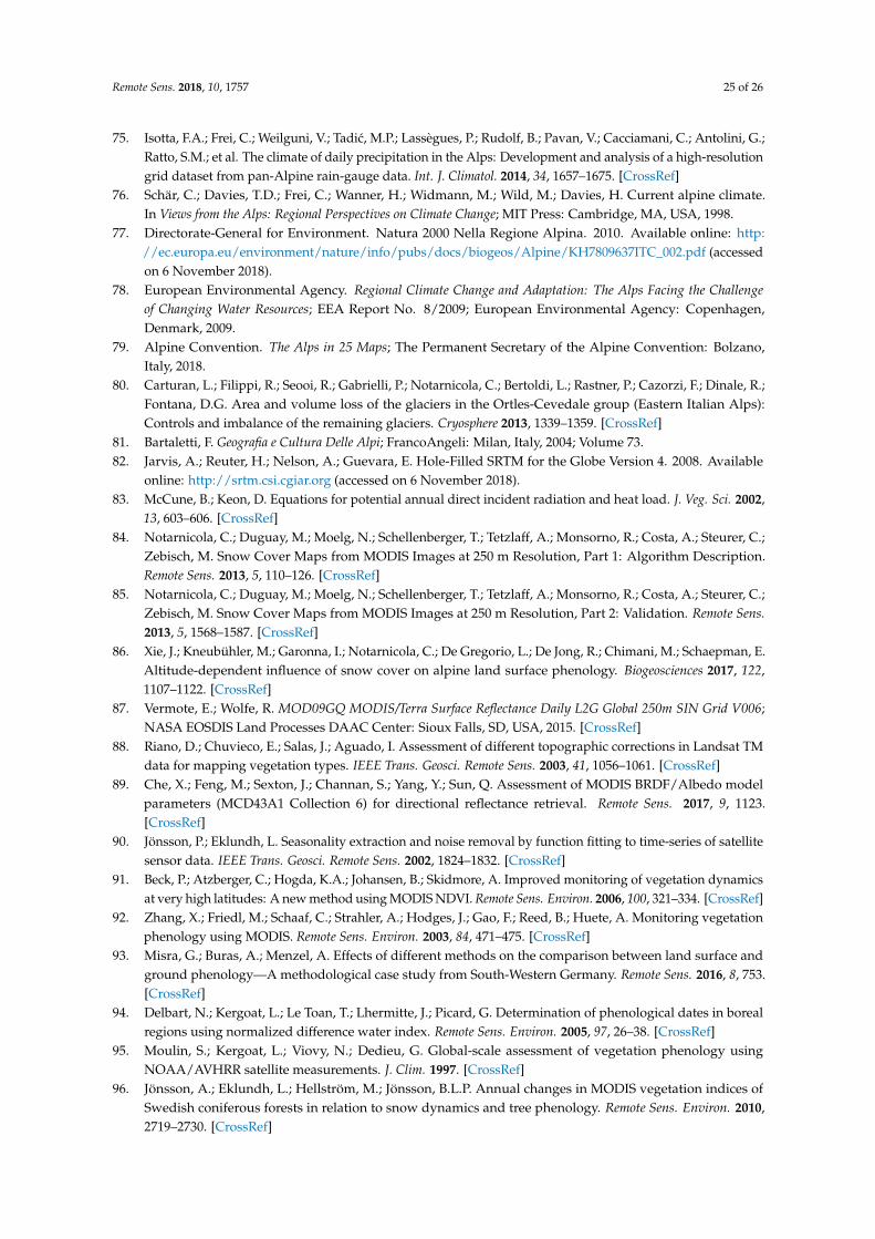
Remote Sens. 2018, 10, 1757 25 of 26

75. Isotta, F.A.; Frei, C.; Weilguni, V.; Tadic, M.P.; Lassègues, P.; Rudolf, B.; Pavan, V.; Cacciamani, C.; Antolini, G.;Ratto, S.M.; et al. The climate of daily precipitation in the Alps: Development and analysis of a high-resolutiongrid dataset from pan-Alpine rain-gauge data. Int. J. Climatol. 2014, 34, 1657–1675. [CrossRef]

76. Schär, C.; Davies, T.D.; Frei, C.; Wanner, H.; Widmann, M.; Wild, M.; Davies, H. Current alpine climate.In Views from the Alps: Regional Perspectives on Climate Change; MIT Press: Cambridge, MA, USA, 1998.

77. Directorate-General for Environment. Natura 2000 Nella Regione Alpina. 2010. Available online: http://ec.europa.eu/environment/nature/info/pubs/docs/biogeos/Alpine/KH7809637ITC_002.pdf (accessedon 6 November 2018).

78. European Environmental Agency. Regional Climate Change and Adaptation: The Alps Facing the Challengeof Changing Water Resources; EEA Report No. 8/2009; European Environmental Agency: Copenhagen,Denmark, 2009.

79. Alpine Convention. The Alps in 25 Maps; The Permanent Secretary of the Alpine Convention: Bolzano,Italy, 2018.

80. Carturan, L.; Filippi, R.; Seooi, R.; Gabrielli, P.; Notarnicola, C.; Bertoldi, L.; Rastner, P.; Cazorzi, F.; Dinale, R.;Fontana, D.G. Area and volume loss of the glaciers in the Ortles-Cevedale group (Eastern Italian Alps):Controls and imbalance of the remaining glaciers. Cryosphere 2013, 1339–1359. [CrossRef]

81. Bartaletti, F. Geografia e Cultura Delle Alpi; FrancoAngeli: Milan, Italy, 2004; Volume 73.82. Jarvis, A.; Reuter, H.; Nelson, A.; Guevara, E. Hole-Filled SRTM for the Globe Version 4. 2008. Available

online: http://srtm.csi.cgiar.org (accessed on 6 November 2018).83. McCune, B.; Keon, D. Equations for potential annual direct incident radiation and heat load. J. Veg. Sci. 2002,

13, 603–606. [CrossRef]84. Notarnicola, C.; Duguay, M.; Moelg, N.; Schellenberger, T.; Tetzlaff, A.; Monsorno, R.; Costa, A.; Steurer, C.;

Zebisch, M. Snow Cover Maps from MODIS Images at 250 m Resolution, Part 1: Algorithm Description.Remote Sens. 2013, 5, 110–126. [CrossRef]

85. Notarnicola, C.; Duguay, M.; Moelg, N.; Schellenberger, T.; Tetzlaff, A.; Monsorno, R.; Costa, A.; Steurer, C.;Zebisch, M. Snow Cover Maps from MODIS Images at 250 m Resolution, Part 2: Validation. Remote Sens.2013, 5, 1568–1587. [CrossRef]

86. Xie, J.; Kneubühler, M.; Garonna, I.; Notarnicola, C.; De Gregorio, L.; De Jong, R.; Chimani, M.; Schaepman, E.Altitude-dependent influence of snow cover on alpine land surface phenology. Biogeosciences 2017, 122,1107–1122. [CrossRef]

87. Vermote, E.; Wolfe, R. MOD09GQ MODIS/Terra Surface Reflectance Daily L2G Global 250m SIN Grid V006;NASA EOSDIS Land Processes DAAC Center: Sioux Falls, SD, USA, 2015. [CrossRef]

88. Riano, D.; Chuvieco, E.; Salas, J.; Aguado, I. Assessment of different topographic corrections in Landsat TMdata for mapping vegetation types. IEEE Trans. Geosci. Remote Sens. 2003, 41, 1056–1061. [CrossRef]

89. Che, X.; Feng, M.; Sexton, J.; Channan, S.; Yang, Y.; Sun, Q. Assessment of MODIS BRDF/Albedo modelparameters (MCD43A1 Collection 6) for directional reflectance retrieval. Remote Sens. 2017, 9, 1123.[CrossRef]

90. Jönsson, P.; Eklundh, L. Seasonality extraction and noise removal by function fitting to time-series of satellitesensor data. IEEE Trans. Geosci. Remote Sens. 2002, 1824–1832. [CrossRef]

91. Beck, P.; Atzberger, C.; Hogda, K.A.; Johansen, B.; Skidmore, A. Improved monitoring of vegetation dynamicsat very high latitudes: A new method using MODIS NDVI. Remote Sens. Environ. 2006, 100, 321–334. [CrossRef]

92. Zhang, X.; Friedl, M.; Schaaf, C.; Strahler, A.; Hodges, J.; Gao, F.; Reed, B.; Huete, A. Monitoring vegetationphenology using MODIS. Remote Sens. Environ. 2003, 84, 471–475. [CrossRef]

93. Misra, G.; Buras, A.; Menzel, A. Effects of different methods on the comparison between land surface andground phenology—A methodological case study from South-Western Germany. Remote Sens. 2016, 8, 753.[CrossRef]

94. Delbart, N.; Kergoat, L.; Le Toan, T.; Lhermitte, J.; Picard, G. Determination of phenological dates in borealregions using normalized difference water index. Remote Sens. Environ. 2005, 97, 26–38. [CrossRef]

95. Moulin, S.; Kergoat, L.; Viovy, N.; Dedieu, G. Global-scale assessment of vegetation phenology usingNOAA/AVHRR satellite measurements. J. Clim. 1997. [CrossRef]

96. Jönsson, A.; Eklundh, L.; Hellström, M.; Jönsson, B.L.P. Annual changes in MODIS vegetation indices ofSwedish coniferous forests in relation to snow dynamics and tree phenology. Remote Sens. Environ. 2010,2719–2730. [CrossRef]

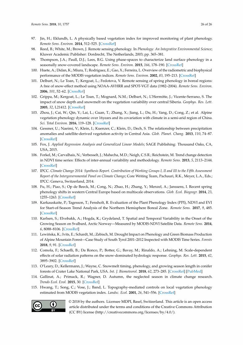
Remote Sens. 2018, 10, 1757 26 of 26

97. Jin, H.; Eklundh, L. A physically based vegetation index for improved monitoring of plant phenology.Remote Sens. Environ. 2014, 512–525. [CrossRef]

98. Reed, B.; White, M.; Brown, J. Remote sensing phenology. In Phenology: An Integrative Environmental Science;Kluwer Academic Publisher: Dordrecht, The Netherlands, 2003; pp. 365–381.

99. Thompson, J.A.; Paull, D.J.; Lees, B.G. Using phase-spaces to characterize land surface phenology in aseasonally snow-covered landscape. Remote Sens. Environ. 2015, 166, 178–190. [CrossRef]

100. Huete, A.; Didan, K.; Miura, T.; Rodriguez, E.; Gao, X.; Ferreira, L. Overview of the radiometric and biophysicalperformance of the MODIS vegetation indices. Remote Sens. Environ. 2002, 83, 195–213. [CrossRef]

101. Delbart, N.; Le Toan, T.; Kergoat, L.; Fedotova, V. Remote sensing of spring phenology in boreal regions:A free of snow-effect method using NOAA-AVHRR and SPOT-VGT data (1982–2004). Remote Sens. Environ.2006, 101, 52–62. [CrossRef]

102. Grippa, M.; Kergoat, L.; Le Toan, T.; Mognard, N.M.; Delbart, N.; L’Hermitte, J.; Vicente-Serrano, S. Theimpact of snow depth and snowmelt on the vegetation variability over central Siberia. Geophys. Res. Lett.2005, 32, L21412. [CrossRef]

103. Zhou, J.; Cai, W.; Qin, Y.; Lai, L.; Guan, T.; Zhang, X.; Jiang, L.; Du, H.; Yang, D.; Cong, Z.; et al. Alpinevegetation phenology dynamic over 16years and its covariation with climate in a semi-arid region of China.Sci. Total Environ. 2016, 119–128. [CrossRef]

104. Gessner, U.; Naeimi, V.; Klein, I.; Kuenzer, C.; Klein, D.; Dech, S. The relationship between precipitationanomalies and satellite-derived vegetation activity in Central Asia. Glob. Planet. Chang. 2013, 110, 74–87.[CrossRef]

105. Fox, J. Applied Regression Analysis and Generalized Linear Models; SAGE Publishing: Thousand Oaks, CA,USA, 2015.

106. Forkel, M.; Carvalhais, N.; Verbesselt, J.; Mahecha, M.D.; Neigh, C.S.R.; Reichstein, M. Trend change detectionin NDVI time series: Effects of inter-annual variability and methodology. Remote Sens. 2013, 5, 2113–2144.[CrossRef]

107. IPCC. Climate Change 2014: Synthesis Report. Contribution of Working Groups I, II and III to the Fifth AssessmentReport of the Intergovernmental Panel on Climate Change; Core Writing Team, Pachauri, R.K., Meyer, L.A., Eds.;IPCC: Geneva, Switzerland, 2014.

108. Fu, H.; Piao, S.; Op de Beeck, M.; Cong, N.; Zhao, H.; Zhang, Y.; Menzel, A.; Janssens, I. Recent springphenology shifts in western Central Europe based on multiscale observations. Glob. Ecol. Biogeogr. 2014, 23,1255–1263. [CrossRef]

109. Karkauskaite, P.; Tagesson, T.; Fensholt, R. Evaluation of the Plant Phenology Index (PPI), NDVI and EVIfor Start-of-Season Trend Analysis of the Northern Hemisphere Boreal Zone. Remote Sens. 2017, 9, 485.[CrossRef]

110. Karlsen, S.; Elvebakk, A.; Hogda, K.; Grydeland, T. Spatial and Temporal Variability in the Onset of theGrowing Season on Svalbard, Arctic Norway—Measured by MODIS-NDVI Satellite Data. Remote Sens. 2014,6, 8088–8106. [CrossRef]

111. Lewinska, K.; Ivits, E.; Schardt, M.; Zebisch, M. Drought Impact on Phenology and Green Biomass Productionof Alpine Mountain Forest—Case Study of South Tyrol 2001–2012 Inspected with MODIS Time Series. Forests2018, 9, 91. [CrossRef]

112. Comola, F.; Schaefli, B.; Da Ronco, P.; Botter, G.; Bavay, M.; Rinaldo, A.; Lehning, M. Scale-dependenteffects of solar radiation patterns on the snow-dominated hydrologic response. Geophys. Res. Lett. 2015, 42,3895–3902. [CrossRef]

113. O’Leary, D.; Kellermann, J.; Wayne, C. Snowmelt timing, phenology, and growing season length in coniferforests of Crater Lake National Park, USA. Int. J. Biometeorol. 2018, 62, 273–285. [CrossRef] [PubMed]

114. Gallinat, A.; Primack, R.; Wagner, D. Autumn, the neglected season in climate change research.Trends Ecol. Evol. 2015, 30. [CrossRef]

115. Hwang, T.; Song, C.; Vose, J.; Band, L. Topography-mediated controls on local vegetation phenologyestimated from MODIS vegetation index. Landsc. Ecol. 2001, 26, 541–556. [CrossRef]

© 2018 by the authors. Licensee MDPI, Basel, Switzerland. This article is an open accessarticle distributed under the terms and conditions of the Creative Commons Attribution(CC BY) license (http://creativecommons.org/licenses/by/4.0/).