Download pdf - Scheduling in Systems with Indeterminate Processing Times

www.as-se.org/sss Studies in System Science (SSS) Volume 1 Issue 3, September 2013

50

Scheduling in Systems with Indeterminate Processing Times Vitaly I. Levin

Mathematics Department, Penza State Technological University 1-a, Baidukov pr., Penza, 440039, Russia [email protected]

Abstract

A general approach to the synthesis of an optimal order of executing jobs in engineering systems with indeterminate (interval) times of job processing is presented. As a mathematical model of the system, a two-stage pipeline is taken whose first and second stages are, respectively, the input of data and its processing, and the corresponding mathematical apparatus is continuous logic and logic determinants.

Keywords

Continuous Logic; System; Optimal Order of Jobs

Introduction

The study of systems begins with determining the dependence of the performance factor of the system on its various parameters. This dependence can be used to estimate the performance factor of system, to analyze it qualitatively, to optimally synthesize the system, etc. As a rule, the existing estimation methods for performance of systems are oriented only to calculating performance factor of system but are not meant for their analysis and synthesis [Drummond].

In [Levin, 2011 a] there is an approach to studsystems based on pipeline model of scheduling theory and on mathematical apparatus of continuous logic and logical determinants, which makes it possible to derive an observable and easily calculated expression for system performance and to carry out qualitative analysis of effect of system parameters on its performance and optimal synthesis according to the criterion of best performance. In this case, the time parameters are assumed to be deterministic. In practice, these parameters are in many cases nondeterministic, which substantially hampers the study of the system.

An extension of the general approach has been taken into account for optimal synthesis of various type systems with uncertain (interval) type time parameters to nondeterministic case [Levin, 2011 a]. Under

application of this approach to optimal synthesis of systems with interval time parameters, this common problem reduces to solving similar problems for two systems with deterministic time parameters equal to the upper and lower bounds of the corresponding intervals.

Problem Statement

Consider an engineering system operating in a batch mode and let the batch contain n different jobs 1,2,...,n , and then employ the simplest two-phase model of the system. So, in the first phase performed by the first system unit the first operation, namely the input of the initial data, is carried out; further, in other phase performed by the second system unit, the second operation is carried out:transformation and processing of these data in the various functional units of the system (processor, main memory, and external memory) and the output the result. The units are assumed to operate consecutively. Each job ( 1, )i i n= firstly goes to the first system unit, where first operation is full performed, and after that it goes to the second unit, where the second operation is carried out completely.

The time of execution of the first operation on arbitrary job i is assumed to be known inexactly and to be determined by a closed interval 1 2[ , ]i i ia a a= of all possible values of this time. In similar way, the time of execution of the second operation on job i is set:

1 2[ , ]i i ib b b= . Therefore, the first unit starts the execution of the current job immediately after the end of the previous job, i.e., it operates without idle times, whereas the second unit starts the execution of the current job j only after the job j leaves the first unit, i.e., in the general case, it operates with idle times. It is required to choose an order of jobs in the system under which its best performance is ensured, i.e., total execution time of all jobs is minimum.

As in determiniscic case [Johnson, Muth], the optimal

Studies in System Science (SSS) Volume 1 Issue 3, September 2013 www.as-se.org/sss

51

order of jobs can be assumed to be permutable, i.e., jobs must pass through two units in same order. Assume that execution times of first and second operations on an arbitrary job i are exact and equal to

ia and ib , respectively. Let for a pair of jobs ( , )i j the order of passage through the first unit be i j→ , and the order of passage through second unit be in opposition: j i→ . Let us change the order of jobs passing in the first unit by placing job i after j and moving job j (together with the jobs located earlier between i and j ) to the left by length of freed time interval ia . In this case, the interval of execution of one of the jobs i which are subject to permutation, is moved to the right. However, it then ends at the time of completion of the execution of the job j in the first unit (before permutation, i.e., as previously, before the time of beginning of the execution of the job in the second unit). Hence, a change in the order of jobs in the first unit does not affect the sequence of jobs in the second unit. Therefore, the same order of passage of jobs through the two units can be chosen without changing the resultant time of execution of all jobs. It means that for deterministic execution times of operations the optimal order in the sequence of jobs passing can be sought within the set of permutational orders of jobs. This conclusion is true for arbitrary deterministic execution times ia and ib of operations inside the given interval values 1 2[ , ]i i ia a a= and

1 2[ , ]i i ib b b= . Consequently, in accordance with the conditions of the problem, it remains valid if times of operations are assumed to be equal to the indicated interval values.

Thus, the solution of the stated problem reduces to finding an external permutation

1 2( , ,.., ), {1,2,..., }n n kP i i i i n= ∈ , (1) of n given jobs that determines the order of jobs in the system, which is the same for its two units. The symbol ki in expression (1) is the index of the job occupying the k -th place in the ordered sequence.

Logic Algebra of Nondeterministic Quantities and Their Comparison

The problem solution requires some facts of the logic of nondeterministic interval quantities and of comparison theory for these quantities [Levin, 2012]. We shall proceed from continuous logic for deterministic (point) quantities [Levin, 2011 b]. Basic logical operations on these points are disjunction ∨ and conjunction ∧ that are defined in following formulas:

max( , ), min( , )a b a b a b a b∨ = ∧ = . (2) Here ,a b C∈ , and the set C is an arbitrary interval of real numbers. Operations (2) obey the majority of laws of discrete logic, namely

,a a aa a a∨ =∧ =

(tautology) (3)

,a b b aa b b a∨ = ∨∧ = ∧

(commutative law) (4)

( ) ( ),( ) ( )a b c a b ca b c a b c∨ ∨ = ∨ ∨∧ ∧ = ∧ ∧

(associative law) (5)

( ) ( ) ( ),( ) ( ) ( )

a b c a b a ca b c a b a c∨ ∧ = ∨ ∧ ∨∧ ∨ = ∧ ∨ ∧

(distributive law)(6)

( ) , ( )a a b a a a b a∨ ∧ = ∧ ∨ = (7)

( ) ( ) ( )a b c a b a c∨ ∨+ = + +∧ ∧

, (8)

( ) ( ) ( )a b c a b a c∨ ∧− = − −∧ ∨

, (9)

( ) ( ) ( ), , , 0a b c a b a c a b c∨ ∨= >∧ ∧

⋅ ⋅ ⋅ , (10)

( ) ( ) ( ), , , 0a b c a b a c a b c∨ ∧− = − − >∧ ∨

⋅ ⋅ ⋅ , (11)

A special partial case of the equation (11) for 1a = is the following law:

( ) ( ) ( )b c b c∨ ∧− = − −∧ ∨

, (12)

We now pass to continuous logic for interval quantities. In this case, the continuous-logical operations of disjunction and conjunction (2) are generalized as set-theoretic constructions:

{ | , };{ | , }.

a b a b a a b ba b a b a a b b∨ = ∨ ∈ ∈

∧ = ∧ ∈ ∈

(13)

Here 1 2[ , ]a a a= and 1 2[ , ]b b b= are intervals regarded as the corresponding sets of points (values) belonging to them. According to [Levin, 2012], operations on intervals (13) obey the same laws (3)–(12) as the operations on point quantities (2). In particular, distributive laws (8) and the law (12) take form:

( ) ( ) ( )a b c a b a c∨ ∨+ = + +∧ ∧

, (14)

( ) ( ) ( )b c b c∨ ∧− = − −∧ ∨

. (15)

Due to [Levin, 2012] the results of the logical operations of disjunction and conjunction on intervals (13) are calculated by the formulas

1 2 1 2 1 1 2 2[ , ] [ , ] [ , ],a b a a b b a b a b∨ = ∨ = ∨ ∨ (16)

1 2 1 2 1 1 2 2[ , ] [ , ] [ , ],a b a a b b a b a b∧ = ∧ = ∧ ∧ (17) Some important facts of comparison theory for intervals are briefly presented [Levin, 2012].

1. For any pair of intervals 1 2[ , ]a a a= and 1 2[ , ]b b b= the equivalence relation

( ) ( )a b a a b b∨ = ⇔ ∧ = , (18)


52

holds, i.e., like point quantities, the intervals are compatible (in the sense that if one of the two quantities is maximal, then the other is minimal and vice versa).

2. Pairs of intervals 1 2[ , ]a a a= and 1 2[ , ]b b b= can be in relations ”greater than” and ”smaller than” defined in the same way as in the case of point quantities by the such equivalence:

( ) ( , )a b a b a a b b≥ ⇔ ∨ = ∧ = . (19)

3. In accordance with (19), any two intervals a and b that are in relation a b≥ or a b≤ are said to be comparable. Otherwise a and b are incomparable.

4. For intervals 1 2[ , ]a a a= and 1 2[ , ]b b b= to be comparable and satisfying the relation a b≥ it is necessary and sufficient that the system of inequalities

1 1 2 2( , )a b a b≥ ≥ holds, and for a and b to be incomparable it is necessary and sufficient that at least one of the systems of inequalities 1 1 2 2( , )a b a b< > or

1 1 2 2( , )b a b a< > is true. Thus, only the intervals displaced relative to each other along the number axis are comparable; in this case the interval displaced to the right is greater. If one of intervals overlaps the other, the intervals are incomparable.

5. In a system of intervals 1 2, ,..., ka a a the interval 1a is said to be maximal (minimal) interval if it is comparable with other intervals 2 ,..., ka a and in the relations 1 2 1,..., ka a a a≥ ≥ 1 2 1( ,..., )ka a a a≤ ≤ with them.

6. It is necessary and sufficient for interval 1a in system of intervals 1 11 12 2 21 22[ , ], [ , ],...,a a a a a a= = 1 2[ , ]k k ka a a= be maximal that the system of the relations holds:

11 1 12 21 1

,k k

i ii i

a a a a= =

= =∨ ∨ , (20)

and for 1a to be minimal it is necessary and sufficient that following equations is true:

11 1 12 21 1

,k k

i ii i

a a a a= =

= =∧ ∧ , (21)

Derivation of Optimality Conditions

In previous case, a relationship has been defined between the execution times , , ,i i j ja b a b of two arbitrary jobs ( , )i j under which they must be executed in order i j→ in optimal sequence of jobs ( )P n (1). Let

1( ,..., );k kP i i k n= ≤ , be initial section of nP and 1( )kt P and

2( )kt P be the time intervals containing all possible time instants of completion of the sequence kP in first and second units. Because 1 1( , )k k kP P i+ += , we can write

1

1

1 1

2 1 1 1

( ) ( ) ,

( ) [ ( ) ( )] .k

k

k k i

k k k i

t P t P a

t P t P t P b+

+

+

+ +

= +

= ∨ +

(22)

Here ∨ is disjunction of type (13). The recurrence relations (22) make it possible to calculate the total time of execution for any order of the sequence of jobs

nP in the form of a time interval 2(2, ) ( ).nT n t P=

Let 11 1( ,..., , , ,..., )n k nP i i i j j= and 2

1 1( ,..., , , ,..., )n k nP i i j j j= be two sequences of jobs passing through the system that differ only in the order of execution of jobs i and j occupying the ( 1)k + -th and ( 2)k + -th positions in the sequence. Let us find out when 1

nP is more preferable than 2

nP , i.e. when jobs i and j must be executed in order i j→ (and not vice versa). The corresponding condition is written as

1 22 2 2 2( ) ( )k kt P t P+ +≤ . (23)

According to (22), the sequence 1nP is more preferable

than 2nP if the time or passage of its regulated

subsequence 12kP + through two units is less than that of

22kP + . To write preference condition in explicit form, we

must express 2 2( )kt P + via the time parameters ia and ib

of jobs. Let 1( )kt P t= . Then 2( )kt P t= + ∆ , where ki

b∆ = .

Due to the fact that 11 ( , )k kP P i+ = and 1 1

2 1( , ) ( , , )k k kP P j P i j+ += = , on applying twice recurrence relations (22) we obtain

1 11 1 2 1

11 2

12 2

( ) ; ( ) (( ) ( )) ;( ) ;

( ) {( ) [(( ) ( )) ]}.

k i k i i

k i j

k i j i i

t P t a t P t a t bt P t a a

t P t a a t a t b

+ +

+

+

= + = + ∨ + ∆ +

= + +

= + + ∨ + ∨ + ∆ +

We similarly determine haracteristics 21kP + and 2

2kP + ; in this case we have

22 2( ) {( ) [(( ) ( )) ]}k i j i j it P t a a t a t b b+ = + + ∨ + ∨ + ∆ + + .

The substitution of the above expressions into the formula (23) yields explicit form of the condition under which the jobs i and j in the optimal sequence must follow in the order i j→ :

{( ) [(( ) ( )) ]}

{( ) [(( ) ( )) ]} .i j i i i

i j j j i

t a a t a t b b

t a a t a t b b

+ + ∨ + ∨ + ∆ + + ≤

≤ + + ∨ + ∨ + ∆ + +

(24)

To simplify inequalities (24) we apply the laws (8), (12) and we can take by (8) the term t outside the parentheses on both sides of (24). On canceling it, we find

{( ) [( ) ]} {( ) [( ) ]}i j i i j i j i j ia a a b b a a a b b+ ∨ ∨ ∆ + + ≤ + ∨ ∨ ∆ + + .

We now take the terms , ,i j ia a b and , ,i j ja a b outside the curly brackets on left- and right-hand sides of the new inequality, respectively. On canceling the common terms on the two sides, we write


53

( ) ( ) ( ) ( ) ( ) ( )i i j j j i j ib a a a b a a a− ∨ ∆ − − ∨ − ≤ − ∨ ∆ − − ∨ − . Based on law (12), we take the minus sign outside all brackets in the last inequality and multiply its left- and right-hand sides by 1− , which results in

( ) ( )i j i j j i i ja b a a a b a a∧ ∧ + − ∆ ≤ ∧ ∧ + − ∆ . (25)

The symbol ∧ in (25) is conjunction (13). Let us solve inequality (25). We rewrite it in the form

L D M D∧ ≤ ∧ , (26) where ,i j j iL a b M a b= ∧ = ∧ , i jD a a= + − ∆ . The logical inequality (26) for interval quantities is solved by same separation method as for point quantities [Levin, 2011 b]. We obtain L M≤ (always), L M> (for )D M≤ for (26), and, on returning to the original quantities, we derive the following solutions to (25):

i j j ia b a b∧ ≤ ∧ , (27)

i j j i i ja a a b a b+ − ∆ ≤ ∧ < ∧ , (28) The inequality (27) involves only time characteristics of jobs i and j . Therefore, if (27) holds then jobs ,i j in the optimal sequence nP follow in the order i j→ irrespective of the order of the other jobs. Besides the characteristics of i and j , inequality (28) contains the parameter ∆ depending on subsequence kP preceding i and j . Fulfillment of condition (28) means that jobs i and j in the optimal sequence nP for execution of jobs follow in order i j→ only in the case when the preceding subsequence kP has the corresponding value of the parameter ∆ . It is clear that for optimal scheduling of jobs it is more advisable to use condition (27) stated as the following independent theorem.

Theorem 1. For jobs i and j in optimal sequence of execution of all n jobs in a two-unit nondetermined system with execution times of first and second operations of job i in form of intervals 1 2[ , ]i i ia a a= and

1 2[ , ]i i ib b b= to follow in the order i j→ irrespective of the order of execution of the other jobs, it is necessary and sufficient that the time parameters i and j satisfy condition (27).

Reduction to Deterministic Problems

We will reduce the optimality conditions for the jobs execution order in non-determined engineering system in question that are established in Theorem 1 to well-known optimality conditions for the order of execution of jobs in different deterministic systems [Johnson, Muth], taking two two-unit deterministic systems into consideration. Let the execution times of the first and second operations on an arbitrary job i in

the first system be equal to the lower bounds 1ia and

1ib of the times ia and ib of execution of these operations in the given nondeterministic system, respectively, and let in other systems these times be equal to the lower and upper bounds 2ia and 2ib of the times ia and ib . We will call these systems the lower and upper deterministic boundary systems relative to the nondeterministic system.

Theorem 2. For jobs i and j in optimal sequence of execution of all n jobs in a two-unit nondetermined system with execution times of first and second operations on job i in form of intervals 1 2[ , ]i i ia a a= and

1 2[ , ]i i ib b b= to be carried out in the order i j→ irrespective of the order of execution of the other jobs, it is necessary and sufficient that jobs i and j should be carried out in same order irrespective of execution of other jobs, i.e. in order of execution in the optimal sequences for execution of all jobs in two deterministic two-unit systems, namely, in lower and upper boundary systems.

Proof. Rewrite first inequality (27) in explicit interval form by substituting corresponding values of intervals into the form: 1 2 1 2 1 2 1 2[ , ] [ , ] [ , ] [ , ]i i j j j j i ia a b b a a b b∧ ≤ ∧ . By (17), on the performing conjunctions of intervals, we obtain

1 1 2 2 1 1 2 2[ , ] [ , ]i j i j j i j ia b a b a b a b∧ ∧ ≤ ∧ ∧ .

According to the rule 4, this inequality for the interval values can be rewritten in the form of an equivalent system of two ordinary inequalities:

1 1 1 1 2 2 2 2, ]i j j i i j j ia b a b a b a b∧ ≤ ∧ ∧ ≤ ∧ .

By the laws of deterministic scheduling theory [4], [6], it can be seen that the first inequality of (29) is a necessary and sufficient condition for jobs i and j in the optimal sequence for execution in two-unit determined systems with times 1ia and 1ib of the first and second operations execution of the jobs i and j carried out in order i j→ irrespective of execution order of the other jobs. Analogically, the second inequality of (29) is a necessary and sufficient condition for jobs i and j in optimal sequence of all jobs execution in the two-unit determined processing system with time parameters 2ia and 2ib of the execution of first and second operations of job i (i.e. in upper boundary system) to be carried out in the order i j→ irrespective of the order of execution of the other jobs.

Further, by the Theorem 1, inequality (27) and consequently inequalities (29) are necessary and


54

sufficient conditions for jobs i and j in optimal sequence of all jobs execution in two-unit nondetermined system with execution parameters

1 2[ , ]i i ia a a= and 1 2[ , ]i i ib b b= . They are intervals of times of the first and second operations of job i to be carried out in the order i j→ irrespective of order of execution of all other jobs. It is the last assertion together with foregoing two assertions that proves completely Theorem 2 which implies following theorem.

Theorem 3. For a type (1) permutation 1( ,..., )n nP i i= being an optimal sequence of the execution of n jobs in a nondeterministic two-unit system with times of execution of the first and second operations of job i in form of the intervals 1 2[ , ]i i ia a a= and 1 2[ , ]i i ib b b= it is necessary and sufficient that nP be also optimal sequence of execution of n operations in lower and upper boundary systems. Theorem 3 implies two theorems below.

Theorem 4. The set M which holds all optimal sequ-ences of n jobs in nondetermined two-unit system with times of execution of the first and second operations of job i in form of intervals 1 2[ , ]i i ia a a= and

1 2[ , ]i i ib b b= is the intersection of the sets lM and uM which content all optimal sequences of n jobs in its lower and upper deterministic boundary systems.

Theorem 5. For the optimal sequence of all implemeted n jobs 1( ,..., )n nP i i= existing in the nondeterministic two-unit system with the execution time parameters of the first and second operations of job i in form of intervals 1 2[ , ]i i ia a a= and 1 2[ , ]i i ib b b= , it is necessary and sufficient that the intersection of lM and uM sets of all optimal sequences of n jobs execution in its lower and upper determined boundary systems are nonempty.

Theorems 4 and 5 imply the following direct solution algorithm for stated problem, i.e. to find an optimal sequence 1( ,..., )n nP i i= of execution of n jobs in a nondeterministic two-unit system with corresponding execution times of first and second operations of job i in the form of intervals 1 2[ , ]i i ia a a= and 1 2[ , ]i i ib b b= .

Step 1. Finding the set lM of all optimal sequences of execution of n jobs in lower boundary system of original system with execution times 1i ia a= and 1i ib b= which are accordingly the times of first and second operations of job i . The well-known solution methods for deterministic two-stage problem of scheduling in

industrial systems are used [Levin, 2011 a, Johnson, Muth].

Step 2. Finding the set uM of all optimal sequences of execution of n jobs in upper boundary system of original system with execution times 2i ia a= and 2i ib b= which are accordingly the times of first and second operations of job i , using the same methods as in Step 1.

Step 3. Finding the intersection l uM M∩ of the sets, which is the set M of all optimal sequences of execution of n jobs in the given nondeterministic two-unit system. If M ≠ ∅ then any sequence nP M∈ is desired optimal sequence of execution of n jobs. If M = ∅ then there are no such sequences.

The suggested direct solution algorithm for the problem requires exhaustion when determining the intersection of the sets lM , uM , and therefore it is efficient only for 1l uM M= = or for lM and uM

close to 1. In case when the value of lM or uM is large, the direct algorithm is ineffective, and it is necessary to pass to application of decision rules making it possible to find an optimal sequence of the implementation of the jobs in the nondeterministic system without exhaustion.

Construction of Decision Rules

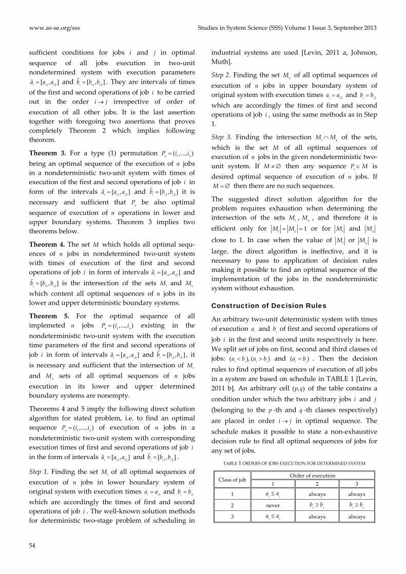
An arbitrary two-unit deterministic system with times of execution ia and ib of first and second operations of job i in the first and second units respectively is here. We split set of jobs on first, second and third classes of jobs: ( ), ( )i i i ia b a b< > and ( )i ia b= . Then the decision rules to find optimal sequences of execution of all jobs in a system are based on schedule in TABLE 1 [Levin, 2011 b]. An arbitrary cell ( )p,q of the table contains a condition under which the two arbitrary jobs i and j (belonging to the p -th and q -th classes respectively) are placed in order i j→ in optimal sequence. The schedule makes it possible to state a non-exhaustive decision rule to find all optimal sequences of jobs for any set of jobs.

TABLE 1 ORDERS OF JOBS EXECUTION FOR DETERMINED SYSTEM

Class of job Order of execution

1 2 3

1 i ja a≤ always always

2 never i jb b≥ i jb b≥

3 i ja a≤ always always


55

The cell (1 1), , for example, shows that for the set of jobs of the first class, the optimal execution sequence is obtained by arrangment of i jobs in the increasing (nondecreasing) order relative to parameter ia [Levin, 2011 b].

Let us apply a similar approach to optimize a given nondeterministic two-unit system with execution times of the first and second operations of job i in form of intervals 1 2[ , ]i i ia a a= and 1 2[ , ]i i ib b b= . Along with this system, considering its lower and upper deterministic boundary processing systems (Table 1), the former has execution times 1ia and 1ib of the 1st and 2nd operations of job i , and for the latter one, these values are 2ia and 2ib . By Theorem 3, an optimal sequence of execution of jobs in a nondeterministic system is also an optimal sequence of the execution of jobs in its lower and upper deterministic boundary systems. Therefore, the optimality condition for a sequence of jobs in a nondeterministic system is the intersection of similar conditions for its lower and upper boundary systems.

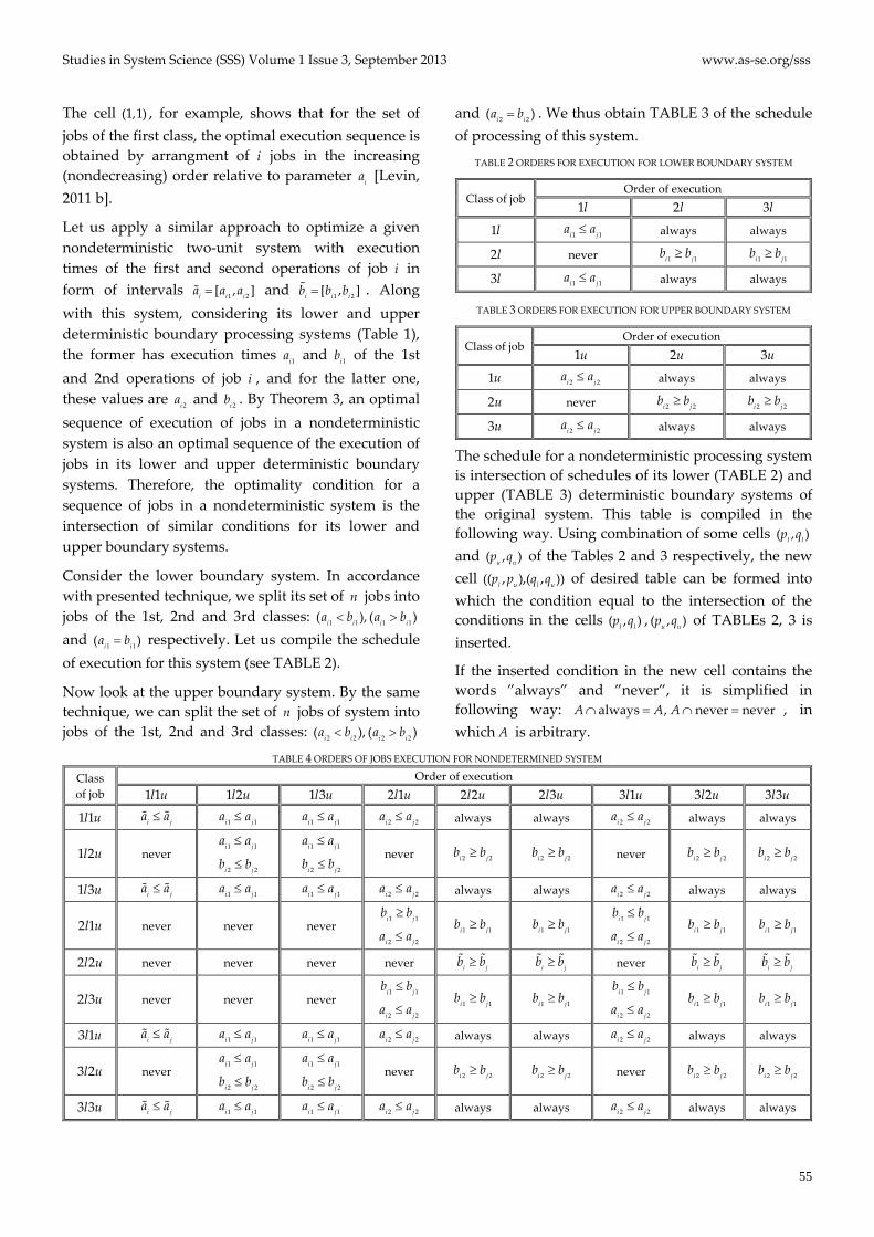
Consider the lower boundary system. In accordance with presented technique, we split its set of n jobs into jobs of the 1st, 2nd and 3rd classes: 1 1 1 1( ), ( )i i i ia b a b< > and 1 1( )i ia b= respectively. Let us compile the schedule of execution for this system (see TABLE 2).

Now look at the upper boundary system. By the same technique, we can split the set of n jobs of system into jobs of the 1st, 2nd and 3rd classes: 2 2 2 2( ), ( )i i i ia b a b< >

and 2 2( )i ia b= . We thus obtain TABLE 3 of the schedule of processing of this system.

TABLE 2 ORDERS FOR EXECUTION FOR LOWER BOUNDARY SYSTEM


1l 2l 3l

1l 1 1i ja a≤ always always

2l never 1 1i jb b≥ 1 1i jb b≥

3l 1 1i ja a≤ always always

TABLE 3 ORDERS FOR EXECUTION FOR UPPER BOUNDARY SYSTEM


1u 2u 3u

1u 2 2i ja a≤ always always

2u never 2 2i jb b≥ 2 2i jb b≥

3u 2 2i ja a≤ always always

The schedule for a nondeterministic processing system is intersection of schedules of its lower (TABLE 2) and upper (TABLE 3) deterministic boundary systems of the original system. This table is compiled in the following way. Using combination of some cells ( , )l lp q and ( , )u up q of the Tables 2 and 3 respectively, the new cell (( , ),( , ))l u l up p q q of desired table can be formed into which the condition equal to the intersection of the conditions in the cells ( , )l lp q , ( , )u up q of TABLEs 2, 3 is inserted.

If the inserted condition in the new cell contains the words ”always” and ”never”, it is simplified in following way: always , never neverA A A∩ = ∩ = , in which A is arbitrary.

TABLE 4 ORDERS OF JOBS EXECUTION FOR NONDETERMINED SYSTEM

Class of job

Order of execution 1 1l u 1 2l u 1 3l u 2 1l u 2 2l u 2 3l u 3 1l u 3 2l u 3 3l u

1 1l u i ja a≤ 1 1i ja a≤ 1 1i ja a≤ 2 2i ja a≤ always always 2 2i ja a≤ always always

1 2l u never 1 1i ja a≤

2 2i jb b≤ 1 1i ja a≤

2 2i jb b≤ never 2 2i jb b≥ 2 2i jb b≥ never 2 2i jb b≥ 2 2i jb b≥


2 1l u never never never 1 1i jb b≥

2 2i ja a≤ 1 1i jb b≥ 1 1i jb b≥ 1 1i jb b≤

2 2i ja a≤ 1 1i jb b≥ 1 1i jb b≥

2 2l u never never never never i jb b≥ i jb b≥ never i jb b≥ i jb b≥

2 3l u never never never 1 1i jb b≤

2 2i ja a≤ 1 1i jb b≥ 1 1i jb b≥ 1 1i jb b≤

2 2i ja a≤ 1 1i jb b≥ 1 1i jb b≥


3 2l u never 1 1i ja a≤

2 2i jb b≤ 1 1i ja a≤

2 2i jb b≤ never 2 2i jb b≥ 2 2i jb b≥ never 2 2i jb b≥ 2 2i jb b≥



56

The presented procedure is fulfilled for all possible combinations of cells in TABLEs 2 and 3. As a result, schedule for nondeterministic processing system (TABLE 4) is formed. In each cell (( , ),( , ))l u l up p q q of the TABLE 4, complex condition is presented under which the arbitrary jobs i and j (where job i belongs to the

lp -th class of the lower boundary system and to the

up -th class of the upper one and the job j belongs to the lq -th class of lower boundary system and to the

uq -th class of upper boundary system) are placed in an optimal sequence of execution of jobs in the order i j→ . These complex conditions in TABLE 4 are given in the form of inequalities for the boundaries of intervals determining the execution times of jobs and, when possible, in the form of inequalities for the indicated intervals.

For construction of non-exhaustive decision rules to determine all optimal sequences of executions of jobs in nondeterministic systems, we use TABLE 4. In contrast to determined systems, an optimal sequence of jobs execution in nondetermined systems may not exist. This is due to the fact that different intervals (execution times of jobs) may not be comparable and may not have minimal and maximal intervals [Levin, 2012]. The decision rules for each class of jobs forming the set of jobs which are performed in system are constructed separately.

Example

We will now construct the decision rule to find the optimal sequences of the execution of jobs corresponding to single class (1 ,1 )l u . At the TABLE 4 the condition in the cell ((1 ,1 ),(1 ,1 ))l u l u shows that jobs i in the sequences desired must follow in nondecressing order of interval parameter 1 2[ , ]i i ia a a= or, which is the same, in nondecreasing order of two parameters: 1ia and 2ia . What has been said implies the following rule: arrange all jobs i in nondecreasing order relative to the parameter 1ia and thus obtaining corresponding set 1M of ordered sequences of jobs; arrange all jobs i in nondecreasing order relative to parameter 2ia and obtain a similar set of sequences 2M ; take intersection of sets 1M and 2M which gives desired set of optimal sequences of jobs.

Optimization of the other systems with indeterminate parameters in which scheduling is absent can be carried out analogically to scheduling optimization in the systems [Levin, 2012, Mraz, Vatolin, Voshchinin]. We can use same mathematical apparatus of infinite-valued logic and logical determinants [Levin, 2011 b, 2012].

Conclusions

In this article, some theoretical facts in the field of jobs sequences in the systems has been illustrated, regarding some problems connected with uncertainty of time parameters of systems. It is shown that the problems can be reduce to complete determined case.

REFERENCES

Drummond, Mansford E. Evaluation and Measurement

Techniques for Digital Computer Systems. N.J.: Prentice-

Hall, 1973. 338 p.

Johnson, S.M. “Optimal Two-and-Three-Stage Production

Schedules with Set-up Times Included”. Naval Research

Logistic Quaterly 1 (1954): 61–68.

Levin, Vitaly I. (a) “System Optimization in Condition of

Interval Indeterminacy”. Paper presented at 18th

International Conference on Automatic Control

“Automatics-2011”, Lvov, Ukraine, 2011, pp. 51–58.

Levin, Vitaly I. (b) Scheduling Theory and Continuous Logic.

Saarbrücken: Lampert Academic Publishing, 2011.

Levin, Vitaly I. “Optimization in Terms of Interval

Uncertainty. The Determinization Method”. Automatic

Control and Computer Science 4 (2012): 157–163.

Mraz, F. “Calculating the Exact Bounds of Optimal Values in

LP with Interval Coefficients”. Annuals of Operation

Research 51 (1998): 51–62.

Muth, John F., Thompson, Gerald L. Industrial Scheduling.

N. J.: Prentice-Hall, 1963.

Vatolin, A.A. “Linear Programming with Interval Coeffici-

ents”. Computational Mathematics and Mathematical

Phy-sics 11 (1984): 1629–1637.

Voshchinin, A.P., Sotirov, G.R. Optimization in Condition of

Uncertainty. Moscow–Sofia: MEI Publishing House

(USSR), Technika (Bulgaria), 1989.