Download pdf - Shapiro - An Analysis of Variance Test for Normality (Complete Samples) 1965

8/3/2019 Shapiro - An Analysis of Variance Test for Normality (Complete Samples) 1965

http://slidepdf.com/reader/full/shapiro-an-analysis-of-variance-test-for-normality-complete-samples-1965 1/22

An Analysis of Variance Test for Normality (Complete Samples)

S. S. Shapiro; M. B. Wilk

Biometrika, Vol. 52, No. 3/4. (Dec., 1965), pp. 591-611.

Stable URL:

http://links.jstor.org/sici?sici=0006-3444%28196512%2952%3A3%2F4%3C591%3AAAOVTF%3E2.0.CO%3B2-B

Biometrika is currently published by Biometrika Trust.

Your use of the JSTOR archive indicates your acceptance of JSTOR's Terms and Conditions of Use, available athttp://www.jstor.org/about/terms.html. JSTOR's Terms and Conditions of Use provides, in part, that unless you have obtainedprior permission, you may not download an entire issue of a journal or multiple copies of articles, and you may use content inthe JSTOR archive only for your personal, non-commercial use.

Please contact the publisher regarding any further use of this work. Publisher contact information may be obtained athttp://www.jstor.org/journals/bio.html.

Each copy of any part of a JSTOR transmission must contain the same copyright notice that appears on the screen or printedpage of such transmission.

JSTOR is an independent not-for-profit organization dedicated to and preserving a digital archive of scholarly journals. Formore information regarding JSTOR, please contact [email protected].

http://www.jstor.orgMon May 21 11:16:44 2007


http://www.jstor.org/about/terms.html

http://www.jstor.org/journals/bio.html

http://www.jstor.org/journals/bio.html

http://www.jstor.org/about/terms.html




B i omet r i ka (1965), 52, 3 a n d 2 , p. 5 91

W i t h 5 t ex t - j gures

Printed in &eat Bri tain

An analysis of variance test fo r normality

(com plete samp1es)t

BYS. S. SHAPIRO AND M. B. WILK

General Electric Go. and Bell Telephone Laboratories, Inc.

The main intent of this paper is to introduce a new statistical procedure for testing a

complete sample for normality. The test statistic is obtained by dividing the square of an

appropriate linear combination of the sample order statistics by the usual symmetric

estimate of variance. This ratio is both scale and origin invariant and hence the statistic

is appropriate for a test of the composite hypothesis of normality.Testing for distributional assumptions in general and for normality in particular has been

a major area of continuing statistical research-both theoretically and practically. A

possible cause of such sustained interest is that many statistical procedures have been

derived based on particular distributional assumptions-especially that of normality.

Although in many cases the techniques are more robust than the assumptions underlying

them, still a knowledge that the underlying assumption is incorrect may temper the use

and application of the methods. Moreover, the study of a body of data with the stimulus

of a distributional test may encourage consideration of, for example, normalizing trans-

formations and the use of alternate methods such as distribution-free techniques, as well as

detection of gross peculiarities such as outliers or errors.

The test procedure developed in this paper is defined and some of it s analytical propertiesdescribed in $2. Operational information and tables useful in employing the tes t are detailed

in $ 3 (which may be read independently of the rest of the paper). Some examples are given

in $4. Section5 consists of an extract from an empirical sampling study of the comparison of

the effectiveness of various alternative tests. Discussion and concluding remarks are given

in $6.

2. THE W TEST FOR NORMALITY (COMPLETE SAMPLES)

2.1. Motivation and early work

This study was initiated, in pa rt, in an at tempt to summarize formally certain indications

of probability plots. In particular, could one condense departures from statistical linearity

of probability plots into one or a few 'degrees of freedom' in the manner of the application

of analysis of variance in regression analysis?

In a probability plot, one can consider the regression of the ordered observations on the

expected values of the order statistics from a standardized version of the hypothesized

distribution-the plot tending to be linear if the hypothesis is true. Hence a possible method

of testing the distributional assumptionis by means of an analysis of variance type procedure.

Using generalized least squares (the ordered variates are correlated) linear and higher-order

models can be fitted and an 3'-type ratio used to evaluate the adequacy of the linear fit.

t Pa rt of this research was supported by the Office of Naval Research while both authors were a t

Rutgers University.



This approach was investigated in preliminary work. While some promising results

were obtained, the procedure is subject to the serious shortcoming t ha t the selection of the

higher-order model is, practically speaking, arbitrary. However, research is continuing

along these lines.

Another analysis of variance viewpoint which has been investigated by the present

authors is to compare the squared slope of the probability plot regression line, which under

the normality hypothesis is an estimate of the population variance multiplied by a constant,

with the residual mean square about the regression line, which is another estimate of the

variance. This procedure can be used with incomplete samples and has been described

elsewhere (Shapiro & Wilk, 1965b).

As an alternative to the above, for complete samples, the squared slope may be com-

pared with the usual symmetric sample sum of squares about t he mean which is independent

of the ordering and easily computable. It is this last statistic that is discussed in the re-

mainder of this paper.

2.2. Derivation of the W statisticLet m' = (ml,m,, ...,m,) denote the vector of expected values of standard normal

order statistics, and let V = (vii) be the corresponding n x n covariance matrix. That is, if

x, 6 x, 6 . x, denotes an ordered random sample of size n from a normal distribution with

mean 0 and variance 1, then

E ( x ) ~=mi (i = 1,2, ...,n),

and cov (xi, xj) = vii (i,j = 1,2, ...,n) .

Let y' = (y,, ...,y,) denote a vector of ordered random observations. The objective is

to derive a test for the hypothesis that this is a sample from a normal distribution with

unknown mean p and unknown variance a,.

Clearly, if the {y,} are a normal sample then yi may be expressed as

y i = p + r x i ( i = 1,2,...,n).

It follows from th e generalized least-squares theorem (Aitken, 1938; Lloyd, 1952) th at t he

best linear unbiased estimates of p and a are those quantities th at minimize the quadratic

form (y -p l -am )' V-l (y -p l --a m), where 1' = (1,1, ...,1). These estimates are, respec-

tively,m' V-I ( ml'- lm') V-ly

'LI = 1'v-llm1v-lm- (11v-lm)2

1' V-l(l??a'-ml') V-lyand a = 1'8-I 1m'V-lm- (1'V-1m)2'

For symmetric distributions, 1'V-lm =0, and hence

A m' 7 - l ~= - y = , and 8 = -----n 1 m' V-lm'

Let

denote the usual symmetric unbiased estimate of (n- 1)a2.

The W test statist ic for normality is defined by



An an aly sis of variance test for no rm alit y

where

m' V-Ia' = (a,, ...,a,) =

(rn'V-1 V-lm)t

and

Thus, b is, up to the normalizing constant C, the best linear unbiased estimate of the slope

of a linear regression of the ordered observations, y,, on the expected values, mi, of the stand-

ard normal order statistics. The constant C is so defined th at the linear coefficients are

normalized.

It may be noted tha t if one is indeed sampling from a normal populatioii then the numer-

ator, b2,and denominator, S2,of W are both, up to a constant, estimating the same quantity,

namely a2.For non-normal populations, these quantities would not in general be estimating

the same thing. Heuristic considerations augmented by some fairly extensive empirical

sampling results (Shapiro & Wilk, 1964~)sing populations with a wide range of and

p2 values, suggest that the mean values of W for non-null distributions tends to shift

to the left of th at for the null case. Purther i t appears tha t the variance of the null dis-

tribution of W tends to be smaller than tha t of the non-null distribution. It is likely

that this is due to the positive correlation between the numerator and denominator for a

normal population being greater than th at for non-normal populations.

Note that the coefficients (a,) are just the normalized 'best linear unbiased' coefficients

tabulated in Sarhan & Greenberg (1956).

2.3. Some analytica2 properties of W

LEMMA. W is scale and origin invariant

Proof. This follows from the fact that for normal (more generally symmetric) distribu-tions,

COROLLARY. W has a distribution which depends only on the sanzple size n, for samples

from a normal distribution.

COROLLARYW is statistically independent of S2 and of 5, for samples from a normal.

distribution.

Proof. This follows from the fact that y and S2are sufficient for p and a2(Hogg & Craig,

1956).

COROLLARY = for any r.. E Wr Eb2r/ES2r,

LEMMA. The maximum value of W is 1. Proof. Assume?j= 0 since W is origin invariant by Lemma 1. Hence

Since

because X a: = a'a = 1, by definition, then W is bounded by 1. This maximum is in fact.I

achieved when yi = va,, for arbitrary 7.

LEMMA. The minimum value of TV is na!/(n - 1).



Pr0of.t (Due to C. L. Mallows.) Since W is scale and origin invariant, i t suffices to con-n

sider the maximization of 2; y! subject to the constraints Z y i = 0, Zaiy i = 1. Since thisi=l

is a convex region and Z y? is a convex function, the maximum of the latter must occur at

one of the ( n- 1) vertices of the region. These are

1 1 - (n- 1)9 9

( % ( a ,+ ...+a,-,)' n(al+ ...+a,-,) n(al+ .. +a, - ;Ja

It can now be checked numerically, for the values of the specific coefficients {a,), that the

n

maximum of 2; y: occurs at the first of these points and the corresponding minimum valuei= l

of W is as given in the Lemma.

LEMMA. Th e half an dfirst mom ents of W are given by

and

where R 2 = m l V - l m , and C 2=mlV-l V-lm.

Proof. Using Corollary 3 of Lemma 1,

E W* = EbIES and E W = E b 2 / E S 2 .

n - 1'/ ( and E S 2 = ( n - I ) @ .

From the general least squares theorem (see e.g. Kendall & Stuar t, vol. 11 (1961)),

and

since var (8)= a 2 / m 'V- lm = a 2 / R 2 ,and hence the results of the lemma follosv.

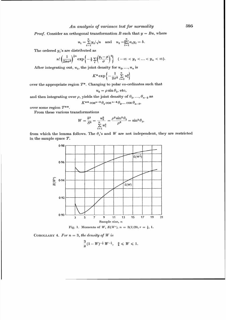
Values of these momen'ts are shown in Pig. 1 for sample sizes n = 3(1)20.

LEMMA. A joint distribution involving W i s defined b y

over a region T on w hich the Oi's and W are not ind epe nde nt, and where K is a constant.

1- Lemma 3 was conjectured intu itively and verified by certain numerical studies. Subsequently

the above proof was given by C. L. Mallows.

mailto:ES2=(n-I)@

mailto:ES2=(n-I)@



An an alys is of variance test for no rm ality

Proof.Consider an orthogonal transformation B such tha t y = Bu, where

12 12

u,= Cyi/@t and u2=lXaiyi= b.i=l i = l

The ordered y,'s are distributed as

After integrating out , u,, the joint density for u,, ...,u, is

over the appropriate region T*.Changing to polar co-ordinates such that

u2 = psinO,, etc,

and then integrating over p, yields the joint density of O,, ...,On-, as

K** cosn-3 0, cos n-4 02... cos On-3,over some region T**.

From these various transformations

, b2- - u? - p2sill20, = sin2O,,8 2 12

X .$ p2i= lfrom which the lemma follows. The Oi's and W are not independent, they are restricted

in the sample space T.

Sample size, 9%

Fig. 1. Moments of W, E(Wp) ,n = 3(1)20,s = +,1.

COROLLARY = 3, the density of W is. For n



Note that for n = 3, the it' statistic is equivalent (up to a constant multiplier) to the

statistic (rangelstandard deviation) advanced by David, Hartley & Pearson (1954) and

the result of the corollary is essentially given by Pearson & Stephens (1964).

It has not been possible, for general n, to integrate out of the 8,'s of Lemma 5 to obtain

an explicit form for the distribution of W. However, explicit results have also been given

for n = 4, Shapiro (1964).

2.4. Approxirnatio~zsssociated with the W test

The {a,) used in the W statistic are defined by

nai = C rnjvij/C ( j= 1,2,. n),

j=1

where rnj,vi j and C have been defined in $2.2. To determine the ai directly it appears necessary

to know both the vector of means m and the covariance matrix V. However, to date , the

elements of V are known only up to samples of size 20 (Sarhan & Greenberg, 1956). Variousapproximations are presented in the remainder of this section to enable the use of W for

samples larger than 20.

By definition, nz' V-I nz' 8-I

a = - -. -(nz'V-1 v-lnt)B - C

is such that a'a = 1. Let a* =m'V-1, then C2 = u*'a*. Suggested approximations are

= 2nzi (i = 2, 3, .. n - 1),

and

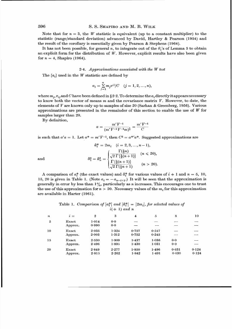
A comparisoil of a (the exact values) and ti: for various values of i $. 1 and n = 5, 10,

15, 20 is given in Table 1. (Note a4= - It will be seen tha t the approximation is

generally in error by less than 1% ,particularly as n increases.This encourages one to trust

the use of this approximation for n > 20. Necessary values of the mi for this approximation

are available in Harter (1961).

Table 1. Comparison of la$/ and \ti; = 12nz,l, for selected values of

i ( + 1) and n

Exact

Approx.

Exact

Approx.

Exact

Approx.

Exact

Approx.



597n an alys is of va riance test for nor ma lity

A comparison of a: and & for n = 6(1) 20 is given in Table 2. While the errors of this

approximation are quite small for n < 20, the approximation and true values appear to

cross over a t n = 19. Further comparisons with other approximations, discussed below,

suggested the changed formulation of 8: for n > 20 given above.

Table 2. Comparison of a: and & f

7% Exact Approximate " i ~ Exact Approximate

6sable but the

Sample size, 1%

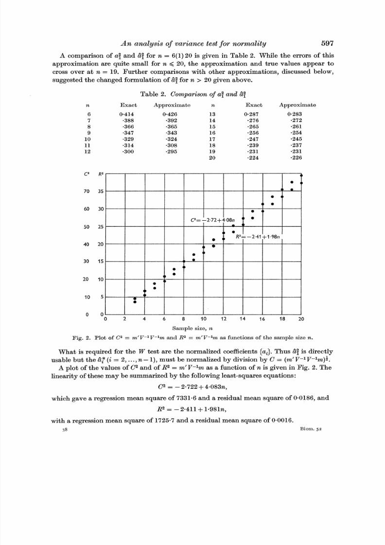
Fig. 2. Plot of C2 = m'V-lV-lm of the sample size n.nd R2 = m'V-lm as f~~nction s

What is required for the W test are the normalized coefficients {a,). Thus & f is directly

(i= 2, ...,n - 1), must be normalized by division by C = (m' V-1 V-lm ):.

A plot of the values of C 2and of R 2 = m' V- lm as a function of n is given in Fig. 2. The

linearity of these may be summarized by the following least-squares equations:

which gave a regression mean square of 7331.6 and a residual mean square of 0.0186, and

with a regression mean square of 1725.7 and a residual mean square of 0.0016.

Biom. j z8



These results encourage the use of the extrapolated equations to estimate C2 and R2

for higher values of n.

A comparison can now be made between values of C2 from the extrapolation equation12

and from using1

For the case n = 30, these give values of 119.77 and 120 .47 , respectively. This concordance

of the independent approximations increases faith in both.

Plackett (1958) has suggested approximations for the elements of the vector a and R2.

While his approximations are valid for a wide range of distributions and can be used with

censored samples, they are more complex, for the normal case, than those suggested above.

For the normal case his approximations are

where F ( m j ) = cumulative distribution evaluated a t mj,

f(naj)= density function evaluated a t mj,

and a"*1 =- a"*n s

Plackett's approximation to R2 is

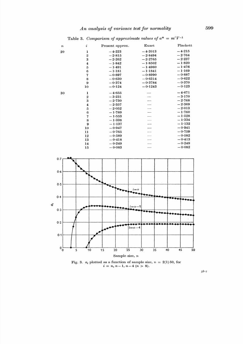
Plackett's a"," approximations and the present approximations are compared with the

exact values, for sample size 20 , in Table 3. I n addition a consistency comparison of the

two approximations is given for sample size 30 . Plackett's result for a, (n= 20) was the

only case where his approximation was closer to the true value than the simpler approxima-

tions suggested above. The differences in the two approximations for a, were negligible,

being less than 0 .5 %. Both methods give good approximations, being off no more than

three units in the second decimal place. The comparison of the two methods for n = 3 0

shows good agreement, most of the differences being in the third decimal place. The largest

discrepancy occurred for i = 2 ; the estimates differed by six units in the second decimal

place, an error of less than 2 %.

The two methods of approximating R2 were compared for n = 20 . Plackett's method

gave a value of 36.09, the method suggested above gave a value of 37.21 and the true

value was 37.26.

The good practical agreement of these two approximations encourages the belief tha t

there is little risk in reasonable extrapolations for n > 20. The values of constants, for

n > 20, given in $ 3 below, were estimated from the simple approximations and extrapola-

tions described above.

As a further internal check the values of a,, a,-, and a,-, were plotted as a function of

n for n = 3(1) 50 . The plots are shown in Fig. 3 which is seen to be quite smooth for each

of the three curves a t the value n = 20. Since values for n < 20 are 'exact' the smooth

transition lends credence to the approximations for n > 20 .



A n analysis o variance test for normality

Table 3 . Comparison of approximate values of a* = m'V-l

Present approx. Exact Placltett- 4.223 - 4.215

- 2.815 -2.764- 2.262 - 2.237- 1.842 - 1.820- 1.491 - 1.476- 1.181 - 1.169-0.897 - 0.887- 0.630 - 0.622- 0.374 - 0.370- 0.124 -0.123- 4.655 -4.671- 3.231 - 3.170- 2.730 - 2.768- 2.357 - 2.369

- 2.052-

2.013- 1.789 - 1.760- 1.553 - 1.528- 1.338 - 1.334- 1.137 - 1.132-0.947 - 0.941- 0.765 - 0.759-0.589 - 0.582- 0.418 - 0.413- 0.249 - 0.249- 0.083 - 0.082

Sample size, ra

Fig. 3. a, plotted as a function of sample size, ?z = 2(1) 50, for

i = n, n - 1, n - 4 (n > 8).



1.oo

0.95

0.90

0.85

W

0.80

0 75

0 70\ /

0 650 5 10 15 20 25 30 35 40 45 50

Sample size, n

Fig. 5. Selected empirical percentage points of W, n = 3(1 )50.



An ana lys is of var ia nce test fo r no rm al i ty

Table 4. Some theoretical mome nts (p,) and

$1

0.9130

.go19

a9021

0.9082

.9120

.9175

.9215

.9260

0.9295

a9338

.9369

.9399

.9422

0.9445

.9470

.9492

.9509

.9527

0.9549

.9558

.9570

.9579

.9584

0.9598

-9607

.9615

a9624

-9626

0.9636

.9642

a9650

-9654

.9658

0.9662

.9670

.9677

~9678

a9682

0.0084

a9691

~ 9 6 9 4

-9695

a9701

0.9703

~9710

.9709

.9712

.9714

Monte Carlo

$2

0.005698

e005166

.004491

0.003390

.002995

~002470

e002293

.001972

0.001717

.001483

.001316

.001168

.001023

0.000964

.000823

.000810

.000711

.000651

0.000594

.000568

.000504

.000504

.00045S

0.000421

.000404

~000382

.000369

~000344

0.000336

.000326

.000308

.000293

.000265

0.000264

.000253

.000235

.000239

-000229

0.000227

.000212

.000196

.000193

.000192

0.000184

.000170

.000179

.000165

.000154

moments (2,)

f i ,A%

3

Pz- 0.5930- .8944- .8176- 1.1790- 1.3229- 1.3841- 1.5987- 1.6655- 1.7494- 1.7744- 1.7581- 1.9025

- 1.8876- 1.7968- 1.9468

-2.1391- 2.1305- 2.2761- 2.2827- 2.3984- 2.1862- 2.3517-2.3448-2.4978-2.5903-2.6964- 2.6090- 2.7288- 2.7997-2.6900-3.0181- 3.0166- 2.8574- 2.7965- 3.1566- 3.0679-3.3283

-3.1719

- 3.0740-3.2885- 3.2646-3.0803-3.1645- 3.3742- 3.3353- 3.2972-3.2810-3.3240



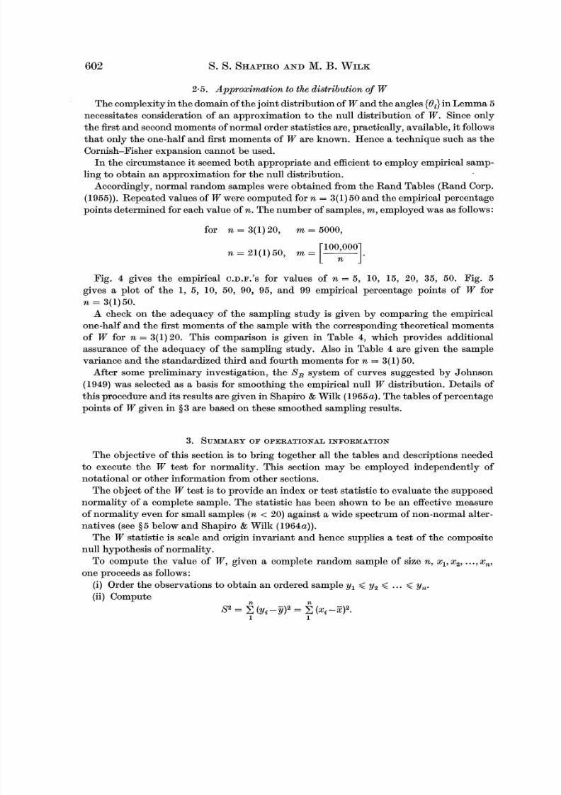
2.5. Approximation to the distribution of W

The complexity in the domain of the joint distribution of W and the angles (8,) in Lemma 5

necessitates consideration of an approximation to the null distribution of W. Since only

the first and second moments of normal order statistics are, practically, available, i t followsthat only the one-half and first moments of W are known. Hence a technique such as the

Cornish-Fisher expansion cannot be used.

I n the circumstance it seemed both appropriate and efficient to employ empirical samp-

ling to obtain an approximation for the null distribution.

Accordingly, normal random samples were obtained from the Rand Tables (Rand Corp.

(1955)). Repeated values of W were computed for n = 3(1)50 and the empirical percentage

points determined for each value of n. The number of samples, m, employed was as follows:

for n = 3(1)20, m = 5000,

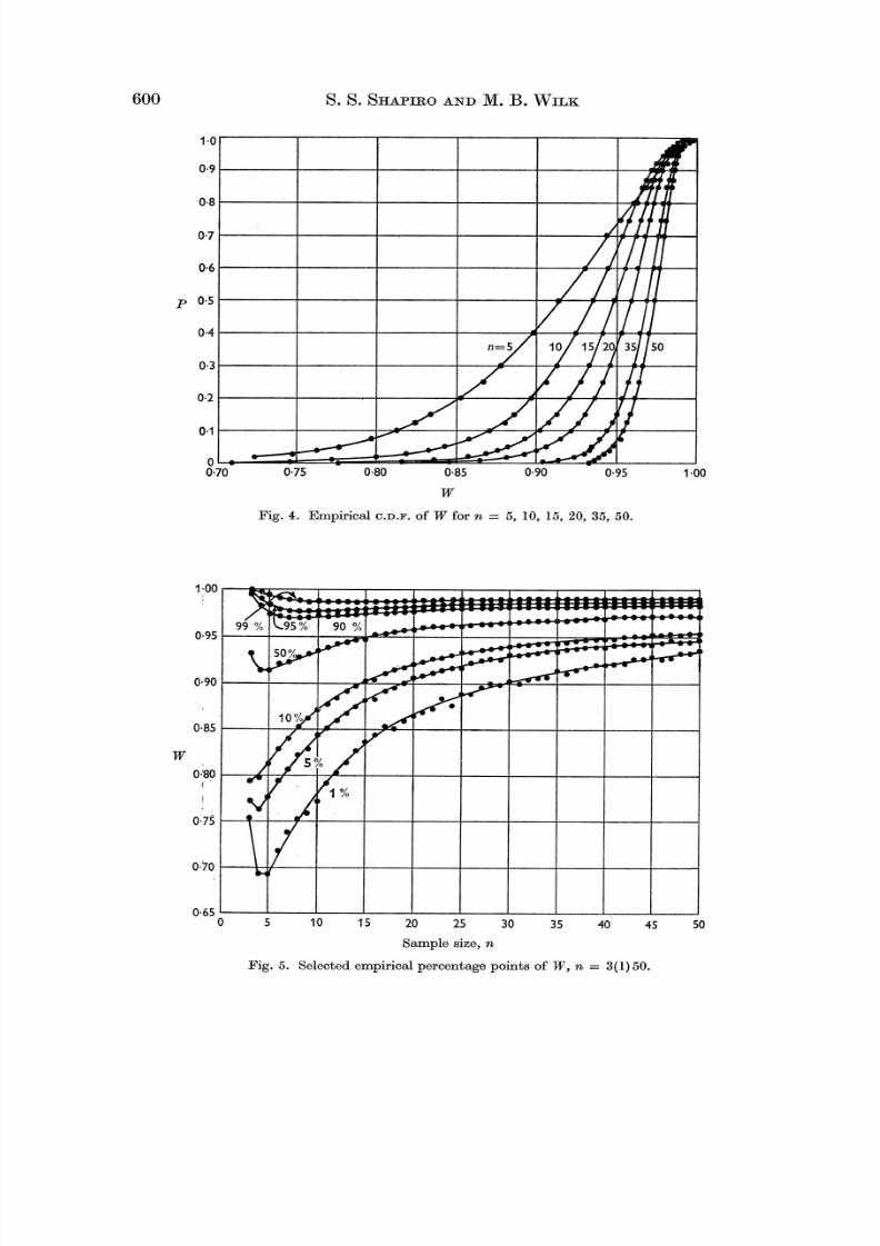
Fig. 4 gives the empirical G.D.F.'s for values of n = 5, 10, 15, 20, 35, 50. Fig. 5

gives a plot of the 1, 5 , 10, 50, 90, 95, and 99 empirical percentage points of W for

n = 3(1)50.

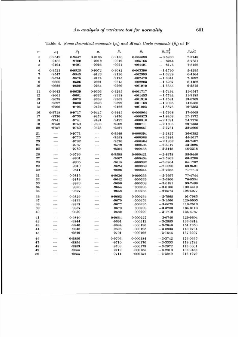
A check on the adequacy of the sampling study is given by comparing the empirical

one-half and the first moments of the sample with the corresponding theoretical moments

of W for n = 3(1)20. This comparison is given in Table 4, which provides additional

assurance of the adequacy of the sampling study. Also in Table 4 are given the sample

variance and the standardized third and fourth moments for n = 3(1)50.

After some preliminary investigation, the 8, system of curves suggested by Johnson

(1949) was selected as a basis for smoothing the empirical null W distribution. Details of

this procedure and its results are given in Shapiro & Wilk (1965~).he tables of percentage

points of W given in $3 are based on these smoothed sampling results.

The objective of this section is to bring together all the tables and descriptions needed

to execute the W test for normality. This section may be employed independently of

notational or other information fsom other sections.

The object of the W test is to provide a n index or test statistic to evaluate the supposed

normality of a complete sample. The statistic has been shown to be an effective measureof normality even for small samples (n < 20) against a wide spectrum of non-normal alter-

natives (see $ 5 below and Shapiro & Wilk (1964a)).

The W statistic is scale and origin invariant and hence supplies a tes t of the composite

null hypothesis of normality.

To compute the value of W, given a complete random sample of size n, x,, x2, ..,x,,

one proceeds as follows:

(i) Order the observations to obtain an ordered sample y, < y, < . . < y,,.

(ii) Computen 12

8 2 = I;(yi- g)2 = C (xi-q2.1 1



An ana lysis of variance test for nor ma lity

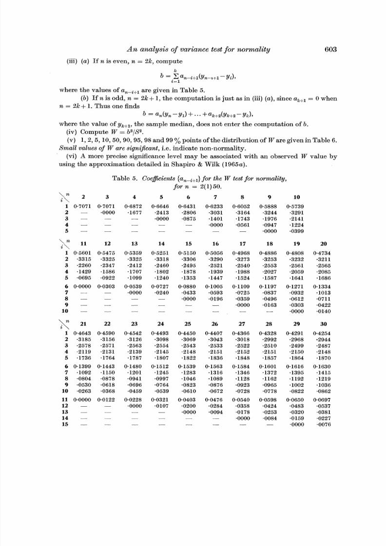
(iii) (a ) If n is even, n = 2E, compute

where the values of an-,+, are given in Table 5.

(b ) If n is odd, n = 2E+ 1, the computation is just as in (iii) (a),since a,+, = 0 when

?z = 2E+ 1. Thus one finds

b = an(yn-Y,) + ... +a,+2(Yk+2-~,)>

where the value of y,+,, the sample median, does not enter the computation of b.

(iv) Compute W = b2/S2.

(v) 1,2 ,5, 10,50,90,95,98 and 99 % points of the distribution of Ware given in Table 6.

Small values of W are significant, i.e. indicate non-normality.

(vi) A more precise significance level may be associated with an observed W value by

using the approximation detailed in Shapiro & Wilk (1965a).

Table 5. Coeficients {a,-,+,) for the W test for normality,

for n = 2(1)50.



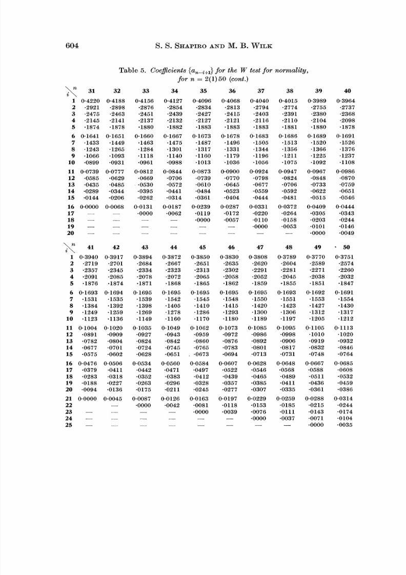
Table 5 . Co f i c i en t s {a,-i+,) for the W test for nor mal i ty ,

fo r n = 2(1)50 (cont.)



An an aly sis of variance test for no rm alit y

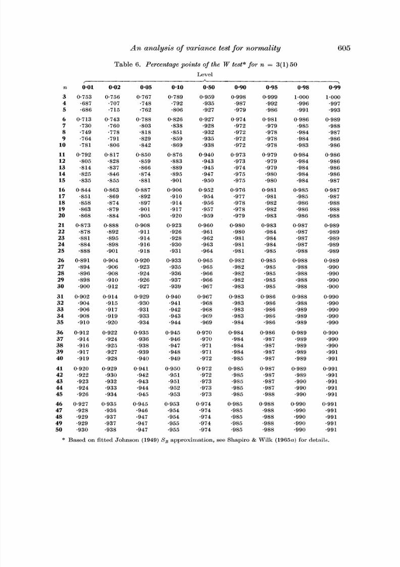
Table 6. Percentage points of the W test* for n = 3(1)50

Level

r A\

n 0.01 0.02 0-05 0.10 0.50 0.90 0.95 0.98 0.99

3 0.753 0.756 0.767 0.789 0.959 0.998 0.999 1.000 1.000

4 a687 a707 a748 a792 a935 .987 .992 .996 a997

5 .686 a715 .762 a806 .927 .979 ,986 .991 .993

6 0.713 0.743 0.788 0.826 0.927 0.974 0.981 0.986 0.989

7 .730 a760 .803 a838 a928 a972 a979 a985 ,988

8 .749 a778 .818 a851 a932 a972 a978 a984 .987

9 a764 .791 a829 a859 a935 .972 .978 a984 .986

10 a781 a806 a842 a869 a938 .972 .978 a983 a986

11 0.792 0.817 0.850 0.876 0.940 0.973 0.979 0.984 0.986

12 a805 a828 .859 a883 a943 a973 .979 .984 a986

13 a814 a837 ,866 a889 a945 a974 a979 .984 a986

14 .825 a846 a874 a895 .947 a975 ,980 a984 .986

15 .835 a855 .881 .90P a950 a975 ,980 .984 .987

16 0.844 0.863 0.887 0.906 0.952 0.976 0.981 0.985 0.987

17 a851 .869 a892 a910 a954 a977 a981 a985 a987

18 a858 a874 a897 a914 a956 a978 a982 a986 .988

19 .863 .879 .901 .917 a957 .978 -982 a986 a988

20 .868 a884 .905 a920 a959 .979 .983 a986 -988

21 0.873 0.888 0.908 0.923 0.960 0.980 0.983 0.987 0.989

22 .878 .892 a911 a926 a961 .980 ,984 .987 .989

23 .881 .895 .914 a928 ~ 9 6 2 a981 .984 .987 ~989

24 a884 a898 a916 a930 a963 a981 a984 a987 a989

25 a888 a901 .918 .931 .964 .981 .985 a988 .989

26 0.891 0.904 0.920 0.933 0.965 0.982 0.985 0.988 0.989

27 a894 a906 a923 .935 .965 a982 a985 a988 a990

28 a896 a908 a924 a936 .966 a982 .985 a988 a990

29 .898 a910 ,926 .937 .966 .982 ,985 a988 .990

30 a900 .912 a927 a939 a967 .983 a985 a988 a900

3 1 0.902 0.914 0.929 0.940 0.967 0.983 0.986 0.988 0.990

32 .904 a915 a930 .941 a968 a983 a986 a988 a990

33 a906 .917 a931 .942 a968 a983 a986 a989 a990

34 .908 a919 .933 a943 .969 a983 .986 a989 ,990

35 a910 .920 a934 a944 .969 a984 a986 a989 .990

36 0.912 0.922 0.935 0.945 0.970 0.984 0.986 0.989 0.990

37 a914 .924 .936 a946 a970 ,984 a987 a989 a990

38 a916 a925 a938 a947 a971 a984 .987 a989 ,990

39 .917 ,927 .939 .948 .97l a984 a987 a989 a991

40 a919 a928 a940 a949 a972 a985 a987 a989 a991

41 0.920 0.929 0.941 0.950 0.972 0.985 0.987 0.989 0.991

42 a922 a930 a942 a951 a972 .985 .987 a988 .991

43 a923 a932 a943 a951 a973 a986 .987 .990 .991

44 .924 .933 a944 .952 a973 a985 a987 a990 a991

45 a926 a934 .945 a953 .973 .985 a988 a990 a991

46 0.927 0.935 0.945 0.953 0.974 0.985 0.988 0.990 0.991

47 a928 a936 .946 a954 a974 .985 .988 a990 a991

48 a929 a937 .947 a954 ,974 a985 a988 ,990 ,991

49 a929 a937 a947 a955 a974 a985 a988 a990 a991

50 a930 .938 a947 a955 a974 a985 .988 a990 a991

* Based on fitted Johnson (1949) SB approximation, see Shapiro & Wilk (1965n) for detaild.



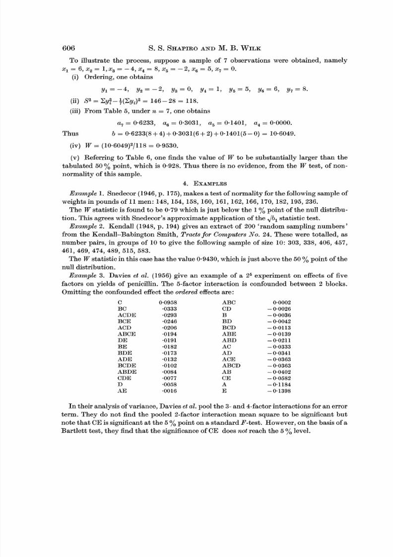
To illustrate th e process, suppose a sample of 7 observations were obtained, namely

x l = 6 , x 2 = 1 , x 3 =- 4 , x 4= 8 , x 5 = - 2 , x G = 5 , x 7 = 0.

(i) Ordering, one obtains

(iii) From Table 5, under ?z = 7, one obtains

Thus b = 0.6233(8+4)+0*3031(6+2)+0*1401(5-0) = 10.6049.

(iv) W = (10.6049)2/118= 0.9530.

(v) Referring to Table 6, one finds the value of W to be substantially larger than the

tabulated 50% point, which is 0.928. Thus there is no evidence, from the W test, of non-

normality of this sample.

Example 1. Snedecor (1946, p. 175), makes a test of normality for th e following sample of

weights in pounds of 11 men: 148, 154, 158, 160, 161, 162, 166, 170, 182, 195,236.

The W statistic is found to be 0.79 which is just below the 1% point of th e null distribu-

tion. This agrees with Snedecor's approximate application of the Jb , statistic test.

Example 2. Kendall (1948, p. 194) gives an extract of 200 'random sampling numbers'

from the Kendall-Babington Smith, Tracts for Computers No. 24. These were totalled , as

number pairs, in groups of 10 to give the following sample of size 10: 303, 338, 406, 457,

461, 469, 474, 489, 515, 583.

The W statistic in this case has th e value 0.9430, which is just above the 50% point of the

null distribution.

Example 3. Davies et al. (1956) give an example of a 25 experiment on effects of five

factors on yields of penicillin. The 5-factor interaction is confounded between 2 blocks.

Omitting the confounded effect the ordered effects are:

C AB C

B C C D

A C D E B

B C E B D

A C D B C D

A B C E A B E

D E A B D

B E AC

B D E A D

A D E A C E

B C D E A B C D

A B D E ,4B

C D E C E

D A

=SE E

I n their analysis of variance, Davies et al. pool the 3- and 4-factor interactions for an error

term. They do not find the pooled 2-factor interaction mean square to be significant bu t

note th at CE is significant at t he 5% point on a standard F-te st. However, on the basis of a

Bart lett tes t, they find th at t he significance of CE does not reach the 5% level.



607n ana lys is of variance test for nor ma lity

The overall statistical configuration of the 30 unconfounded effects may be evaluated

against a background of a null hypothesis tha t these are a sample of size 30 from a normal

population. Computing the W statistic for this hypothesis one finds a value of 0.8812,

which is substantially below the tabulated 1% point for the null distribution.

One may now ask whether the sample of size 25 remaining after removal of the 5 main

effects terms has a normal configuration. The corresponding value of W is 0.9326, which is

above the 10% point of the null distribution.

To investigate further whether the 2-factor interactions taken alone may have a non-

normal configuration due to one or more 2-factor interactions which are statistically

'too large', the W statistic may be computed for the ten 2-factor effects. This gives

which is well above the 50% point, for n = 10.

Similarly, the 15 combined 3 and 4-factor interactions may be examined from the same

point of view. The W value is 0.9088, which is just above the 10% value of the null distribu-

tion.

Thus this analysis, combined with an inspection of the ordered contrasts, would suggest

that the A, C and E main effects are real, while the remaining effects may be regarded as a

random normal sample. This analysis does not indicate any reason to suspect a real CE

effect based only on the statistical evidence.

The partitioning employed in this latter analysis is of course valid since the criteria

employed are independent of the observations per se .

I n the situation of this example, the sign of the contrasts is of course arbitrary and hence

their distributional configuration should be evaluated on the basis of the absolute values,

as in half-normal plotting (see Daniel, 1959). Thus, the above procedure had better be

carried out using a half-normal version of the W tes t if that were available.

To evaluate the W procedure relative to other tests for normality a n empirical sampling

investigation of comparative properties was conducted, using a range of populations and

sample sizes. The results of this study are given in Shapiro & Wilk (1964a), only a brief

extract is included in the present paper.

The null distribution used for the study of the W test was determined as described

above. For all other statistics, except the x 2goodness of fit, the null distribution employed

was determined empirically from 500 samples. For the x2 test, standard x 2 table values

were used. The power results for all procedures and alternate distributions were derived

from 200 samples.

Empirical sampling results were used to define null distribution percentage points for

a combination of convenience and extensiveness in the more exhaustive study of which the

results quoted here are an extract. More exact values have been published by various

authors for some of these null percentage points. Clearly one employing the Kolmogorov-

Smirnov procedure, for example, as a statistical method would be well advised to employ

the most accurate null distribution information available. However, the present power

results are intended only for indicative interest rather than as a definitive description of a

procedure, and uncertainties or errors of several percent do not materially influence the

comparative assessment.



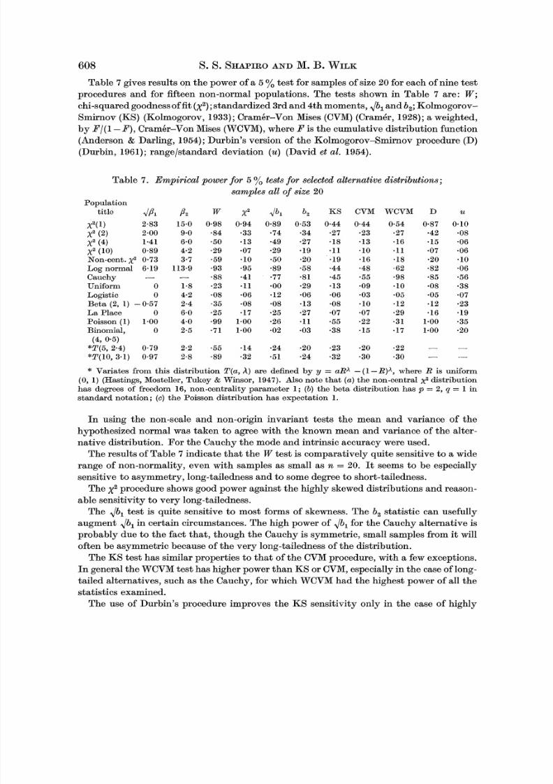
Table 7 gives results on the power of a 5% test for samples of size 20 for each of nine test

procedures and for fifteen non-normal populations. The tests shown in Table 7 are: W;

chi-squared goodnessof fit (x2 ); tandardized 3rd and 4th moments, Jbl and b,; Kolmogorov-

Smirnov (KS) (Kolmogorov, 1933);CramBr-Von Mises (CVM) (Cramdr, 1928) a weighted,

by Bl(1- P),CramBr-Von Mises (WCVM),where F is the cumulative distribution function

(Anderson & Darling, 1954); Durbin's version of the Kolmogorov-Smirnov procedure (D)

(Durbin, 196 1); rangelstandard deviation (u ) (David et al. 1954).

Table 7. Emp iricul power for 5% tests for selected alternative dist rib utio ~zs ;

samples all of size 20

Population

tit)le dP1 P2 W x2 <bl b2 KS CVM WCVM D u

x2(1) 2.83 15.0 0.98 0.94 0.89 0.53 0.44 0.44 0.54 0.87 0.10

~ " 2 ) 2.00 9.0 ~ 8 4 .33 .74 .34 .27 ~ 2 3 .27 .42 .08

x2 (4) 1.41 6.0 .50 +13 .49 .27 .I 8 .13 ~ 1 6 . I5 .06

x2 (10) 0.89 4.2 .29 .07 .29 .I9 . I1 . I0 ~ 1 1 ~ 0 7 .O6Non-cent.x20.73 3.7 .59 .10 .50 .20 .I9 .16 .I8 ~ 2 0 . l o

Lognormal 6.19 113.9 .93 ~ 9 5 .89 .58 .44 .48 .62 .82 so6

Cauchy - - .88 .41 .77 .81 .45 .55 .98 .85 .56

Uniform 0 1.8 ~ 2 3 .11 .00 .29 .13 .09 . I0 .08 ~ 3 8

Logistic 0 4.2 .08 .06 .12 ~ 0 6 .06 .03 .03 .05 .07

B e t a ( 2 , I ) - 0 . 5 7 2.4 .3 5 .08 .08 ~ 1 3 ~ 0 8 .10 .I2 .I2 a23

La Place 0 6.0 .25 .17 .25 .27 .07 .07 .29 .16 .19

Poisson (1) 1.00 4.0 ~ 9 9 1.00 .26 .I 1 ~ 5 5 .22 .31 1.00 .35

Binomial, 0 2.5 .71 1.00 .02 .03 ~ 3 8 .15 .I7 1.00 .20

(4, 0.5) "T(5,2.4) 0.79 2.2 ~ 5 5 ~ 1 4 .24 .20 .23 ~ 2 0 .22 - -;FT(lO, .1) 0.97 2.8 ~ 8 9 .32 ~ 5 1 .24 ~ 3 2 .30 .30 - -* Variates from this distribution T(a, A) are defined by y = aRh - (1 R)h, where R is uniform

(0, 1) (Hastings, Mosteller, Tukey & Winsor, 1947). Also note tha t (a) the non-central x 2 distribution

has degrees of freedom 16, non-centrality parameter 1 ; (b ) the beta distribution has p = 2, q = 1 in

standard notation; (c ) the Poisson distribution has expectation 1.

In using the non-scale and non-origin invariant tests the mean and variance of the

hypothesized normal was taken to agree with the known mean and variance of the alter-

native distribution. For the Cauchy the mode and intrinsic accuracy were used.

The results of Table 7 indicate th at the W test is comparatively quite sensitive to a wide

range of non-normality, even with samples as small as n = 20. It seems to be especially

sensitive to asymmetry, long-tailedness and to some degree to short-tailedness.

The x2procedure shows good power against the highly skewed distributions and reason-

able sensitivity to very long-tailedness.The db , test is quite sensitive to most forms of skewness. The b, statistic can usefully

augment db , in certain circumstances. The high power of Jb, for the Cauchy alternative is

probably due to the fact tha t, though the Cauchy is symmetric, small samples from it will

often be asymmetric because of the very long-tailedness of the distribution.

The KS test has similar properties to that of the CVM procedure, with a few exceptions.

I n general the WCVM tes t has higher power than KS or CVM, especially in the case of long-

tailed alternatives, such as the Cauchy, for which WCVM ha,d the highest power of all the

statistics examined.

The use of Durbin's procedure improves the KS sensitivity only in the case of highly



609n ana lys is of variance test for nor ma lity

skewed and discrete alternatives. Against the Cauchy, the D test responds, like db,,

to the asymmetry of small samples.

The u test gives good results against the uniform alternative and this is representative of

its properties for short-tailed symmetric alternatives.

The x2test has the disadvantages that the number and character of class intervals used

is arbitrary, th at all information concerning sign and trend of discrepancies is ignored and

th at , for small samples, the number of cells must be very small. These factors might explain

some of the lapses of power for x2 indicated in Table 7. Note that for almost all cases the

power of W is higher than th at of x2.

As expected, the db, test is in general insensitive in the case of symmetric alternatives

as illustrated by the uniform distribution. Note that for all cases, except the logistic,

,/b, power is dominated by that of the W test.

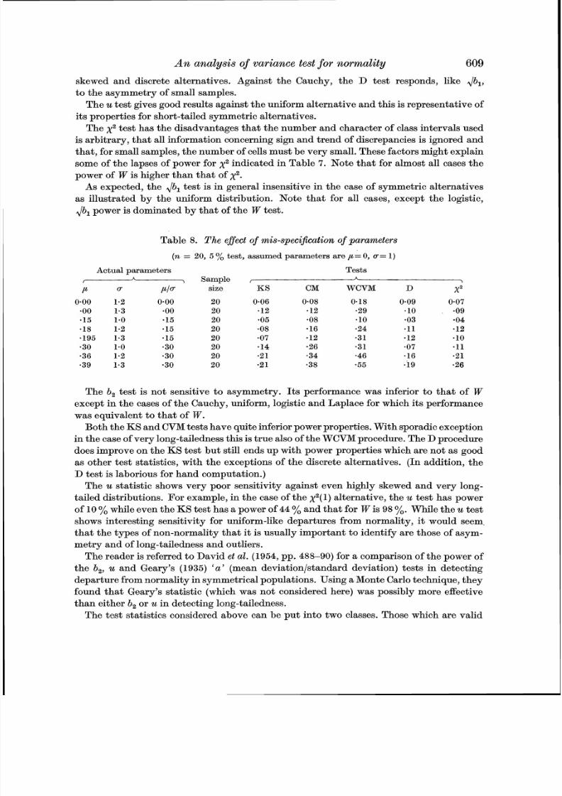
Table 8. The eflect of mis-specicaton of parameters

(1% = 20, 5 % test, assumed parameters are p= 0, a = 1)

Actual parameters Tests

,-A , Sample r A >

P 0- PI C size KS CM WCVM D x 2

The b, test is not sensitive to asymmetry. I ts performance was inferior to that of W

except in the cases of the Cauchy, uniform, logistic and Laplace for which its performance

was equivalent to th at of W.

Both the KS and CVM tests have quite inferior power properties. With sporadic exception

in the case of very long-tailedness this is true also of the WCVM procedure. The D procedure

does improve on the KS test but still ends up with power properties which are not as good

as other test statistics, with the exceptions of the discrete alternatives. (I n addition, the

D test is laborious for hand computation.)

The u statistic shows very poor sensitivity against even highly skewed and very long-

tailed distributions. For example, in the case of the x2(1) lternative, the u test has power

of 10% while even the KS test has a power of 44 % and that for W is 98 %. While the u testshows interesting sensitivity for uniform-like departures from normality, it would seem

th at the types of non-normality that it is usually important to identify are those of asym-

metry and of long-tailedness and outliers.

The reader is referred to David et ul. (1954, pp. 488-90) for a comparison of the power of

the b,, u and Geary's (1935) 'a ' (mean deviationlstandard deviation) tests in detecting

departure from normality in symmetrical populations. Using a Monte Carlo technique, they

found that Geary's statistic (which was not considered here) was possibly more effective

than either b, or u in detecting long-tailedness.

The test statistics considered above can be put into two classes. Those which are valid



GPO S. S. SHAPIROND M. B. WILK

for composite hypotheses and those which are valid for simple hypotheses. For the simple

hypotheses procedures, such as x2,KS, CVM, WCVM and D, the parameters of the null

distribution must be pre-specified. A study was made of the effect of small errors of specifica-

tion on the test performance. Some of the results of this study are given in Table 8. The

apparent power in the cases of mis-specification is comparable to that attained for theseprocedures against non-normal alternatives. For example, for p /a= 0.3, WCVM has

apparent power of between 0-31 and 0.55 while its power against x2(2) is only 0.27.

6. DISCUSSIONND CONCLUDING REMARKS

6.1. Evaluation of test

As a test for the normality of complete samples, the W statistic has several good features-

namely, that it may be used as a test of the composite hypothesis, that is very simple to

compute once the table of linear coefficients is available and th at the test is quite sensitive

against a wide range of alternatives even for small samples (n < 20). The statistic is re-

sponsive to the nature of the overall configuration of the sample as compared with the con-

figuration of expected values of normal order statistics.

A drawback of the W test is th at for large sample sizes i t may prove awkward to tabulate

or approximate the necessary values of the multipliers in the numerator of the statistic.

Also, it may be difficult for large sample sizes to determine percentage points of its dis-

tribution.

The W test had its inception in the framework of probability plotting. The formal use

of the (one-dimensional) test statistic as a methodological tool in evaluating the normality

of a sample is visualized by the authors as a supplement to normal probability plotting and

not as a substitute for it.

6.2. Extensions

It has been remarked earlier in the paper tha t a modification of the present W statisticmay be defined so as to be usable with incomplete samples. Work on this modified W*statistic will be reported elsewhere (Shapiro & Wilk, 19653).

The general viewpoint which underlies the construction of the W and W* tests for

normality can be applied to derive tests for other distributional assumptions, e.g. that a

sample is uniform or exponential. Research on the construction of such statistics, including

necessary tables of constants and percentage points of null distributions, and on their

statistical value against various alternative distributions is in process (Shapiro & Wilk,

19643). These statistics may be constructed so as to be scale and origin invariant and thus

can be used for tests of composite hypothesis.

It may be noted th at many of the results of $2.3 apply to any symmetric distribution.

The W statistic for normality is sensitive to outliers, either one-sided or two-sided.

Hence it may be employed as part of an inferential procedure in the analysis of experimental

data as suggested in Example 3 of $4.

The authors are indebted to Mrs M. H. Becker and Mis H. Chen for their assistance in

various phases of the computational aspects of the paper. Thanks are due to the editor

and referees for various editorial and other suggestions.



An a~ za lys is f variance test for norm ality 611

AITKEN,A. C. (1935). On least squares and linear combination of observations. Proc. Roy. Soc. Edin.

55, 42-8.

ANDERSON,. It7.& DARLING,D. A. (1954). A test for goodness of fit. J. Amer. Statist. Ass. 49 ,

765-9.

CRAMER,H. (1928). On the composition of elementary errors. Slcand. Aktuar. 11, 141-80.

DANIEL,C. (1959). Use of half-normal plots in interpreting factorial two level experiments. Techno-

metrics, 1, 311-42.

DAVID,H. A., HARTLEY, . 0. & PEARSON,. S. (1954). The distribution of the ratio, in a single

normal sample, of range to standard deviation. Biometrika, 41, 482-3.

DAVIES,0. L. (ed). (1956). Design and Analysis of Industrial Experiments. London: Oliver and Boyd.

DURBIN,J. (1961). Some methods of constructing exact tests. Biometrika, 48, 41-55.

GEARY,R. C. (1935). The ratio of the mean deviation to the s tandard deviation as a test of normality .

Biometrika, 27 , 310-32.

HARTER,H. L. (1961). Expected values of normal order statistics. Biometrika, 48 , 151-65.

HASTINGS,C., MOSTELLER,., TUKEY,J. & WINSOR,C. (1947). Low moments for small samples:

a comparative study of order statistics. Ann. Math. Statist. 18. 413-26.

HOGG, V. & CRAIG,"A.. (1956). S~lfficient tatistics in elementary distribution theory. Sankyd, 17 ,209-16.

JOHNSON,. L. (1949). Systems of frequency curves generated by methods of translation. Biometrika,

36, 149-76.

I<E~'u.~LL,. G. (1948). The Advanced Theory of Statistics, 1. London: C. Griffin and Co.

KENDALL, A. (1961).The Advanced Theory of Statistics, 2. London: C. Griffin and Co .. G. & STUART,

KOLMOGOROV, G. Ist. Att.-. N. (1933). Sulla determinazione empirica di une legge di distribuzione.

uari, 83-91.

LLOYD,E. H. (1952). Least squares estimation of location and scale parameters using order statistics.

Biometrika, 39 , 88-95.

PEARSON,. S. & STEPHENS,M. A. (1964). The ratio of range to standard deviation in the same

normal sample. Biometrika, 51, 484-7.

PLACKETT,. L. (1958). Linear estimation from censored data. An n. Math. Statist. 29 , 131-42.

RANDCORPORATION1955). A 1Willion Random Digits with 100,000 Normal Deviates.

SARHAN,A. E. & GREENBERG,. G. (1956). Estimation of location and scale parameters by order

statistics from singly and double censored samples. Pa rt I. An n. Math. Statist. 27, 427-51.

SHAPIRO,S. S. (1964). An analysis of variance test for normality (complete samples). Unpublished

Ph.D. Thesis, Rutgers-The State University.

SHAPIRO,. S. & WILK, M. B. (1964a). A comparative study of various tests for normality. Unpub-

lished manuscript . Invi ted paper, Amer. St at . Assoc, Annual Meeting, Chicago, Illinois, December

1964.

SHAPIRO,. S. & WILK, M. B. (1964b). Tests for the exponential and uniform distributions. (Unpub-

lished manuscript.)

SHAPIRO,. S. & WILK, M. B. (1965a). Testing the normality of several samples. (Unpublished

manuscript).

SHAPIRO,. S. & WILK,M. B. (1965b). An analysis of variance tes t for normality (incomplete samples).

(Unpublished manuscript.)

SNEDECOR, Ames: Iowa Sta te College Press.. W. (1946). Statistical Methods, 4th edition.