Download pdf - Single machine group scheduling with resource dependent setup and processing times

European Journal of Operational Research 162 (2005) 112–121

www.elsevier.com/locate/dsw

Single machine group scheduling with resourcedependent setup and processing times

Adam Janiak a, Mikhail Y. Kovalyov b, Marie-Claude Portmann c,*

a Institute of Engineering Cybernetics, Technical University of Wroclaw, Wroclaw 50372, Polandb Belarus State University, and United Institute of Informatics Problems, National Academy of Sciences of Belarus,

Minsk 220012, Belarusc MACSI team of INRIA-Lorraine and LORIA-INPL, Ecole des Mines de Nancy, Parc de Saurupt, Nancy Cedex 54042, France

Received 1 November 2001; accepted 1 November 2002

Available online 24 March 2004

Abstract

A single machine scheduling problem is studied. There is a partition of the set of n jobs into g groups on the basis of

group technology. Jobs of the same group are processed contiguously. A sequence independent setup time precedes the

processing of each group. Two external renewable resources can be used to linearly compress setup and job processing

times. The setup times are jointly compressible by one resource, the job processing times are jointly compressible by

another resource and the level of the resource is the same for all setups and all jobs. Polynomial time algorithms are

presented to find an optimal job sequence and resource values such that the total weighted resource consumption is

minimum, subject to meeting job deadlines. The algorithms are based on solving linear programming problems with

two variables by geometric techniques.

� 2004 Elsevier B.V. All rights reserved.

Keywords: Scheduling; Single machine; Group technology; Resource allocation; Linear programming

1. Motivation and literature review

We study a single machine scheduling problem with resource dependent setup and processing times

under group technology (GT) constraints.

GT is an approach to manufacturing and engineering management that seeks to achieve the efficiency ofhigh-volume production by exploiting similarities of different products and activities in their production/

execution. With respect to part manufacturing, the main idea of GT is to identify similar parts and classify

them into groups to take advantage of their similarities. After the parts are classified into groups, cells of

machines are configured and are dedicated to the production of specific groups of parts.

* Corresponding author.

E-mail addresses: [email protected], [email protected] (M.-C. Portmann).

0377-2217/$ - see front matter � 2004 Elsevier B.V. All rights reserved.

doi:10.1016/j.ejor.2002.11.004

mail to: [email protected],

A. Janiak et al. / European Journal of Operational Research 162 (2005) 112–121 113

In many applications, a major setup of the machine is needed for switching between the groups and aminor setup is needed for its switching between the jobs of the same group. When setup times are sequence

independent, the time requirement for a minor setup can be included in the processing time of the corre-

sponding job.

Studies of GT were originated by Mitrofanov [25] and Opitz [26]. Numerous manufacturing companies

have taken advantage of GT to improve productivity and competitiveness, see, for example, Ham et al. [14],

Wemmerlv and Hyer [35], Tatikonda and Wemmerlv [33], Hadjinicola and Ravi Kumar [13], and Gun-

asekaran et al. [12].

The first publications on scheduling in group technology environments are due to Petrov [27], andYoshida et al. [34]. Results on group scheduling problems are reviewed by Potts and Van Wassenhove [29]

and Liaee and Emmons [23]. Results not included in these reviews can be found in papers of Kovalyov and

Tuzikov [21], Janiak and Kovalyov [17], Janiak et al. [19], Liu and Yu [24].

Note that GT approach does not allow group splittings. In a more general batching approach, each

group can be partitioned into two or more batches processed separately, see Potts and Kovalyov

[28].

There are publications on scheduling problems without group technology constraints but with resource

dependent job processing times or release dates. Among them are papers by Janiak [15,16], Cheng andJaniak [6], Janiak and Portmann [20], Chen et al. [9], Janiak and Kovalyov [18], Li et al. [22], Cheng et al.

[5], Cheng et al. [10], Biskup and Jahnke [2]. Some models of this type are discussed in the monograph of

Blazewicz et al. [3].

It is natural to study the situations where group scheduling and resource allocation decisions are

combined.

A single machine batch scheduling problem with resource dependent parameters has been studied by

Cheng and Kovalyov [7] and Cheng et al. [8]. In this problem, there is a single group that can be partitioned

into batches and jobs of the same batch complete together when the latest job of this batch has finished itsprocessing. The processing of each batch is preceded by a common setup time. The former paper contains

complexity results, dynamic programming algorithms and approximation for the case when only the job

processing times are resource dependent. The latter paper assumes that the setup time is also resource

dependent and presents polynomial time algorithms for this case. To the best of our knowledge, there are

no other results available in the literature for group or batch scheduling problems with resource dependent

setup and/or processing times.

2. Problem formulation

We study the following problem.

There are n independent, non-preemptive and simultaneously available jobs to be scheduled for pro-

cessing on a single machine. A partition of the set of jobs into g groups is given. Jobs of the same group are

processed contiguously and cannot be split into subgroups processed separately. Each group Gf includes qfjobs,

Pgf¼1 qf ¼ n. A sequence independent machine setup time Sf precedes the processing of the first job of

group Gf , f ¼ 1; . . . ; g. Each job Jj has a processing time pj and a deadline dj, j ¼ 1; . . . ; n.The setup times are variables depending on an equal amount x of a renewable continuously divisible or

discrete resource used for their performing: sf ¼ af � bf x, where af is the value of sf for x ¼ 0 and bf is thevalue of the setup time reduction per unit of the resource, f ¼ 1; . . . ; g. It is assumed that x 2 ½0; xmax� andaf � bf xmax > 0, f ¼ 1; . . . ; g.

Similarly, the job processing times depend on an amount y of the same or another renewable resource:

pj ¼ rj � tjy; y 2 ½0; ymax�, rj � tjymax > 0, j ¼ 1; . . . ; n. It is assumed that both resources are either contin-

uous or discrete.

114 A. Janiak et al. / European Journal of Operational Research 162 (2005) 112–121

If the same resource is used to compress setups and processing times, then there is an additional con-straint xþ y6 emax. Assume that emax P maxfxmax; ymaxg. If xmax > emax or ymax > emax, then we can set

xmax ¼ emax or ymax ¼ emax, respectively, because inequalities xþ y6 emax and x; yP 0 imply x; y6 emax.

Assume without loss of generality that the resources are the same. The case of different resources can be

modeled by setting emax ¼ xmax þ ymax.

A solution specifies the values x and y of the resource and the job schedule. Given a solution, job

completion times Cj, j ¼ 1; . . . ; n, can be calculated. The objective is to find a solution such that the

deadlines are satisfied, i.e., Cj 6 dj for all j, and the total weighted resource consumption vxþ wy is min-

imized. All numerical data are assumed to be positive integers. Values v and w are assumed to be relativelyprime without loss of generality. Variables x and y are real numbers if the resource is continuously divisible

and they are integer numbers if the resource is discrete.

Observe that there exists an optimal schedule where the machine has no idle time until it finishes pro-

cessing of the latest job. Therefore, we consider such schedules only and assume that any schedule is

represented by the sequence of jobs within each group and the sequence of groups.

Adapting the three-field notation ajbjc of Graham et al. [11], we denote the above problem as

1ðGTÞjsf ¼ af � bf x, pj ¼ rj � tjy, h, Cj 6 djjvxþ wy, where h 2 fcntn; dscr; �g and � represents empty

symbol. If h ¼ cntn, then the resource is continuously divisible. If h ¼ dscr, then the resource is discrete. Ifh ¼ �, then the resource is either continuously divisible or discrete.

The rest of the paper is organized as follows. In Section 3, we study the special case called FIX, in which

the sequence of groups is fixed and y 2 ½Y1; Y2�, where 06 Y1 < Y2 6 ymax and Y1; Y2 are given rational

numbers. We present Oðn log nÞ and Oðn log2 maxfn;maxj ftjg; v;w; xmax; Y2gÞ time algorithms to solve

problem FIX if the resource is continuously divisible and discrete, respectively. In the following section, we

show that the original problem can be reduced in Oðn2 þ gnminfg; log ngÞ time to OðgnÞ problems FIX.

Hence, the original problem can be solved in Oðgn2 log nÞ and Oðgn2 log2 maxfn;maxj ftjg; v;w; xmax; ymaxgÞtime if the resource is continuously divisible and discrete, respectively. The cases when all processing timesare fixed or all setup times are fixed are studied in Section 5. Algorithms faster than the generic ones are

presented for these cases. The paper concludes with some remarks and suggestions for future research.

3. Problem FIX with a fixed group sequence

We begin our analysis of the problem 1ðGTÞjsf ¼ af � bf x; pj ¼ rj � tjy, Cj 6 djjvxþ wy with noting that

there exists an optimal schedule, if any such schedule exists, in which jobs of the same group are sequencedin the earliest deadline (ED) order, see Potts and Van Wassenhove [29].

Let G1; . . . ;Gg be the fixed group sequence. Consider solutions, in which the groups are sequenced

G1; . . . ;Gg, the jobs of each group are sequenced in the ED order and x 2 ½0; xmax�, y 2 ½Y1; Y2�, xþ y6 emax.

We show how to find values x0 and y0 such that Cj 6 dj for all jobs, and vxþ wy is minimized.

Denote by ðf ; jÞ the job sequenced as the jth in group Gf . A solution is feasible with respect, to the

deadlines if and only if

Xf�1

h¼1

sh

þXqhi¼1

pðh;iÞ

!þ sf þ

Xji¼1

pðf ;iÞ 6 dðf ;jÞ; j ¼ 1; . . . ; gf ; f ¼ 1; . . . ; g: ð1Þ

Since setup and processing times are resource dependent, rewrite (1) as the set of linear inequalities with

two variables x and y. Calculate

Rjf ¼

Xji¼1

rðf ;iÞ; T jf ¼

Xji¼1

tðf ;iÞ; Af ¼Xfh¼1

ah; Bf ¼Xfh¼1

bh; f ¼ 1; . . . ; g; j ¼ 1; . . . ; qf :


These calculations can be done in OðnÞ time becausePg

f¼1 qf ¼ n.Denote Rf ¼

Pfh¼1 R

qhh and Tf ¼

Pfh¼1 T

qhh . Then (1) together with the other restrictions on x and y can be

written as

ðAf þ Rf�1 þ Rjf Þ � Bf x� ðTf�1 þ T j

f Þy6 dð f ;jÞ;

f ¼ 1; . . . ; g; j ¼ 1; . . . ; qf ; 06 x6 xmax; 06 y6 ymax; xþ y6 emax: ð2Þ

3.1. Continuously divisible resource

Assume that x and y are real numbers. Observe that if xmax þ Y2 6 emax and the point ðx; yÞ ¼ ðxmax; Y2Þdoes not satisfy (2) for some f and j or if xmax þ Y2 > emax and no point ðemax � Y2; Y2Þ and ðxmax; emax � xmaxÞsatisfies (2), then there is no feasible solution to problem FIX. Furthermore, if the point ð0; Y1Þ satisfies (2),then x0 ¼ 0 and y0 ¼ Y1 minimize vxþ wy and determine a solution to problem FIX. Assume that the

feasibility of the above mentioned points has been checked. It can be done in OðnÞ time.

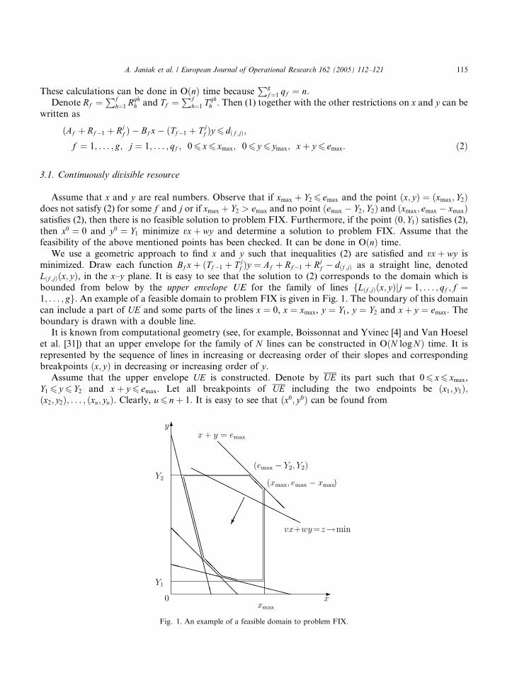
We use a geometric approach to find x and y such that inequalities (2) are satisfied and vxþ wy is

minimized. Draw each function Bf xþ ðTf�1 þ T jf Þy ¼ Af þ Rf�1 þ Rj

f � dðf ;jÞ as a straight line, denoted

Lðf ;jÞðx; yÞ, in the x–y plane. It is easy to see that the solution to (2) corresponds to the domain which is

bounded from below by the upper envelope UE for the family of lines fLðf ;jÞðx; yÞjj ¼ 1; . . . ; qf ; f ¼1; . . . ; gg. An example of a feasible domain to problem FIX is given in Fig. 1. The boundary of this domain

can include a part of UE and some parts of the lines x ¼ 0, x ¼ xmax, y ¼ Y1, y ¼ Y2 and xþ y ¼ emax. The

boundary is drawn with a double line.

It is known from computational geometry (see, for example, Boissonnat and Yvinec [4] and Van Hoesel

et al. [31]) that an upper envelope for the family of N lines can be constructed in OðN logNÞ time. It is

represented by the sequence of lines in increasing or decreasing order of their slopes and corresponding

breakpoints ðx; yÞ in decreasing or increasing order of y.Assume that the upper envelope UE is constructed. Denote by UE its part such that 06 x6 xmax,

Y1 6 y6 Y2 and xþ y6 emax. Let all breakpoints of UE including the two endpoints be ðx1; y1Þ;ðx2; y2Þ; . . . ; ðxu; yuÞ. Clearly, u6 nþ 1. It is easy to see that ðx0; y0Þ can be found from

Fig. 1. An example of a feasible domain to problem FIX.


vx0 þ wy0 ¼ minfvxþ wyjðx; yÞ 2 fðx1; y1Þ; . . . ; ðxu; yuÞgg:
Thus, if group sequence is fixed and y 2 ½Y1; Y2�, then the problem 1ðGTÞjsf ¼ af � bf x, pj ¼ rj � tjy,
cntn, Cj 6 djjvxþ wy can be solved in Oðn log nÞ time. Note that x0 and y0 are rational numbers because

ðxk; ykÞ, k ¼ 1; . . . ; u, are intersection points of the lines with integer or rational coefficients (Y1 and Y2 are

rational).

3.2. Discrete resource

Now assume that the resource is discrete. The algorithm of solving problem FIX in this case is based on

the following ideas.

We perform a bisection search in the range of the objective function values vxþ wy. In each iteration of

this search, we verify if there is an integer solution to problem FIX with the objective function value not

exceeding the current trial value. The corresponding feasibility problem is solved in polynomial time by a

known technique. The bisection search stops when the above mentioned feasibility problem has a solutionfor some trial value z0 and it does not have a solution for the trial value z0 � 1. Then an optimal solution

belongs to the interval of the line vxþ wy ¼ z0 with endpoints being intersections of this line with the

boundary of the feasible domain of problem FIX. It is found by solving the Diophantine equation

vxþ wy ¼ z0.Now we describe each of the above ideas in more detail.

Let us keep the same notation ðx0; y0Þ for an optimal solution to problem FIX.

Calculate an upper bound U for the optimal objective function value:

U ¼ minfvxþ wyjðx; yÞ 2 fðxmax; Y1Þ; ðxmax; Y2Þ; ðemax � Y2; Y2Þ; ðxmax; emax � xmaxÞgg:
The above mentioned bisection search can be performed in the range wdY1e;wdY1e þ 1; . . . ;U . In each
iteration of this search, for a trial value z of the objective function, the following feasibility problem FEA is

solved:

Problem FEA: Is there at least one integer point ðx; yÞ in the polygon POL described by (2) and

vxþ wy6 z?

Problem FEA can be solved as follows. Zamanskii and Cherkasskii [32] give an OðQ logMÞ algorithmfor counting the number of integer points in a polygon bounded by straight lines of type y ¼ ðq=mÞxþ q.Here q and m are relatively prime integer numbers, Q is the number of vertices of the polygon and M is the

maximum divisor m among all the lines. The algorithm is based on a formula given by Zamanskii and

Cherkasskii for the number of integer points in a trapezoidal set fy ¼ ðq=mÞxþ q; yP 0; 06 c1 6 x < c2g. Aderivation of their formula with some minor modifications is given by Shallcross [30].

According to the formula, the number of integer points in the trapezoidal set can be found in OðlogmÞtime. Then the number of integer points in the polygon POL can be found by dropping a perpendicular onaxis x from each vertex of POL and counting the number of integer points under each side of POL in all

intervals obtained.

Consider polygon POL described by (2) and vxþ wy6 z. It is easy to see that this polygon is an inter-

section of the feasible domain to problem FIX with continuously divisible resource given in Fig. 1 and the

half-plane vxþ wy6 z. The set of vertices of this polygon is a subset of the set consisting of the u break-

points of the upper envelope UE, points ð0; Y2Þ, ðxmax; Y1Þ, ðxmax; Y2Þ, ðemax � Y2; Y2Þ, ðxmax; emax � xmaxÞ andtwo intersection points of the line vxþ wy ¼ z with the boundary of the feasible domain to problem FIX.

All vertices of polygon POL can be found in OðuÞ time by finding the lines which intersect vxþ wy ¼ z,corresponding intersection points and the breakpoints of UE lying below vxþ wy ¼ z. It can be done even

faster in Oðlog uÞ time by performing a bisection search on the breakpoints.


It is easy to verify that the number of vertices of polygon POL does not exceed uþ 56 nþ 6. Thus,each iteration of the bisection search requires Oðn log nÞ time to construct the polygon and

Oðnlogmaxfn;maxj ftjggÞ time to find the number of integer points in this polygon.

Let z0 be the smallest integer such that problem FEA has a solution for z ¼ z0. It is clear that the

corresponding integer point ðx0; y0Þ is a solution to problem FIX with discrete resource. Moreover, ðx0; y0Þlies on the line vxþ wy ¼ z0. It can be found as follows. Consider a line interval given by

vxþ wy ¼ z0; dx01e6 x6 bx02c; dy02e6 y6 by01c; ð3Þ
where ðx01; y01Þ and ðx02; y02Þ are the intersections of the line vxþ wy ¼ z0 and the boundary of the feasible
domain to problem FIX. It is clear that ðx0; y0Þ satisfies (3).Since v and w are relatively prime, their greatest common divisor (g.c.d.) is equal to one and it divides

any integer number. Therefore, the Diophantine equation vxþ wy ¼ z0 has infinite number of integer

solutions, which are of the form ðx; yÞ ¼ ðz0nþ wi; z0w� viÞ, i ¼ 0;�1;�2; . . .. Here ðn;wÞ is an integer

solution of the equation vnþ ww ¼ 1 such that jnj6w, jwj6 v. The latter equation can be solved in

Oðlog vþ logwÞ time by Euclidean g.c.d. algorithm, see for example, Aho et al. [1].

From (3), we obtain

dx01e6 z0nþ wi6 bx02c; dy02e6 z0w� vi6 by01c:
After transformation with respect to variable i, we get
maxdx01e � z0n

w

� �;

z0w� by01cv

� �� 6 i6 min

bx02c � z0nw

� �;

z0w� dy02ev

� �� :

Calculate

i0 ¼ maxdx01e � z0n

w

� �;

z0w� by01cv

� �� :

We can set ðx0; y0Þ ¼ ðz0nþ wi0; z0w� vi0Þ.Since the number of iterations of the bisection search does not exceed Oðlogmaxfv;w; xmax; Y2gÞ,

problem FIX with discrete resource can be solved in Oðn log2 maxfn;maxj; ftjg; v;w; xmax; Y2gÞ time.

4. Reduction of the original problem to OðgnÞ problems FIX

Consider the original problem 1ðGTÞjsf ¼ af � bf x; pj ¼ rj � tjy;Cj 6 djjvxþ wy where x 2 ½0; xmax�; y 2½0; ymax� and xþ y6 emax.

Given a solution to this problem, denote the completion time of group Gf by If . As in the previous

section, let the ED sequence of jobs of group Gj be ðf ; 1Þ; ðf ; 2Þ; . . . ; ðf ; qf Þ. It is easy to see that the

deadlines of the jobs of group Gf are satisfied if and only if

Cðf ;jÞ ¼ If �Xqfl¼jþ1

pðf ;lÞ 6 dðf ;lÞ; j ¼ 1; . . . ; qf ;

wherePqf

l¼qfþ1 pðf ;lÞ ¼ 0 is assumed. The above inequalities are equivalent to

If 6Df ¼ minfdðf ;jÞ þXqfl¼jþ1

pðf ;lÞjj ¼ 1; . . . ; qf g: ð4Þ

Since job processing times are resource dependent, represent Df as the function of y

Df ðyÞ ¼ minfFðf ;jÞðyÞjj ¼ 1; . . . ; qf g;


where Fðf ;jÞðyÞ ¼ dðf ;jÞ þ Rqff � Rj

f � ðT qff � T j

f Þy is the linear decreasing function, Rif and T i

f , i 2 fj; qf g, areconstants defined in the previous section.

Given y, call D1ðyÞ; . . . ;DgðyÞ group deadlines. According to Potts and Van Wassenhove [29], for each

particular y there exists an optimal schedule, if any such schedule exists, in which the groups are sequenced

in non-decreasing order of their group deadlines.

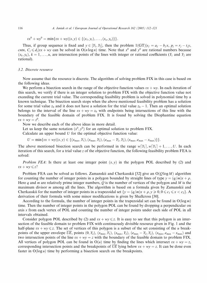
Observe that Df ðyÞ describes the lower envelope for the family of lines fFðf ;jÞðyÞjj ¼ 1; . . . ; qfg. It is a

concave piecewise linear function with at most qf � 1 breakpoints. We are interested only in the part of

Df ðyÞ such that 06 y6 ymax. Denote this part by Df ðyÞ. An example of Df ðyÞ is given in Fig. 2. It is drawnwith a double line.

Similar to the construction of an upper envelope, lower envelope Df ðyÞ can be constructed in

Oðqf log qf Þ time (Boissonnat and Yvinec [4] and Van Hoesel et al. [31]). It may have at most qf þ 1

breakpoints.

Let us count the number of intersection points of the envelopes Df ðyÞ, f ¼ 1; . . . ; g. Since Df ðyÞ is

concave, any line has at most two intersections with Df ðyÞ. Assume without loss of generality that the

groups are numbered in non-increasing order of their cardinalities such that q1 P � � � P qg. The number of

intersection points of the envelopes D2ðyÞ and D1ðyÞ is at most 2q2 because each segment of D2ðyÞ ‘‘pro-duces’’ at most two intersections with D1ðyÞ. The number of intersection points of D3ðyÞ and D1ðyÞ [ D2ðyÞis at most 4q3. Continuing in a similar way, the number of intersection points of DgðyÞ and

D1ðyÞ [ � � � [ Dg�1ðyÞ is at most 2ðg � 1Þqg. Therefore, the total number K of distinct intersection points of

the envelopes Df ðyÞ, f ¼ 1; . . . ; g, can be estimated as

K 6 2q2 þ 4q3 þ � � � þ 2ðg � 1Þqg 6 2ðg � 1Þn:
These distinct intersection points are the only points where the group sequence ðGf1 ;Gf2 ; . . . ;GfgÞ such
that, Df1ðyÞ6Df2ðyÞ6 � � � 6DfgðyÞ can change. Number all these points such that y1 < � � � < yK . Thenumbering can be performed in OðK logKÞ ¼ Oðgn log nÞ time.

Set y0 ¼ 0 and yKþ1 ¼ ymax. For each interval ½yl; ylþ1�, l ¼ 0; . . . ;K, find group sequence Sl ¼ðGf l

1;Gfl

2; . . . ;Gf lg

Þ such that Dfl1ðylÞ6Df l

2ðylÞ6 � � � 6Df lg

ðylÞ.Since the breakpoints of the lower envelope Df are arranged in the increasing or decreasing order of y,

values Df ðylÞ, l ¼ 0; 1; . . . ;K, can be calculated in OðminfK; qF gÞ ¼ OðgnÞ time. All values Df ðylÞ, f ¼1; . . . ; g, l ¼ 0; 1; . . . ;K, can be calculated in Oðg2nÞ time. Therefore, group sequences Sl, l ¼ 0; 1; . . . ;K,can be found in Oðgnminfg; log ngÞ time.

Fig. 2. An example of the envelope Df ðyÞ.


For l ¼ 0; 1; . . . ;K, solve problem FIX with y 2 ½yl; ylþ1� and fixed group sequence Sl. Let ðxðlÞ; yðlÞÞdenote optimal resource values for this problem. Optimal values x� and y� and corresponding group se-

quence for the original problem can be found from

vx� þ wy� ¼ minfvxðlÞ þ wyðlÞjl ¼ 0; 1; . . . ;Kg:
Values x� and y� are rational if the resource is continuously divisible and they are integer if the resource is
discrete.

It remains to show how to find intersection points of the envelopes Df ðyÞ ¼ 1; . . . ; g. This can be done in

Oðn2Þ time by checking whether each segment of one envelope intersects with each segment of the other

envelopes.

To solve the original problem, we first find in Oðn2Þ time the intersection points y1; . . . ; yK , K 6 2ðg � 1Þn,then construct in Oðgnminfg; log ngÞ time group sequences Sl, l ¼ 0; 1; . . . ;K, and finally solve K problems

FIX in Oðgn2 log nÞ and Oðgn2 log2 maxfn;maxj ftjg; v;w; xmax; ymaxgÞ time if the resource is continuously

divisible and discrete, respectively.

5. Fixed processing times or setup times

It might be interesting to solve special cases when either setup times are fixed or job processing times arefixed.

Assume that the job processing times are all fixed. Then we can calculate group deadlines Df ,

f ¼ 1; . . . ; g, according to (4). It will require OðnÞ time. Number groups such that D1 6 � � � 6Dg. Group

sequence ðG1; . . . ;GgÞ is optimal. Recall that the jobs ðf ; jÞ are numbered in the earliest deadline order in

each group. To solve the special case, it remains to find minimum value of x such that 06 x6 xmax and,

according to (1) and (2),

Af � Bf xþXf�1

h¼1

Xqhi¼1

pðh;iÞ þXji¼1

pðf ;iÞ 6 dðf ;jÞ; j ¼ 1; . . . ; qf ; f ¼ 1; . . . ; g:

From latter inequalities, we obtain

xP max Af

(þXf�1

h¼1

Xqhi¼1

pðh;iÞ þXji¼1

pðf ;iÞ � dðf ;jÞ

!,Bf jj ¼ 1; . . . ; qf ; f ¼ 1; . . . ; g

)¼ M :

Value M can be found in OðnÞ time. If the resource is discrete, set M to be equal to dMe. If M > xmax, then

the problem has no feasible solution. Otherwise, x� ¼ maxf0;Mg is the optimal value of x. Thus, theproblem can be solved in Oðn log nÞ time if all job processing times are fixed.

Now assume that the setup times are all fixed. As in the previous section, we can find the intersection

points y1; . . . ; yK of the envelopes Df ðyÞ, f ¼ 1; . . . ; g, construct group sequences Sl, l ¼ 0; 1; . . . ;K, andsolve K problems FIX.

Since setup times are all fixed, problem FIX with group sequence Sl :¼ ðGl; . . . ;GgÞ and restriction

y 2 ½Y1; Y2� allows an easier solution. According to (1) and (2), we must have

Xfh¼1

sh þ Rf�1 þ Rjf � ðTf�1 þ T j

f Þy6 dðf ;jÞ; j ¼ 1; . . . ; qf ; f ¼ 1; . . . ; g;

from where we obtain

yP maxXfh¼1

sh

(þ Rf�1 þ Rj

f � dðf ;jÞ

!,ðTf�1 þ T j

f Þj j ¼ 1; . . . ; qf ; f ¼ 1; . . . ; g

)¼ Z:


Value Z can be found in OðnÞ time. If the resource is discrete, set Z and Y1 to be equal to dZe and dY1e,respectively. If Z > Y2, then problem FIX has no feasible solution. Otherwise, yðlÞ ¼ maxfY1; Zg is the

optimal value of y for the considered problem FIX and y� ¼ minfyðlÞjl ¼ 1; . . . ;Kg is the optimal value of yfor the original problem when setup times are all fixed. In this case, we do not need to construct upper

envelopes and the overall time complexity reduces to Oðgn2Þ.

6. Conclusions

We have shown how to solve the problem 1ðGTÞjsf ¼ af � bf x, pj ¼ rj � tjy, Cj 6 djjvxþ wy in poly-

nomial time by using geometric techniques.

Further research can be undertaken to investigate the problem in which the resource values are not

uniform with respect to different jobs or groups, or the nature of the resources is different, for example, the

resource for setups is continuous and that for the jobs is discrete.

Another interesting extension of the model is to allow the groups to be partitioned into subgroups, each

preceded by the corresponding setup time. This model can provide a better solution when the job deadlinescannot be satisfied if no group splitting is allowed.

References

[1] A.V. Aho, J.E. Hopcroft, J.D. Ullman, The Design and Analysis of Computer Algorithms, Addison-Wesley, Reading, MA, 1974.

[2] D. Biskup, H. Jahnke, Common due date assignment for scheduling on a single machine with jointly reducible processing times,

International Journal of Production Economics 69 (2001) 317–322.

[3] J. Blazewicz, K.H. Ecker, E. Pesch, G. Schmidt, J. Weglarz, Scheduling Computer and Manufacturing Processes, Springer, Berlin,

1996.

[4] J.D. Boissonnat, M. Yvinec, Computational Geometry, Cambridge University Press, Cambridge, 1998.

[5] T.C.E. Cheng, Z.-L. Chen, C.L. Li, B.M.T. Lin, Single machine scheduling to minimize the sum of compression and late costs,

Naval Research Logistics 45 (1998) 67–82.

[6] T.C.E. Cheng, A. Janiak, Resource optimal control in single-machine scheduling with completion time constraints, IEEE

Transactions on Automatic Control 39 (1994) 1243–1246.

[7] T.C.E. Cheng, M.Y. Kovalyov, Single machine batch scheduling with deadlines and resource dependent processing times,

Operations Research Letters 17 (1995) 243–249.

[8] T.C.E. Cheng, A. Janiak, M.Y. Kovalyov, Single machine batch scheduling with resource dependent setup and processing times,

European Journal of Operational Research 135 (2001) 177–183.

[9] Z.L. Chen, Q. Lu, G. Tang, Single machine scheduling with discretely controllable processing times, Operations Research Letters

21 (1997) 69–76.

[10] T.C.E Cheng, C. Oguz, X.D Qi, Due-date assignment and single machine scheduling with compressible processing times,

International Journal of Production Economics 43 (1996) 29–35.

[11] R.L. Graham, E.L Lawler, J.K. Lenstra, A.H.G. Rinnooy Kan, Optimization and approximation in deterministic machine

scheduling: A survey, Annals of Discrete Mathematics 5 (1979) 287–326.

[12] A. Gunasekaran, R. McNeil, R. McGaughey, T. Ajasa, Experiences of a small to medium size enterprise in the design and

implementation of manufacturing cells, International Journal of Computer Integrated Manufacturing 14 (2001) 212–223.

[13] G.C. Hadjinicola, K. Ravi Kumar, Cellular manufacturing at champion irrigation products, International Journal of Operations

and Production Management 13 (1993) 53–61.

[14] I. Ham, K. Hitomy, T. Yoshida, Group Technology: Applications to Production Management, Kluwer-Nijhoff, Boston, 1985.

[15] A. Janiak, Time-optimal control in a single machine problem with resource constraints, Automatica 22 (1986) 745–747.

[16] A. Janiak, Single machine scheduling problem with a common deadline and resource dependent release dates, European Journal

of Operational Research 53 (1991) 317–325.

[17] A. Janiak, M.Y. Kovalyov, Single machine group scheduling with ordered criteria, Annals of Operations Research 57 (1995) 191–

201.

[18] A. Janiak, M.Y. Kovalyov, Single machine scheduling with deadlines and resource dependent processing times, European Journal

of Operational Research 94 (1996) 284–291.


[19] A. Janiak, Y.M. Shafransky, A.V. Tuzikov, Sequencing with ordered criteria, precedence and group technology constraints,

Informatica 12 (2001) 61–88.

[20] A. Janiak, M.-C. Portmann, Minimization of the maximum lateness in single machine scheduling with release dates and additional

resources, Informatica 12 (2001) 61–88.

[21] M.Y. Kovalyov, A.V. Tuziikov, Group sequencing subject to precedence constraints, Applied Mathematics and Computer

Science 4 (1994) 635–641.

[22] C.L Li, E.G. Sewell, T.C.E. Cheng, Scheduling to minimize release-time resource consumption and tardiness penalties, Naval

Research Logistics 42 (1994) 946–966.

[23] M.M. Liaee, H. Emmons, Scheduling families of jobs with setup times, International Journal of Production Economics 51 (1997)

165–176.

[24] Z. Liu, W. Yu, Minimizing the number of late jobs under the group technology assumption, Journal of Combinatorial

Optimization 3 (1999) 5–15.

[25] S.P. Mitrofanov, Scientific principles of group technology, translated by E. Harris, Yorkshire, National Lending Library, 1966.

[26] H. Opitz, A Classification System to Describe Workpieces: Parts I and II, Pergamon, Oxford, 1970.

[27] V.A. Petrov, Flowline Group Production Planning, Business Publications, London, 1966.

[28] C.N. Potts, M.Y. Kovalyov, Scheduling with batching: A review, European Journal of Operational Research 120 (2000) 228–249.

[29] C.N. Potts, L.N. Van Wassenhove, Integrating scheduling with batching and lot-sizing: A review of algorithms and complexity,

Journal of the Operational Research Society 43 (1991) 395–406.

[30] D.F. Shallcross, A polynomial algorithm for a one machine batching problem, Operations Research Letters 11 (1992) 213–218.

[31] S. Van Hoesel, A. Wagelmans, B. Moerman, Using geometric techniques to improve dynamic programming algorithms for the

economic lot-sizing problem and extensions, European Journal of Operational Research 75 (1994) 312–331.

[32] L.Y. Zamanskii, V.L. Cherkasskii, A formula for finding the number of integer points under a straight line and its applications (in

Russian), Economika i Matematicheskie Metodi 20 (1984) 1132–1138.

[33] M.V. Tatikonda, U. Wemmerlv, Adoption and implementation of group technology classification and coding systems: Insights

from seven case studies, International Journal of Production Research 30 (1992) 2087–2110.

[34] T. Yoshida, N. Nakamura, K. Hitomi, A study of production scheduling: Optimization of group scheduling on a single

production stage, Transactions of the Japanese Society of Mechanical Engineers 39 (1973) 1993–2003.

[35] U. Wemmerlv, N.L. Hyer, Cellular manufacturing in the US industry, a survey of current practices, International Journal of

Production Research 27 (1989) 1511–1530.