Sublinear-time algorithms∗

Artur Czumaj† Christian Sohler‡

Abstract

In this paper we survey recent advances in the area of sublinear-time algorithms.

1 Introduction

THe area ofsublinear-time algorithmsis a new rapidly emerging area of computer science. Ithas its roots in the study of massive data sets that occur moreand more frequently in var-

ious applications. Financial transactions with billions of input data and Internet traffic analyses(Internet traffic logs, clickstreams, web data) are examples of modern data sets that show unprece-dented scale. Managing and analyzing such data sets forces us to reconsider the traditional notionsof efficient algorithms: processing such massive data sets in more than linear time is by far tooexpensive and often even linear time algorithms may be too slow. Hence, there is the desire todevelop algorithms whose running times are not only polynomial, but in fact aresublinearin n.

Constructing a sublinear time algorithm may seem to be an impossible task since it allows oneto read only a small fraction of the input. However, in recentyears, we have seen development ofsublinear time algorithms for optimization problems arising in such diverse areas as graph theory,geometry, algebraic computations, and computer graphics.Initially, the main research focus hasbeen on designing efficient algorithms in the framework ofproperty testing(for excellent surveys,see [26, 30, 31, 40, 49]), which is an alternative notion of approximation for decision problems.But more recently, we see some major progress in sublinear-time algorithms in the classical modelof randomized and approximation algorithms. In this paper,we survey some of the recent advancesin this area. Our main focus is on sublinear-time algorithmsfor combinatorial problems, especiallyfor graph problems and optimization problems in metric spaces.

Our goal is to give a flavor of the area of sublinear-time algorithms. We focus on the mostrepresentative results in the area and we aim to illustrate main techniques used to design sublinear-time algorithms. Still, many of the details of the presentedresults are omitted and we recommend

∗Research supported in part by NSF ITR grant CCR-0313219 and NSF DMS grant 0354600.†Department of Computer Science, New Jersey Institute of Technology and Department of Computer Science,

University of Warwick. Email: aczumaj@acm.org.‡Department of Computer Science, Rutgers University and Heinz Nixdorf Institute, University of Paderborn.

Email: csohler@uni-paderborn.de.

the readers to follow the original works. We also do not aim tocover the entire area of sublinear-time algorithms, and in particular, we do not discuss property testing algorithms [26, 30, 31, 40,49], even though this area is very closely related to the research presented in this survey.

Organization. We begin with an introduction to the area and then we give somesublinear-timealgorithms for a basic problem in computational geometry [14]. Next, we present recent sublinear-time algorithms for basic graph problems: approximating the average degree in a graph [25, 34] andestimating the cost of a minimum spanning tree [15]. Then, wediscuss sublinear-time algorithmsfor optimization problems in metric spaces. We present the main ideas behind recent algorithmsfor estimating the cost of minimum spanning tree [19] and facility location [10], and then wediscuss the quality of random sampling to obtain sublinear-time algorithms for clustering problems[20, 46]. We finish with some conclusions.

2 Basic Sublinear Algorithms

The concept of sublinear-time algorithms is known for a verylong time, but initially it has beenused to denote “pseudo-sublinear-time” algorithms, whereafter an appropriatepreprocessing, analgorithm solves the problem in sublinear-time. For example, if we have a set ofn numbers, thenafter anO(n log n) preprocessing (sorting), we can trivially solve a number ofproblems involvingthe input elements. And so, if the after the preprocessing the elements are put in a sorted array,then inO(1) time we can find thekth smallest element, inO(log n) time we can test if the inputcontains a given elementx, and also inO(log n) time we can return the number of elements equalto a given elementx. Even though all these results are folklore, this is not whatwe call nowadaysa sublinear-time algorithm.

In this survey, our goal is to study algorithms for which the input is taken to be in any standardrepresentation and with no extra assumptions. Then, an algorithm does not have to read the entireinput but it may determine the output by checking only a subset of the input elements. It is easyto see that for many natural problems it is impossible to giveany reasonable answer if not all oralmost all input elements are checked. But still, for some number of problems we can obtain goodalgorithms that do not have to look at the entire input. Typically, these algorithms arerandomized(because most of the problems have a trivial linear-time deterministic lower bound) and they returnonly anapproximatesolution rather than the exact one (because usually, without looking at thewhole input we cannot determine the exact solution). In thissurvey, we present recently developedsublinear-time algorithm for some combinatorial optimization problems.

Searching in a sorted list. It is well-known that if we can store the input in a sorted array, thenwe can solve various problems on the input very efficiently. However, the assumption that the inputarray is sorted is not natural in typical applications. Let us now consider a variant of this problem,where our goal is tosearchfor an elementx in a linked sorted list containingn distinctelements1.

1The assumption that the input elements aredistinct is important. If we allow multiple elements to have the samekey, then the search problem requiresΩ(n) time. To see this, consider the input in which about a half of the elements

2

Here, we assume that then elements are stored in a doubly-linked, each list element has access tothe next and preceding element in the list, and the list is sorted (that is, ifx follows y in the list,theny < x). We also assume that we have access to all elements in the list, which for example,can correspond to the situation that alln list elements are stored in an array (but the array is notsorted and we do not impose any order for the array elements).How can we find whether a givennumberx is in our input or is not?

On the first glace, it seems that since we do not have direct access to the rank of any elementin the list, this problem requiresΩ(n) time. And indeed, if our goal is to design a deterministicalgorithm, then it is impossible to do the search ino(n) time. However, if we allow randomization,then we can complete the search inO(

√n) expected time (and this bound is asymptotically tight).

Let us first sample uniformly at random a setS of Θ(√

n) elements from the input. Since wehave access to all elements in the list, we can select the setS in O(

√n) time. Next, we scan all the

elements inS and inO(√

n) time we can find two elements inS, p andq, such thatp ≤ x < q,and there is no element inS that is betweenp andq. Observe that since the input consist ofndistinct numbers,p andq are uniquely defined. Next, we traverse the input list containing all theinput elements starting atp until we find either the sought keyx or we find elementq.

Lemma 1 The algorithm above completes the search in expectedO(√

n) time. Moreover, noalgorithm can solve this problem ino(

√n) expected time.

Proof. The running time of the algorithm if equal toO(√

n) plus the number of the input elementsbetweenp and q. SinceS containsΘ(

√n) elements, the expected number of input elements

betweenp and q is O(n/|S|) = O(√

n). This implies that the expected running time of thealgorithm isO(

√n).

For a proof of a lower bound ofΩ(√

n) expected time, see, e.g., [14]. ⊓⊔

2.1 Geometry: Intersection of Two Polygons

Let us consider a related problem but this time in a geometricsetting. Given two convex polygonsA andB in R2, each withn vertices, determine if they intersect, and if so, then find a point in theirintersection.

It is well known that this problem can be solved inO(n) time, for example, by observing thatit can be described as a linear programming instance in 2-dimensions, a problem which is knownto have a linear-time algorithm (cf. [24]). In fact, within the same time one can either find a pointthat is in the intersection ofA andB, or find a lineL that separatesA from B (actually, one caneven find a bitangent separating lineL, i.e., a line separatingA andB which intersects with eachof A andB in exactly one point). The question is whether we can obtain abetter running time.

The complexity of this problem depends on the input representation. In the most powerfulmodel, if the vertices of both polygons are stored in an arrayin cyclic order, Chazelle and Dobkin[13] showed that the intersection of the polygons can be determined in logarithmic time. However,a standard geometric representation assumes that the inputis not stored in an array but ratherA

has key 1, another half has key 3, and there is a single elementwith key 2. Then, searching for 2 requiresΩ(n) time.

3

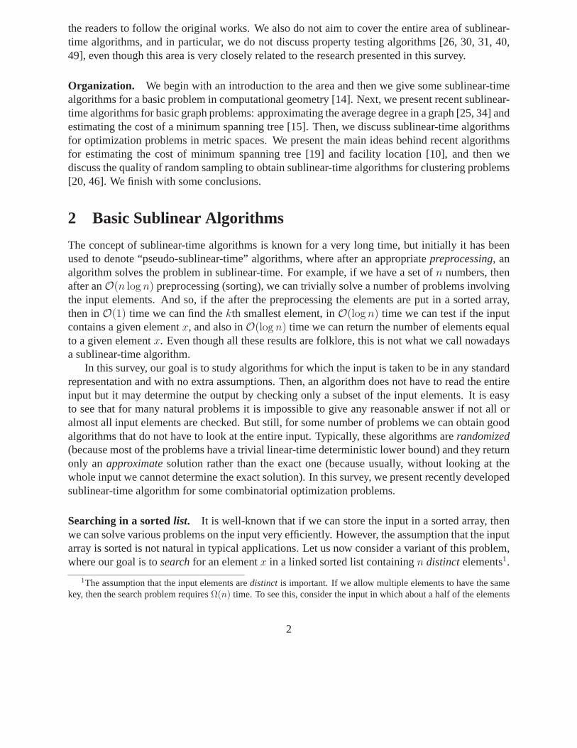
andB are given by their doubly-linked lists of vertices such thateach vertex has as its successorthe next vertex of the polygon in the clockwise order. Can we then test ifA andB intersect?

(a)

C

CB

Aa

b

L

(b)

A C

CA

B

b

aa

L

P

1

Figure 1:(a) Bitangent lineL separatingCA andCB, and (b) the polygonPA.

Chazelle et al. [14] gave anO(√

n)-time algorithm that reuses the approach discussed abovefor searching in a sorted list. Let us first sample uniformly at randomΘ(

√n) vertices from each

A andB, and letCA andCB be the convex hulls of the sample point sets for the polygonsA andB, respectively. Using the linear-time algorithm mentionedabove, inO(

√n) time we can check if

CA andCB intersects. If they do, then the algorithm will get us a pointthat lies in the intersectionof CA andCB, and hence, this point lies also in the intersection ofA andB. Otherwise, letL bethe bitangent separating line returned by the algorithm (see Figure 1 (a)).

Let a andb be the points inL that belong toA andB, respectively. Leta1 anda2 be the twovertices adjacent toa in A. We will define now a new polygonPA. If none ofa1 anda2 is on thesideCA of L the we definePA to be empty. Otherwise, exactly one ofa1 anda2 is on the sideCA

of L; let it bea1. We define polygonPA by walking froma to a1 and then continue walking alongthe boundary ofA until we crossL again (see Figure 1 (b)). In a similar way we define polygonPB. Observe that the expected size of each ofPA andPB is at mostO(

√n).

It is easy to see thatA andB intersects if and only if eitherA intersectsPB or B intersectsPA. We only consider the case of checking ifA intersectsPB. We first determine ifCA intersectsPB. If yes, then we are done. Otherwise, letLA be a bitangent separating line that separatesCA

from PB. We use the same construction as above to determine a subpolygonQA of A that lies onthePB side ofLA. Then,A intersectsPB if and only if QA intersectsPB. SinceQA has expectedsizeO(

√n) and so doesPB, testing the intersection of these two polygons can be done in O(

√n)

expected time. Therefore, by our construction above, we have solved the problem of determiningif two polygons of sizen intersect by reducing it to a constant number of problem instances ofdetermining if two polygons of expected sizeO(

√n) intersect. This leads to the following lemma.

Lemma 2 [14] The problem of determining whether two convexn-gons intersect can be solved inO(

√n) expected time, which is asymptotically optimal.

Chazelle et al. [14] gave not only this result, but they also showed how to apply a similarapproach to design a number of sublinear-time algorithms for some basic geometric problems. Forexample, one can extend the result discussed above to test the intersection of two convex polyhedra

4

in R3 with n vertices inO(√

n) expected time. One can also approximate the volume of ann-vertexconvex polytope to within a relative errorε > 0 in expected timeO(

√n/ε). Or even, for a pair of

two points on the boundary of a convex polytopeP with n vertices, one can estimate the length ofan optimal shortest path outsideP between the given points inO(

√n) expected time.

In all the results mentioned above, the input objects have been represented by a linked struc-ture: either every point has access to its adjacent verticesin the polygon inR2, or the polytope isdefined by a doubly-connected edge list, or so. These input representations are standard in com-putational geometry, but a natural question is whether thisis necessary to achieve sublinear-timealgorithms — what can we do if the input polygon/polytop is represented by a set of points andno additional structure is provided to the algorithm? In such a scenario, it is easy to see that noo(n)-time algorithm can solve exactly any of the problems discussed above. That is, for example,to determine if two polygons withn vertices intersect one needsΩ(n) time. However, still, we canobtain some approximation to this problem, one which is described in the framework ofpropertytesting.

Suppose that we relax our task and instead of determining if two (convex) polytopesA andB inRd intersects, we just want to distinguish between two cases: eitherA andB are intersection-free,or one has to “significantly modify”A andB to make them intersection-free. The definition ofthe notion of “significantly modify” may depend on the application at hand, but the most naturalcharacterization would be to remove at leastε n points inA andB, for an appropriate parameterε(see [18] for a discussion about other geometric characterization). Czumaj et al. [23] gave a simplealgorithm that for anyε > 0, can distinguish between the case whenA andB do not intersect, andthe case when at leastε n points has to be removed fromA andB to make them intersection-free:the algorithm returns the outcome of a test if a random sampleof O((d/ε) log(d/ε)) points fromA intersects with a random sample ofO((d/ε) log(d/ε)) points fromB.

Sublinear-time algorithms: perspective. The algorithms presented in this section should givea flavor of the area and give us the first impression of what do wemean by sublinear-time and whatkind of results one can expect. In the following sections, wewill present more elaborate algorithmsfor various combinatorial problems for graphs and for metric spaces.

3 Sublinear Time Algorithms for Graphs Problems

In the previous section, we introduced the concept of sublinear-time algorithms and we presentedtwo basic sublinear-time algorithms for geometric problems. In this section, we will discusssublinear-time algorithms for graph problems. Our main focus is on sublinear-time algorithmsfor graphs, with special emphasizes on sparse graphs represented by adjacency lists where combi-natorial algorithms are sought.

3.1 Approximating the Average Degree

Assume we have access to the degree distribution of the vertices of an undirected connected graphG = (V,E), i.e., for any vertexv ∈ V we can query for its degree. Can we achieve a good

5

approximation of the average degree inG by looking at a sublinear number of vertices? At firstsight, this seems to be an impossible task. It seems that approximating the average degree isequivalent to approximating the average of a set ofn numbers with values between1 andn − 1,which is not possible in sublinear time. However, Feige [25]proved that one can approximate theaverage degree inO(

√n/ε) time within a factor of2 + ε.

The difficulty with approximating the average of a set ofn numbers can be illustrated with thefollowing example. Assume that almost all numbers in the input set are1 and a few of them aren − 1. To approximate the average we need to approximate how many occurrences ofn − 1 exist.If there is only a constant number of them, we can do this only by looking atΩ(n) numbers in theset. So, the problem is that these large numbers can “hide” inthe set and we cannot give a goodapproximation, unless we can “find” at least some of them.

Why is the problem less difficult, if, instead of an arbitrary set of numbers, we have a set ofnumbers that are the vertex degrees of a graph? For example, we could still have a few vertices ofdegreen−1. The point is that in this case any edge incident to such a vertex can be seen at anothervertex. Thus, even if we do not sample a vertex with high degree we will see all incident edges atother vertices in the graph. Hence, vertices with a large degree cannot “hide.”

We will sketch a proof of a slightly weaker result than that originally proven by Feige [25].Let d denote the average degree inG = (V,E) and letdS denote the random variable for theaverage degree of a setS of s vertices chosen uniformly at random fromV . We will show that ifwe sets ≥ β

√n/εO(1) for an appropriate constantβ, thendS ≥ (1

2− ε) ·d with probability at least

1−ε/64. Additionally, we observe that Markov inequality immediately implies thatdS ≤ (1+ε)·dwith probability at least1 − 1/(1 + ε) ≥ ε/2. Therefore, our algorithm will pick8/ε setsSi, eachof sizes, and output the set with the smallest average degree. Hence,the probability that all ofthe setsSi have too high average degree is at most(1 − ε/2)ε/8 ≤ 1/8. The probability thatone of them has too small average degree is at most8

ε· ε

64= 1/8. Hence, the output value will

satisfy both inequalities with probability at least3/4. By replacingε with ε/2, this will yield a(2 + ε)-approximation algorithm.

Now, our goal is to show that with high probability one does not underestimate the averagedegree too much. LetH be the set of the

√ε n vertices with highest degree inG and letL = V \H

be the set of the remaining vertices. We first argue that the sum of the degrees of the verticesin L is at least(1

2− ε) times the sum of the degrees of all vertices. This can be easily seen by

distinguishing between edges incident to a vertex fromL and edges withinH. Edges incident toa vertex fromL contribute with at least1 to the sum of degrees of vertices inL, which is fineas this is at least1/2 of their full contribution. So the only edges that may cause problems areedges withinH. However, since|H| =

√ε n, there can be at mostε n such edges, which is small

compared to the overall number of edges (which is at leastn − 1, since the graph is connected).Now, letdH be the degree of a vertex with the smallest degree inH. Since we aim at giving a

lower bound on the average degree of the sampled vertices, wecan safely assume that all sampledvertices come from the setL. We know that each vertex inL has a degree between1 anddH . LetXi, 1 ≤ i ≤ s, be the random variable for the degree of theith vertex fromS. Then, it follows

6

from Hoeffding bounds that

Pr[s∑

i=1

Xi ≤ (1 − ε) · E[s∑

i=1

Xi]] ≤ e−

E[Pr

i=1 Xi]·ε2

dH .

We know that the average degree is at leastdH · |H|/n, because any vertex inH has at least degreedH . Hence, the average degree of a vertex inL is at least(1

2− ε) · dH · |H|/n. This just means

E[Xi] ≥ (12−ε)·dH ·|H|/n. By linearity of expectation we getE[

∑si=1 Xi] ≥ s·(1

2−ε)·dH ·|H|/n.

This implies that, for our choice ofs, with high probability we havedS ≥ (12− ε) · d.

Feige showed the following result, which is stronger with respect to the dependence onε.

Theorem 3 [25] UsingO(ε−1 ·√

n/d0) queries, one can estimate the average degree of a graphwithin a ratio of(2 + ε), provided thatd ≥ d0.

Feige also proved thatΩ(ε−1 ·√

n/d) queries are required, whered is the average degree in theinput graph. Finally, any algorithm that uses only degree queries and estimates the average degreewithin a ratio2 − δ for some constantδ requiresΩ(n) queries.

Interestingly, if one can also use neighborhood queries, then it is possible to approximate theaverage degree usingO(

√n/εO(1)) queries with a ratio of(1+ ε), as shown by Goldreich and Ron

[34]. The model for neighborhood queries is as follows. We assume we are given a graph and wecan query for theith neighbor of vertexv. If v has at leasti neighbors we get the correspondingneighbor; otherwise we are told thatv has less thani neighbors. We remark that one can simulatedegree queries in this model withO(log n) queries. Therefore, the algorithm from [34] uses onlyneighbor queries.

For a sketch of a proof, let us assume that we know the setH. Then we can use the followingapproach. We only consider vertices fromL. If our sample contains a vertex fromH we ignoreit. By our analysis above, we know that there are only few edgeswithin H and that we make onlya small error in estimating the number of edges withinL. We loose the factor of two, becausewe “see” edges fromL to H only from one side. The idea behind the algorithm from [34] istoapproximate the fraction of edges fromL to H and add it to the final estimate. This has the effectthat we count any edge betweenL andH twice, canceling the effect that we see it only from oneside. This is done as follows. For each vertexv we sample fromL we take a random set of incidentedges to estimate the fractionλ(v) of its neighbors that is inH. Let λ(v) denote the estimatewe obtain. Then our estimate for the average degree will be

∑v∈S∩L(1 + λ(v)) · d(v)/|S ∩ L|,

whered(v) denotes the degree ofv. If for all vertices we estimateλ(v) within an additive errorof ε, the overall error induced by theλ will be small. This can be achieved with high probabilityqueryingO(log n/ε2) random neighbors. Then the output value will be a(1+ε)-approximation ofthe average degree. The assumption that we knowH can be dropped by taking a set ofO(

√n/ε)

vertices and settingH to be the set of vertices with larger degree than all verticesin this set(breaking ties by the vertex number).

(We remark that the outline of a proof given above is different from the proof in [34].)

Theorem 4 [34] Given the ability to make neighbor queries to the input graphG, there exists analgorithm that makesO(

√n/d0 · ε−O(1)) queries and approximates the average degree inG to

within a ratio of(1 + ε).

7

3.2 Minimum Spanning Trees

One of the most fundamental graph problems is to compute a minimum spanning tree. Since theminimum spanning tree is of size linear in the number of vertices, no sublinear algorithm for sparsegraphs can exists. It is also know that no constant factor approximation algorithm witho(n2) querycomplexity in dense graphs (even in metric spaces) exists [37]. Given these facts, it is somewhatsurprising that it is possible to approximate the cost of a minimum spanning tree in sparse graphs[15] as well as in metric spaces [19] to within a factor of(1 + ε).

In the following we will explain the algorithm for sparse graphs by Chazelle et al. [15]. We willprove a slightly weaker result than in [15]. LetG = (V,E) be an undirected connected weightedgraph with maximum degreeD and integer edge weights from1, . . . ,W. We assume that thegraph is given in adjacency list representation, i.e., for every vertexv there is a list of its at mostD neighbors, which can be accessed fromv. Furthermore, we assume that the vertices are storedin an array such that it is possible to select a vertex uniformly at random. We assume also that thevalues ofD andW are known to the algorithm.

The main idea behind the algorithm is to express the cost of a minimum spanning tree as thenumber of connected components in certain auxiliary subgraphs ofG. Then, one runs a random-ized algorithm to estimate the number of connected components in each of these subgraphs.

To start with basic intuitions, let us assume thatW = 2, i.e., the graph has only edges ofweight1 or 2. LetG(1) = (V,E(1)) denote the subgraph that contains all edges of weight (at most)1 and letc(1) be the number of connected components inG(1). It is easy to see that the minimumspanning tree has to link these connected components by edges of weight2. Since any connectedcomponent inG(1) can be spanned by edges of weight1, any minimum spanning tree ofG hasc(1)−1 edges of weight2 andn−1− (c(1)−1) edges of weight1. Thus, the weight of a minimumspanning tree is

n − 1 − (c(1) − 1) + 2 · (c(1) − 1) = n − 2 + c(1) = n − W + c(1) .

Next, let us consider an arbitrary integer value forW . DefiningG(i) = (V,E(i)), whereE(i) is theset of edges inG with weight at mosti, one can generalize the formula above to obtain that thecostMST of a minimum spanning tree can be expressed as

MST = n − W +W−1∑

i=1

c(i) .

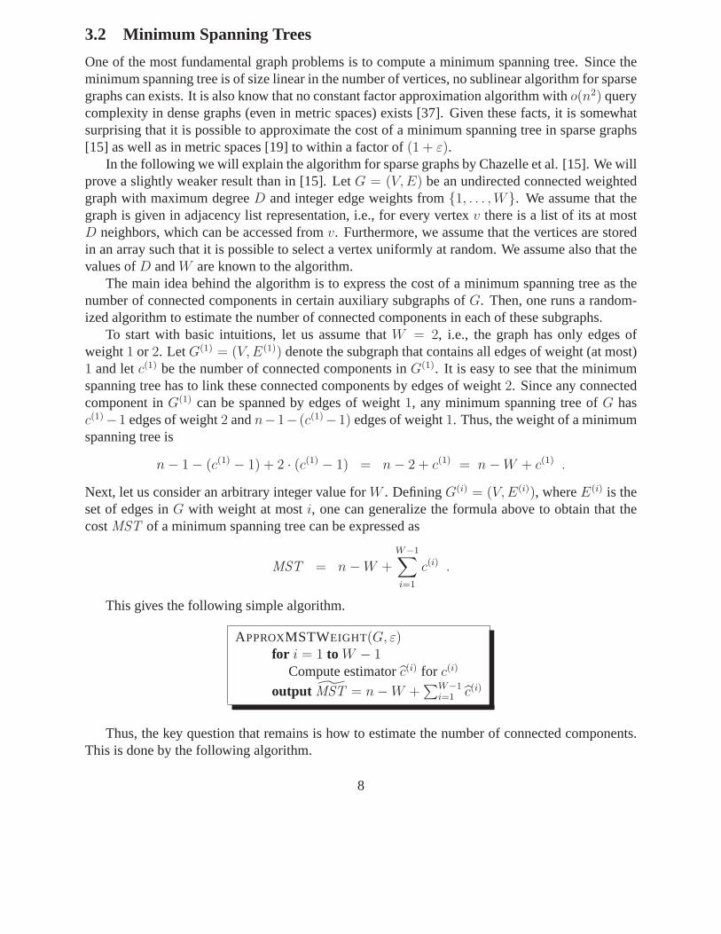
This gives the following simple algorithm.

APPROXMSTWEIGHT(G, ε)for i = 1 to W − 1

Compute estimatorc(i) for c(i)

output MST = n − W +∑W−1

i=1 c(i)

Thus, the key question that remains is how to estimate the number of connected components.This is done by the following algorithm.

8

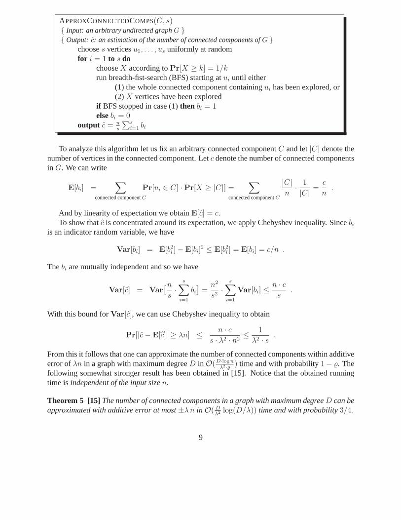
APPROXCONNECTEDCOMPS(G, s) Input: an arbitrary undirected graphG Output: c: an estimation of the number of connected components ofG

chooses verticesu1, . . . , us uniformly at randomfor i = 1 to s do

chooseX according toPr[X ≥ k] = 1/krun breadth-fist-search (BFS) starting atui until either

(1) the whole connected component containingui has been explored, or(2) X vertices have been explored

if BFS stopped in case (1)then bi = 1else bi = 0

output c = ns

∑si=1 bi

To analyze this algorithm let us fix an arbitrary connected componentC and let|C| denote thenumber of vertices in the connected component. Letc denote the number of connected componentsin G. We can write

E[bi] =∑

connected componentC

Pr[ui ∈ C] · Pr[X ≥ |C|] =∑

connected componentC

|C|n

· 1

|C| =c

n.

And by linearity of expectation we obtainE[c] = c.To show thatc is concentrated around its expectation, we apply Chebyshev inequality. Sincebi

is an indicator random variable, we have

Var[bi] = E[b2i ] − E[bi]

2 ≤ E[b2i ] = E[bi] = c/n .

Thebi are mutually independent and so we have

Var[c] = Var[n

s·

s∑

i=1

bi

]=

n2

s2·

s∑

i=1

Var[bi] ≤n · cs

.

With this bound forVar[c], we can use Chebyshev inequality to obtain

Pr[|c − E[c]| ≥ λn] ≤ n · cs · λ2 · n2

≤ 1

λ2 · s .

From this it follows that one can approximate the number of connected components within additiveerror ofλn in a graph with maximum degreeD in O(D·log n

λ2·) time and with probability1− . The

following somewhat stronger result has been obtained in [15]. Notice that the obtained runningtime is independent of the input sizen.

Theorem 5 [15] The number of connected components in a graph with maximum degreeD can beapproximated with additive error at most±λ n in O( D

λ2 log(D/λ)) time and with probability3/4.

9

Now, we can use this procedure with parametersλ = ε/(2W ) and = 14W

in algorithmAPPROXMSTWEIGHT. The probability that at least one call to APPROXCONNECTEDCOMPS isnot within an additive error±λn is at most1/4. The overall additive error is at most±εn/2.Since the cost of the minimum spanning tree is at leastn− 1 ≥ n/2, it follows that the algorithmscomputes inO(D · W 3 · log n/ε2) time a(1 ± ε)-approximation of the weight of the minimumspanning tree with probability at least3/4. In [15], Chazelle et al. proved a slightly stronger resultwhich has running timeindependent of the input size.

Theorem 6 [15] Algorithm APPROXMSTWEIGHT computes a valueMST that with probabilityat least3/4 satisfies

(1 − ε) · MST ≤ MST ≤ (1 + ε) · MST .

The algorithm runs inO(D · W/ε2) time.

The same result also holds whenD is only the average degree of the graph (rather than themaximum degree) and the edge weights are reals from the interval [1,W ] (rather than integers)[15]. Observe that, in particular, for sparse graphs for which the ratio between the maximum andthe minimum weight is constant, the algorithm from [15]runs in constant time!

It was also proved in [15] that any algorithm estimatingMST requiresΩ(D · W/ε2) time.

3.3 Other Sublinear-time Results for Graphs

In this section, our main focus was on combinatorial algorithms for sparse graphs. In particular,we did not discuss a large body of algorithms for dense graphsrepresented in the adjacency matrixmodel. Still, we mention the results of approximating the size of the maximum cut inconstant timefor dense graphs [28, 32], and the more general results aboutapproximating all dense problemsin Max-SNP inconstant time[2, 8, 28]. Similarly, we also have to mention about the existenceof a large body of property testing algorithms for graphs, which in many situations can lead tosublinear-time algorithms for graph problems. To give representative references, in addition tothe excellent survey expositions [26, 30, 31, 40, 49], we want to mention the recent results ontestability of graph properties, as described, e.g., in [3,4, 5, 6, 11, 21, 33, 43].

4 Sublinear Time Approximation Algorithms for Problems inMetric Spaces

One of the most widely considered models in the area of sublinear time approximation algorithmsis thedistance oracle modelfor metric spaces. In this model, the input of an algorithm isa setPof n points in a metric space(P, d). We assume that it is possible to compute the distanced(p, q)between any pair of pointsp, q in constant time. Equivalently, one could assume that the algorithmis given access to then × n distance matrix of the metric space, i.e., we have oracle access to the

10

matrix of a weighted undirected complete graph. Since the full description size of this matrix isΘ(n2), we will call any algorithm witho(n2) running time asublinear algorithm.

Which problems can and cannot be approximated in sublinear time in the distance oraclemodel? One of the most basic problems is to find (an approximation) of the shortest or the longestpairwise distance in the metric space. It turns out that the shortest distance cannot be approximated.The counterexample is a uniform metric (all distances are1) with one distance being set to somevery small valueε. Obviously, it requiresΩ(n2) time to find this single short distance. Hence,no sublinear time approximation algorithm for the shortestdistance problem exists. What aboutthe longest distance? In this case, there is a very simple1

2-approximation algorithm, which was

first observed by Indyk [37]. The algorithm chooses an arbitrary pointp and returns its furthestneighborq. Let r, s be the furthest pair in the metric space. We claim thatd(p, q) ≥ 1

2d(r, s). By

the triangle inequality, we haved(r, p) + d(p, s) ≥ d(r, s). This immediately implies that eitherd(p, r) ≥ 1

2d(r, s) or d(p, s) ≥ 1

2d(r, s). This shows the approximation guarantee.

In the following, we present some recent sublinear-time algorithms for a few optimizationproblems in metric spaces.

4.1 Minimum Spanning Trees

We can view a metric space as a weighted complete graphG. A natural question is whether wecan find out anything about the minimum spanning tree of that graph. As already mentioned in theprevious section, it is not possible to find ino(n2) time a spanning tree in the distance oracle modelthat approximates the minimum spanning tree within a constant factor [37]. However, it is possibleto approximate the weightof a minimum spanning tree within a factor of(1 + ε) in O(n/εO(1))time [19].

The algorithm builds upon the ideas used to approximate the weight of the minimum spanningtree in graphs described in Section 3.2 [15]. Let us first observe that for the metric space problemwe can assume that the maximum distance isO(n/ε) and the shortest distance is1. This can beachieved by first approximating the longest distance inO(n) time and then scaling the problemappropriately. Since by the triangle inequality the longest distance also provides a lower boundon the minimum spanning tree, we can round up to1 all edge weights that are smaller than1.Clearly, this does not significantly change the weight of the minimum spanning tree. Now wecould apply the algorithm APPROXMSTWEIGHT from Section 3.2, but this would not give us ano(n2) algorithm. The reason is that in metric case we have a complete graph, i.e., the averagedegree isD = n − 1, and the edge weights are in the interval[1,W ], whereW = O(n/ε). So, weneed a different approach. In the following we will outline an idea how to achieve a randomizedo(n2) algorithm. To get a near linear time algorithm as in [19] further ideas have to be applied.

The first difference to the algorithm from Section 3.2 is thatwhen we develop a formula for theminimum spanning tree weight, we use geometric progressioninstead of arithmetic progression.Assuming that all edge weights are powers of(1 + ε), we defineG(i) to be the subgraph ofGthat contains all edges of length at most(1 + ε)i. We denote byc(i) the number of connected

11

components inG(i). Then we can write

MST = n − W + ε ·r−1∑

i=0

(1 + ε)i · c(i) , (1)

wherer = log1+ε W − 1.Once we have (1), our approach will be to approximate the number of connected components

c(i) and use formula (1) as an estimator. Although geometric progression has the advantage thatwe only need to estimate the connected components inr = O(log n/ε) subgraphs, the problem isthat the estimator is multiplied by(1 + ε)i. Hence, if we use the procedure from Section 3.2, wewould get an additive error ofε n · (1 + ε)i, which, in general, may be much larger than the weightof the minimum spanning tree.

The basic idea how to deal with this problem is as follows. We will use a different graphtraversal than BFS. Our graph traversal runs only on a subset of the vertices, which are calledrepresentative vertices. Every pair of representative vertices are at distance at leastε · (1 + ε)i

from each other. Now, assume there arem representative vertices and consider the graph inducedby these vertices (there is a problem with this assumption, which will be discussed later). Runningalgorithm APPROXCONNECTEDCOMPS on this induced graph makes an error of±λm, whichmust be multiplied by(1 + ε)i resulting in an additive error of±λ · (1 + ε)i · m. Since them representative vertices have pairwise distanceε · (1 + ε)i, we have a lower boundMST ≥m · ε · (1 + ε)i. Choosingλ = ε2/r would result in a(1 + ε)-approximation algorithm.

Unfortunately, this simple approach does not work. One problem is that we cannot choose arandom representative point. This is because we have no a priori knowledge of the set of repre-sentative points. In fact, in the algorithm the points are chosen greedily during the graph traversal.As a consequence, the decision whether a vertex is a representative vertex or not, depends on thestarting point of the graph traversal. This may also mean that the number of representative verticesin a connected component also depends on the starting point of the graph traversal. However, it isstill possible to cope with these problems and use the approach outlined above to get the followingresult.

Theorem 7 [19] The weight of a minimum spanning tree of ann-point metric space can be ap-proximated inO(n/εO(1)) time to within a(1+ε) factor and with confidence probability at least3

4.

4.1.1 Extensions: Sublinear-time (2 + ε)-approximation of metric TSP and Steiner trees

Let us remark here one direct corollary of Theorem 7. By the well known relationship (see, e.g.,[51]) between minimum spanning trees, travelling salesmantours, and minimum Steiner trees, thealgorithm for estimating the weight of the minimum spanningtree from Theorem 7 immediatelyyieldsO(n/εO(1)) time(2+ε)-approximation algorithms for two other classical problems in metricspaces (or in graphs satisfying the triangle inequality): estimating the weight of thetravellingsalesman tourand theminimum Steiner tree.

12

4.2 Uniform Facility Location

Similarly to the minimum spanning tree problem, one can estimate the cost of themetric uniformfacility location problem inO(n/εO(1)) time [10]. This problem is defined as follows. We aregiven ann-point metric space(P, d). We want to find a subsetF ⊆ P of open facilities such that

|F | +∑

p∈P

d(p, F )

is minimized. Here,d(p, F ) denote the distance fromp to the nearest point inF . It is known thatone cannot find a solution that approximates the optimal solution within a constant factor ino(n2)time [50]. However, it is possible to approximate thecostof an optimal solution within a constantfactor.

The main idea is as follows. Let us denote byB(p, r) the set of points fromP with distance atmostr from p. For eachp ∈ P let rp be the unique value that satisfies

∑

q∈B(p,rp)

(rp − d(p, q)) = 1 .

Then one can show that

Lemma 8 [10]1

4· Opt ≤

∑

p∈P

rp ≤ 6 · Opt ,

whereOpt denotes the cost of an optimal solution to the metric uniformfacility location problem.

Now, the algorithm is based on a randomized algorithm that for a given pointp, estimatesrp towithin a constant factor in timeO(rp ·n · log n) (recall thatrp ≤ 1). Thus, the smallerrp, the fasterthe algorithm. Now, letp be chosen uniformly at random fromP . Then the expected running timeto estimaterp is O(n log n · ∑p∈P rp/n) = O(n log n · E[rp]). We pick a random sample setS ofs = 100 log n/E[rp] points uniformly at random fromP . (The fact that we do not knowE[rp] canbe dealt with by using a logarithmic number of guesses.) Thenwe use our algorithm to computefor eachp ∈ S a valuerp that approximatesrp within a constant factor. Our algorithm outputsns· ∑p∈S rp as an estimate for the cost of the facility location problem.Using Hoeffding bounds

it is easy to prove thatns· ∑

p∈S rp approximates∑

p∈P rp = Opt within a constant factor andwith high probability. Clearly, the same statement is true, when we replace therp values by theirconstant approximationsrp. Finally, we observe that expected running time of our algorithm willbeO(n/εO(1)). This allows us to conclude with the following.

Theorem 9 [10] There exists an algorithm that computes a constant factor approximation to thecost of the metric uniform facility location problem inO(n log2 n) time and with high probability.

13

4.3 Clustering via Random Sampling

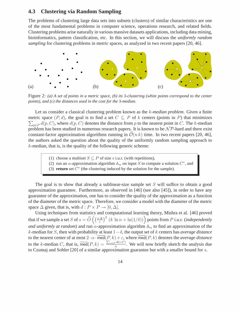
The problems of clustering large data sets into subsets (clusters) of similar characteristics are oneof the most fundamental problems in computer science, operations research, and related fields.Clustering problems arise naturally in various massive datasets applications, including data mining,bioinformatics, pattern classification, etc. In this section, we will discuss theuniformly randomsamplingfor clustering problems in metric spaces, as analyzed in tworecent papers [20, 46].

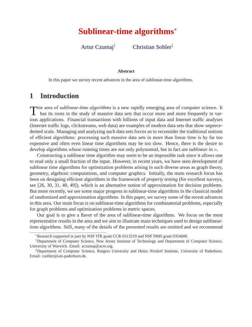
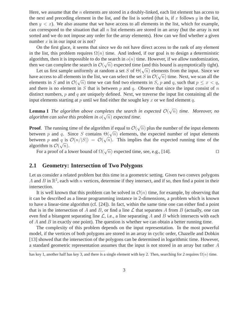
(a) (b) (c)

Figure 2: (a) A set of points in a metric space, (b) its3-clustering (white points correspond to the centerpoints), and (c) the distances used in the cost for the3-median.

Let us consider a classical clustering problem known as thek-median problem. Given a finitemetric space(P, d), the goal is to find a setC ⊆ P of k centers (points inP ) that minimizes∑

p∈P d(p, C), whered(p, C) denotes the distance fromp to the nearest point inC. Thek-medianproblem has been studied in numerous research papers. It is known to beNP-hard and there existconstant-factor approximation algorithms running inO(n k) time. In two recent papers [20, 46],the authors asked the question about the quality of the uniformly random sampling approach tok-median, that is, is the quality of the following generic scheme:

(1) choose a multisetS ⊆ P of sizes i.u.r. (with repetitions),(2) run anα-approximation algorithmAα on inputS to compute a solutionC∗, and(3) return setC∗ (the clustering induced by the solution for the sample).

The goal is to show that already a sublinear-size sample setS will suffice to obtain a goodapproximation guarantee. Furthermore, as observed in [46](see also [45]), in order to have anyguarantee of the approximation, one has to consider the quality of the approximation as a functionof the diameter of the metric space. Therefore, we consider amodel with the diameter of the metricspace∆ given, that is, withd : P × P → [0, ∆].

Using techniques from statistics and computational learning theory, Mishra et al. [46] proved

that if we sample a setS of s = O((

α ∆ε

)2(k ln n + ln(1/δ))

)points fromP i.u.r. (independently

and uniformly at random) and runα-approximation algorithmAα to find an approximation of thek-median forS, then with probability at least1−δ, the output set ofk centers hasaverage distanceto the nearest center of at most2 ·α ·med(P, k)+ ε, wheremed(P, k) denotes theaverage distance

to thek-medianC, that is,med(P, k) =P

v∈P d(v,C)

n. We will now briefly sketch the analysis due

to Czumaj and Sohler [20] of a similar approximation guarantee but with a smaller bound fors.

14

Let Copt denote an optimal set of centers forP and letcost(X,C) be the average cost of the

clustering of setX with center setC, that is,cost(X,C) =P

x∈X d(x,C)

|X|. Notice thatcost(P,Copt) =

med(P, k). The analysis of Czumaj and Sohler [20] is performed in two steps.

(i) We first show that there is a set ofk centersC ⊆ S such thatcost(S,C) is a good approximationof med(P, k) with high probability.

(ii) Next we show that with high probability, every solutionC for P with cost much bigger thanmed(P, k) is either not a feasible solution forS (i.e.,C 6⊆ S) or cost(S,C) ≫ α · med(P, k)(that is, the cost ofC for the sample setS is large with high probability).

SinceS contains a solution with cost at mostc · med(P, k) for some smallc, Aα will computea solutionC∗ with cost at mostα · c · med(P, k). Now we have to prove that no solutionC for Pwith cost much bigger thanmed(P, k) will be returned, or in other words, that ifC is feasible forSthen its cost is larger thanα · c ·med(P, k). But this is implied by (ii). Therefore, the algorithm willnot return a solution with too large cost, and the sampling isa (c · α)-approximation algorithm.

Theorem 10 [20] Let 0 < δ < 1, α ≥ 1, 0 < β ≤ 1 andε > 0 be approximation parameters.

If s ≥ c·αβ

·(k + ∆

ε·β·(α · ln(1/δ) + k · ln

(k ∆ αε β2

)))for an appropriate constantc, then for the

solution set of centersC∗, with probability at least1 − δ it holds the following

cost(V,C∗) ≤ 2 (α + β) · med(P, k) + ε .

To give the flavor of the analysis, we will sketch (a simpler) part (i) of the analysis:

Lemma 11 If s ≥ 3∆α(1+α/β) ln(1/δ)

β·med(P,k)thenPr

[cost(S,C∗) ≤ 2 (α + β) · med(P, k)

]≥ 1 − δ.

Proof. We first show that if we consider the clustering ofS with the optimal set of centersCopt

for P , thencost(S,Copt) is a good approximation ofmed(P, k). The problem with this bound isthat in general, we cannot expectCopt to be contained in the sample setS. Therefore, we have toshow also that the optimal set of centers forS cannot have cost much worse thancost(S,Copt).

Let Xi be the random variable for the distance of theith point inS to the nearest center ofCopt.Then,cost(S,Copt) = 1

s

∑1≤i≤s Xi, and, sinceE[Xi] = med(P, k), we also havemed(P, k) =

1s· E

[∑Xi

]. Hence,

Pr[cost(S,Copt) > (1 + β

α) · med(P, k)

]= Pr

[∑

1≤i≤s

Xi > (1 + βα) · E

[∑

1≤i≤s

Xi

]].

Observe that eachXi satisfies0 ≤ Xi ≤ ∆. Therefore, by Chernoff-Hoeffding bound we obtain:

Pr[ ∑

1≤i≤s

Xi > (1 + β/α) · E[ ∑

1≤i≤s

Xi

]]≤ e−

s·med(P,k)·min(β/α),(β/α)23 ∆ ≤ δ . (2)

This gives us a good bound for the cost ofcost(S,Copt) and now our goal is to get a similarbound for the cost of the optimal set of centers forS. Let C be the set ofk centers inS obtained

15

by replacing eachc ∈ Copt by its nearest neighbor inS. By the triangle inequality,cost(S,C) ≤2 · cost(S,Copt). Hence, multisetS contains a set ofk centers whose cost is at most2 · (1 + β/α) ·med(P, k) with probability at least1 − δ. Therefore, the lemma follows becauseAα returns anα-approximationC∗ of thek-median forS. ⊓⊔

Next, we only state the other lemma that describe part (ii) ofthe analysis of Theorem 10.

Lemma 12 Lets ≥ c·αβ·(k + ∆

ε·β·(α · ln(1/δ) + k · ln

(k ∆ αε β2

)))for an appropriate constantc.

LetC be the set of all sets ofk centersC of P with cost(P,C) > (2 α + 6 β) · med(P, k). Then,

Pr[∃Cb ∈ C : Cb ⊆ S and cost(S,Cb) ≤ 2 (α + β) med(P, k)

]≤ δ . ⊓⊔

Observe that comparing the result from [46] to the result in Theorem 10, Theorem 10 improvesthe sample complexity by a factor of∆ · log n/ε while obtaining a slightly worse approximationratio of 2 (α + β) med(P, k) + ε, instead of2 α med(P, k) + ε as in [46]. However, since thepolynomial-time algorithm with the best known approximation guarantee hasα = 3 + 1

cfor the

running time ofO(nc) time [9], this significantly improves the running time of [46] for all realisticchoices of the input parameters while achieving the same approximation guarantee. As a highlight,Theorem 10 yields a sublinear-time algorithm that in timeO((∆

ε· (k + log(1/δ)))2) — fully inde-

pendent ofn — returns a set ofk centers for which the average distance to the nearest medianis atmostO(med(P, k)) + ε with probability at least1 − δ.

Extensions. The result in Theorem 10 can be significantly improved if we assume the inputpoints are inEuclidean spaceRd. In this case the approximation guarantee can be improved to(α + β) med(P, k) + ε at the cost of increasing the sample size toO(∆·α

ε·β2 · (k d + log(1/δ))).Furthermore, a similar approach as that sketched above can be applied to study similar generic

sample schemes for other clustering problems. As it is shownin [20], almost identical analysislead to sublinear (independent onn) sample complexity for the classicalk-means problem. Also, amore complex analysis can be applied to study the sample complexity for themin-sumk-clusteringproblem[20].

4.4 Other Results

Indyk [37] was the first who observed that some optimization problems in metric spaces can besolved in sublinear-time, that is, ino(n2) time. He presented(1

2− ε)-approximation algorithms for

MaxTSP and the maximum spanning tree problems that run inO(n/ε) time [37]. He also gave a(2+ε)-approximation algorithm for the minimum routing cost spanning tree problem and a(1+ε)approximation algorithm for the average distance problem;both algorithms run inO(n/εO(1)) time.

There is also a number of sublinear-time algorithms for various clustering problems in eitherEuclidean spaces or metric spaces, when the number of clusters is small. For radius (k-center)anddiameter clusteringin Euclidean spaces, sublinear-time property testing algorithms [1, 21]and tolerant testing algorithms [48] have been developed. The first sublinear algorithm for thek-medianproblem was a bicriteria approximation algorithm [37]. This algorithm computes inO(n k)

16

(a) RL

1

1

1

1

1

1

d(e) = 1

(b) RL

1

1

1

1

1

1

d(e) = B

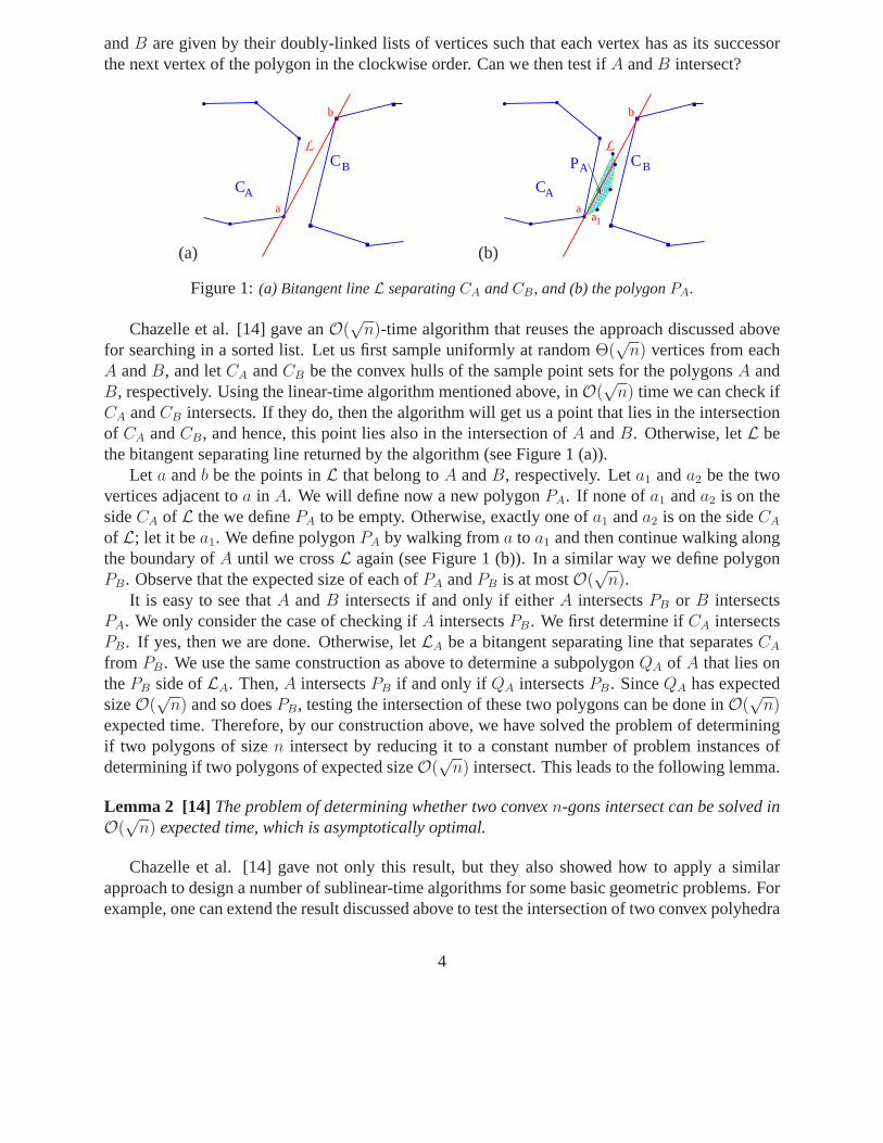
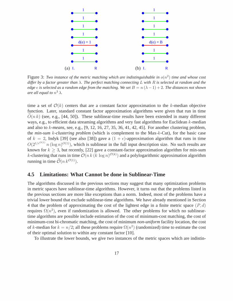
Figure 3:Two instance of the metric matching which are indistinguishable ino(n2) time and whose costdiffer by a factor greater thanλ. The perfect matching connectingL with R is selected at random and theedgee is selected as a random edge from the matching. We setB = n (λ− 1) + 2. The distances not shownare all equal ton3 λ.

time a set ofO(k) centers that are a constant factor approximation to thek-median objectivefunction. Later, standard constant factor approximation algorithms were given that run in timeO(n k) (see, e.g., [44, 50]). These sublinear-time results have been extended in many differentways, e.g., to efficient data streaming algorithms and very fast algorithms for Euclideank-medianand also tok-means, see, e.g., [9, 12, 16, 27, 35, 36, 41, 42, 45]. For another clustering problem,the min-sumk-clustering problem(which is complement to the Max-k-Cut), for the basic caseof k = 2, Indyk [39] (see also [38]) gave a(1 + ǫ)-approximation algorithm that runs in timeO(21/ǫO(1)

n (log n)O(1)), which is sublinear in the full input description size. No such results areknown fork ≥ 3, but recently, [22] gave a constant-factor approximation algorithm for min-sumk-clustering that runs in timeO(n k (k log n)O(k)) and a polylogarithmic approximation algorithmrunning in timeO(n kO(1)).

4.5 Limitations: What Cannot be done in Sublinear-Time

The algorithms discussed in the previous sections may suggest that many optimization problemsin metric spaces have sublinear-time algorithms. However,it turns out that the problems listed inthe previous sections are more like exceptions than a norm. Indeed, most of the problems have atrivial lower bound that exclude sublinear-time algorithms. We have already mentioned in Section4 that the problem of approximating the cost of the lightest edge in a finite metric space(P, d)requiresΩ(n2), even if randomization is allowed. The other problems for which no sublinear-time algorithms are possible include estimation of the costof minimum-cost matching, the cost ofminimum-cost bi-chromatic matching, the cost of minimumnon-uniformfacility location, the costof k-median fork = n/2; all these problems requireΩ(n2) (randomized) time to estimate the costof their optimal solution to within any constant factor [10].

To illustrate the lower bounds, we give two instances of the metric spaces which are indistin-

17

guishable by anyo(n2)-time algorithm for which the cost of the minimum-cost matching in oneinstance is greater thanλ times the one in the other instance (see Figure 3). Consider a metricspace(P, d) with 2n points,n points inL andn points inR. Take a random perfect matchingM between the points inL andR, and then choose an edgee ∈ M at random. Next, define thedistance in(P, d) as follows:

• d(e) is either1 or B, where we setB = n (λ − 1) + 2,

• for anye∗M \ e setd(e∗) = 1, and

• for any other pair of pointsp, q ∈ P not connected by an edge fromM, d(p, q) = n3 λ.

It is easy to see that both instances define properly a metric space(P, d). For such probleminstances, the cost of the minimum-cost matching problem will depend on the choice ofd(e): ifd(e) = B then the cost will ben − 1 + B > nλ, and ifd(e) = 1, then the cost will ben. Hence,any λ-factor approximation algorithm for the matching problem must distinguish between thesetwo problem instances. However, this requires to find if there is an edge of lengthB, and this isknown to require timeΩ(n2), even if a randomized algorithm is used.

5 Conclusions

It would be impossible to present a complete picture of the large body of research known in thearea of sublinear-time algorithms in such a short paper. In this survey, our main goal was to givesome flavor of the area and of the types of the results achievedand the techniques used. For moredetails, we refer to the original works listed in the references.

We did not discuss two important areas that are closely related to sublinear-time algorithms:property testing and data streaming algorithms. For interested readers, we recommend the surveysin [7, 26, 30, 31, 40, 49] and [47], respectively.

References

[1] N. Alon, S. Dar, M. Parnas, and D. Ron. Testing of clustering. SIAM Journal on DiscreteMathematics, 16(3): 393–417, 2003.

[2] N. Alon, W. Fernandez de la Vega, R. Kannan, and M. Karpinski. Random sampling andapproximation of MAX-CSPs.Journal of Computer and System Sciences, 67(2): 212–243,2003.

[3] N. Alon, E. Fischer, M. Krivelevich, M. Szegedy. Efficient testing of large graphs.Combina-torica, 20(4): 451–476, 2000.

[4] N. Alon, E. Fischer, I. Newman, and A. Shapira. A combinatorial characterization of thetestable graph properties: it’s all about regularity.Proceedings of the 38th Annual ACM Sym-posium on Theory of Computing (STOC), 2006.

18

[5] N. Alon and A. Shapira. Every monotone graph property is testable.Proceedings of the 37thAnnual ACM Symposium on Theory of Computing (STOC), pp. 128–137, 2005.

[6] N. Alon and A. Shapira. A characterization of the (natural) graph properties testable with one-sided error.Proceedings of the 46th IEEE Symposium on Foundations of Computer Science(FOCS), pp. 429–438, 2005.

[7] N. Alon and A. Shapira. Homomorphisms in graph property testing - A survey.ElectronicColloquium on Computational Complexity (ECCC), Report No. 85, 2005.

[8] S. Arora, D. R. Karger, and M. Karpinski. Polynomial time approximation schemes for denseinstances ofNP-hard problems. Journal of Computer and System Sciences, 58(1): 193–210,1999.

[9] V. Arya, N. Garg, R. Khandekar, A. Meyerson, K. Munagala, and V. Pandit. Local searchheuristics for k-median and facility location problems.Proceedings of the 33rd Annual ACMSymposium on Theory of Computing (STOC), pp. 21–30, 2001.

[10] M. Badoiu, A. Czumaj, P. Indyk, and C. Sohler. Facility location insublinear time.Proceed-ings of the 32nd Annual International Colloquium on Automata, Languages and Programming(ICALP), pp. 866-877, 2005.

[11] C. Borgs, J. Chayes, L. Lovasz, V. T. Sos, B. Szegedy, and K. Vesztergombi. Graph limits andparameter testing.Proceedings of the 38th Annual ACM Symposium on Theory of Computing(STOC), 2006.

[12] M. Charikar, L. O’Callaghan, and R. Panigrahy. Better streaming algorithms for clusteringproblems.Proceedings of the 35th Annual ACM Symposium on Theory of Computing (STOC),pp. 30–39, 2003.

[13] B. Chazelle and D. P. Dobkin. Intersection of convex objects in two and three dimensions.Journal of the ACM, 34(1): 1–27, 1987.

[14] B. Chazelle, D. Liu, and A. Magen. Sublinear geometric algorithms. SIAM Journal onComputing, 35(3): 627–646, 2006.

[15] B. Chazelle, R. Rubinfeld, and L. Trevisan. Approximating the minimum spanning treeweight in sublinear time.SIAM Journal on Computing, 34(6): 1370–1379, 2005.

[16] K. Chen. Onk-median clustering in high dimensions.Proceedings of the 17th Annual ACM-SIAM Symposium on Discrete Algorithms (SODA), pp. 1177–1185, 2006.

[17] A. Czumaj, F. Ergun, L. Fortnow, A. Magen, I. Newman, R. Rubinfeld, and C. Sohler.Sublinear-time approximation of Euclidean minimum spanning tree.SIAM Journal on Com-puting, 35(1): 91–109, 2005.

19

[18] A. Czumaj and C. Sohler. Property testing with geometric queries. Proceedings of the 9thAnnual European Symposium on Algorithms (ESA), pp. 266–277, 2001.

[19] A. Czumaj and C. Sohler. Estimating the weight of metric minimum spanning trees insublinear-time. Proceedings of the 36th Annual ACM Symposium on Theory of Computing(STOC), pp. 175–183, 2004.

[20] A. Czumaj and C. Sohler. Sublinear-time approximation for clustering via random sampling.Proceedings of the 31st Annual International Colloquium on Automata, Languages and Pro-gramming (ICALP), pp. 396–407, 2004.

[21] A. Czumaj and C. Sohler. Abstract combinatorial programsand efficient property testers.SIAM Journal on Computing, 34(3): 580–615, 2005.

[22] A. Czumaj and C. Sohler. Small space representations for metric min-sumk-clustering andtheir applications. Manuscript, 2006.

[23] A. Czumaj, C. Sohler, and M. Ziegler. Property testing in computational geometry.Proceed-ings of the 8th Annual European Symposium on Algorithms (ESA), pp. 155–166, 2000.

[24] M. Dyer, N. Megiddo, and E. Welzl. Linear programming. In Handbook of Discrete andComputational Geometry, 2nd edition, edited by J. E. Goodman and J. O’Rourke, CRC Press,2004, pp. 999–1014.

[25] U. Feige. On sums of independent random variables with unbounded variance and estimatingthe average degree in a graph.SIAM Journal on Computing, 35(4): 964–984, 2006.

[26] E. Fischer. The art of uninformed decisions: A primer toproperty testing.Bulletin of theEATCS, 75: 97–126, October 2001.

[27] G. Frahling and C. Sohler. Coresets in dynamic geometric data streams.Proceedings of the37th Annual ACM Symposium on Theory of Computing (STOC), pp. 209–217, 2005.

[28] A. Frieze and R. Kannan. Quick approximation to matricesand applications.Combinatorica,19(2): 175–220, 1999.

[29] A. Frieze, R. Kannan, and S. Vempala. Fast Monte-Carlo algorithms for finding low-rankapproximations.Journal of the ACM, 51(6): 1025–1041, 2004.

[30] O. Goldreich. Combinatorial property testing (a survey). In P. Pardalos, S. Rajasekaran, andJ. Rolim, editors,Proceedings of the DIMACS Workshop on Randomization Methodsin Algo-rithm Design, volume 43 ofDIMACS, Series in Discrete Mathetaics and Theoretical ComputerScience, pp. 45–59, 1997. American Mathematical Society, Providence, RI, 1999.

[31] O. Goldreich. Property testing in massive graphs. In J.Abello, P. M. Pardalos, andM. G. C. Resende, editors,Handbook of massive data sets, pp. 123–147. Kluwer AcademicPublishers, 2002.

20

[32] O. Goldreich, S. Goldwasser, and D. Ron. Property testing and its connection to learning andapproximation.Journal of the ACM, 45(4): 653–750, 1998.

[33] O. Goldreich and D. Ron. A sublinear bipartiteness tester for bounded degree graphs.Com-binatorica, 19(3):335–373, 1999.

[34] O. Goldreich and D. Ron. Approximating average parameters of graphs.Electronic Collo-quium on Computational Complexity (ECCC), Report No. 73, 2005.

[35] S. Har-Peled and S. Mazumdar. Coresets fork-means andk-medians and their applications.Proceedings of the 36th Annual ACM Symposium on Theory of Computing (STOC), pp. 291–300, 2004.

[36] S. Har-Peled and A. Kushal. Smaller coresets fork-median andk-means clustering.Proceed-ings of the 21st Annual ACM Symposium on Computational Geometry, pp. 126–134, 2005.

[37] P. Indyk. Sublinear time algorithms for metric space problems. Proceedings of the 31stAnnual ACM Symposium on Theory of Computing (STOC), pp. 428–434, 1999.

[38] P. Indyk. A sublinear time approximation scheme for clustering in metric spaces.Proceedingsof the 40th IEEE Symposium on Foundations of Computer Science(FOCS), pp. 154–159, 1999.

[39] P. Indyk. High-Dimensional Computational Geometry. PhD thesis, Stanford University,2000.

[40] R. Kumar and R. Rubinfeld. Sublinear time algorithms.SIGACT News, 34: 57–67, 2003.

[41] A. Kumar, Y. Sabharwal, and S. Sen. A simple linear time(1 + ε)-approximation algo-rithm for k-means clustering in any dimensions.Proceedings of the 45th IEEE Symposium onFoundations of Computer Science (FOCS), pp. 454–462, 2004.

[42] A. Kumar, Y. Sabharwal, and S. Sen. Linear time algorithms for clustering problems inany dimensions.Proceedings of the 32nd Annual International Colloquium on Automata,Languages and Programming (ICALP), pp. 1374–1385, 2005.

[43] L. Lovasz and B. Szegedy. Graph limits and testing hereditary graphproperties. TechnicalReport, MSR-TR-2005-110, Microsoft Research, August 2005.

[44] R. Mettu and G. Plaxton. Optimal time bounds for approximate clustering.Machine Learn-ing, 56(1-3):35–60, 2004.

[45] A. Meyerson, L. O’Callaghan, and S. Plotkin. Ak-median algorithm with running timeindependent of data size.Machine Learning, 56(1–3): 61–87, July 2004.

[46] N. Mishra, D. Oblinger, and L. Pitt. Sublinear time approximate clustering.Proceedings ofthe 12th Annual ACM-SIAM Symposium on Discrete Algorithms (SODA), pp. 439–447, 2001.

21

[47] S. Muthukrishnan. Data streams: Algorithms and applications. InFoundations and Trends inTheoretical Computer Science, volume 1, issue 2, August 2005.

[48] M. Parnas, D. Ron, and R. Rubinfeld. Tolerant property testing and distance approximation.Electronic Colloquium on Computational Complexity (ECCC), Report No. 10, 2004.

[49] D. Ron. Property testing. In P. M. Pardalos, S. Rajasekaran, J. Reif, and J. D. P. Rolim,editors,Handobook of Randomized Algorithms, volume II, pp. 597–649. Kluwer AcademicPublishers, 2001.

[50] M. Thorup. Quickk-median,k-center, and facility location for sparse graphs.SIAM Journalon Computing, 34(2):405–432, 2005.

[51] V. V. Vazirani. Approximation Algorithms. Springer-Verlag, New York, 2004.

22