Download pdf - Switching In Active Vibration Isolation Systems · includes a passive vibration isolation portion to ... Toward Switching In Active Vibration Isolation ... in active vibration isolation

Switching In Active Vibration Isolation Systems

Internship

H.G. Yegen DC 2010.048

Coach: Dr. Ir. M.F. Heertjes Supervisor: Prof. Dr. H. Nijmeijer Eindhoven University of Technology Department of Mechanical Engineering Systems and Control Master Program Dynamics and Control Group Eindhoven, September 7, 2010

1 TU/e, Department of Mechanical Engineering, Dynamics and Control Group, 2010

Toward Switching In Active Vibration Isolation Systems 2

CONTENTS

Preface ……................................................................................................................................................ 4

Summary……................................................................................................................................................ 6

1 Introduction……..................................................................................................................................... 8

2 Active Vibration Isolation System…….......................................................................................... 12

2.1 Experimental setup……....................................................................................................... 12

2.2 Control design…….................................................................................................................. 13

2.3 Simulink……............................................................................................................................. 16

3 Experimental parameter studies.................................................................................................... 18

3.1 Sensor Calibration ……........................................................................................................ 18

3.2 Switching control parameter studies ........................................................................... 19

3.2.1 Switching length, delta [δ] ……........................................................................ 19

3.2.2 Switching gain, alpha [α] ……........................................................................... 21

3.2.3 Two parameters effect……................................................................................ 24

3.3 Surface fit and Global minimum approach................................................................ 29

4 Conclusions and Recommendations............................................................................................. 32

Bibliography……..................................................................................................................................... 34



Preface

This report, Optimal Switching in Active Vibration Isolation Systems (AVIS), covers the internship study of the author, who is studying within the System and Control master program at the Eindhoven Technical University, under the supervision of Prof. Dr. Henk Nijmeijer. The report is accompanied by a CD-ROM, which contains an electronic version of this report, as well as a presentation, a poster and the demo files of this research.



Summary

In a wide range of industrial applications such as semiconductor instruments and manufacturing machines, the requirement of vibration isolation systems is increasing to obtain precise and repeatable results. Although linear active vibration isolation seems to work properly for the lower frequencies, the performance at higher frequencies is worse than without control. The switching control approach is considered to solve this problem.

The vibration isolation system that is considered in this report is the Active Vibration Isolation System (AVIS) which is developed by IDE Engineering. The AVIS is capable of six degree of-freedom active vibration control and mainly consists of a payload and a chassis which are interconnected by means of four isolator modules but in this report only the (vertical) z-axis will be considered. The goal of switching control in the active vibration isolation systems is to use the controller only incidentally to suppress low-frequency responses and turn off the controller otherwise as to avoid noise amplification. The nonlinear controller has two parameters to tune: the switching gain and the switching length. The effect of these parameters is measured when varied separately or together. The experimental results are further processed to study the effects of the parameters of the switching control. This demonstrates optimal settings in terms of error and control force levels.



CHAPTER 1

INTRODUCTION

Vibration isolation systems have a wide range of applications such as automobiles, buildings, aerospace structures. The necessity of suppressing unwanted vibrations using vibration isolation from different sources, even natural environmental vibration, are increasing because manufacturing of different products becomes more precise [4]. In illustrating the vibration isolation principle, a distinction is made between passive and active vibration isolation. A passive vibration isolation system consists of a spring and damper. The spring is intended to isolate from external vibrations but conserves energy. The damper has to damp the oscillations excited by the system and dissipates energy. An active vibration isolation system includes a passive vibration isolation portion to isolate the load from high frequency noise, and sensors and actuators for active isolation from low-frequency vibration. This mainly involves applying active damping in addition to the marginally passive damping which is presented. Due to that, active isolation systems can operate reliably over a wide range of frequencies.

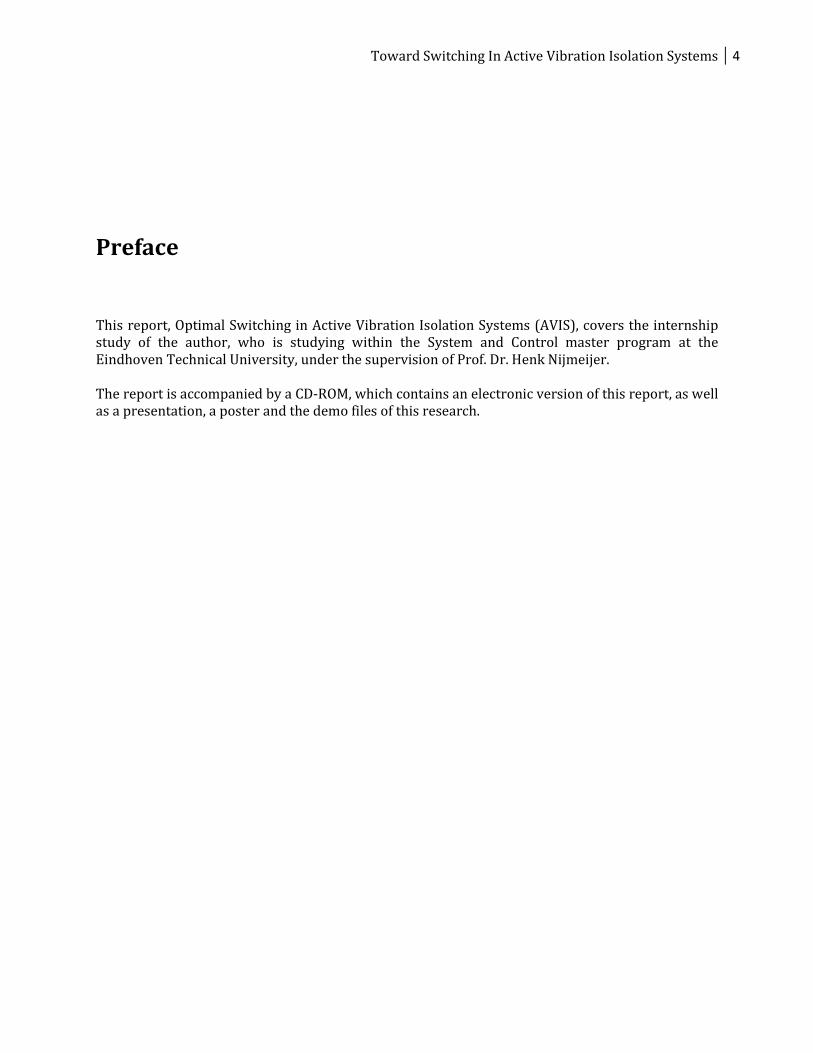
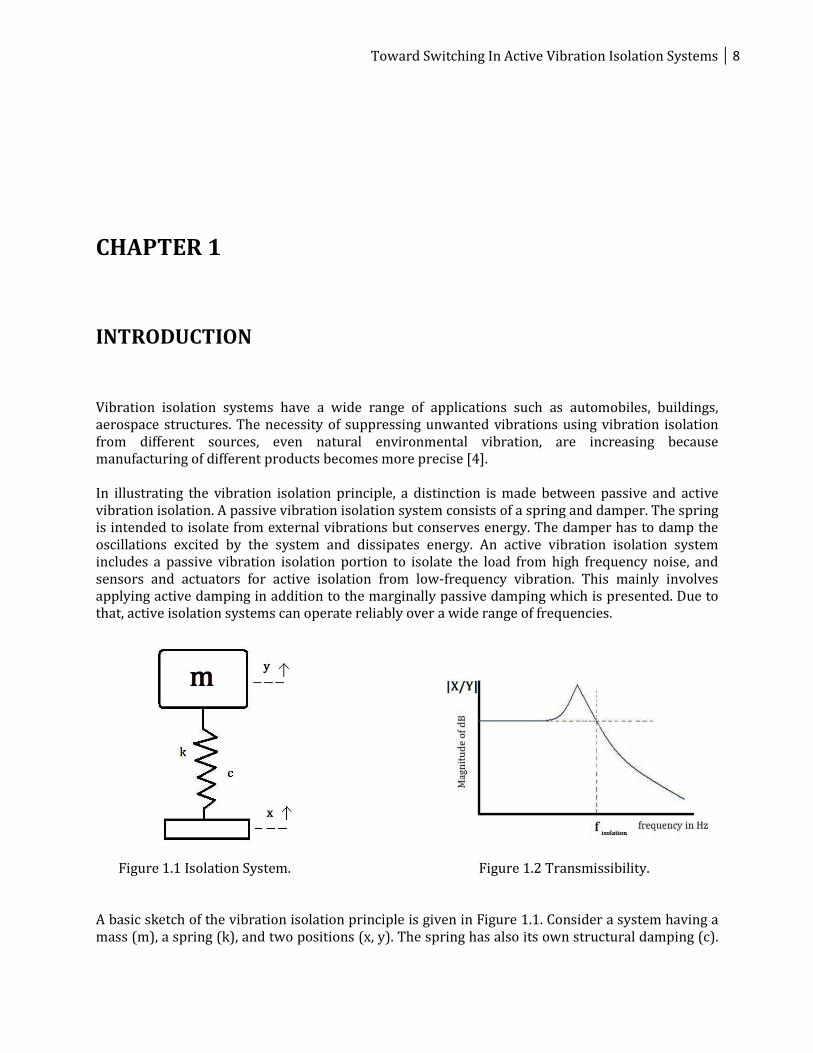
Figure 1.1 Isolation System. Figure 1.2 Transmissibility. A basic sketch of the vibration isolation principle is given in Figure 1.1. Consider a system having a mass (m), a spring (k), and two positions (x, y). The spring has also its own structural damping (c).


Given the motion of the floor represented by x and the motion of the isolated payload represented by y, the isolation transfer between x and y is given by the transmissibility function, which is the transfer function between the displacement of the ground and the displacement of the payload, shown in Figure 1.2. The definition of the transmissibility (1.5) is given below:

Assume (1.1).

Then through Newton’s second law it follows that

(1.2), or using (1.1)

(1.3), which gives

(1.4).

For the magnitude (1.5).

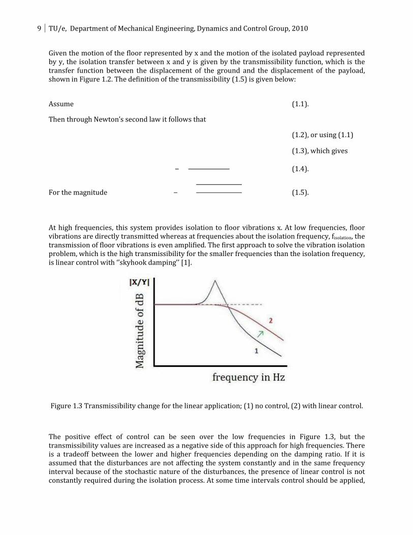
At high frequencies, this system provides isolation to floor vibrations x. At low frequencies, floor vibrations are directly transmitted whereas at frequencies about the isolation frequency, fisolation, the transmission of floor vibrations is even amplified. The first approach to solve the vibration isolation problem, which is the high transmissibility for the smaller frequencies than the isolation frequency, is linear control with ‘’skyhook damping’’ [1].

Figure 1.3 Transmissibility change for the linear application; (1) no control, (2) with linear control.

The positive effect of control can be seen over the low frequencies in Figure 1.3, but the transmissibility values are increased as a negative side of this approach for high frequencies. There is a tradeoff between the lower and higher frequencies depending on the damping ratio. If it is assumed that the disturbances are not affecting the system constantly and in the same frequency interval because of the stochastic nature of the disturbances, the presence of linear control is not constantly required during the isolation process. At some time intervals control should be applied,


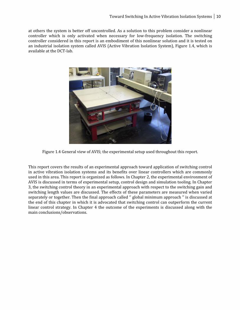
at others the system is better off uncontrolled. As a solution to this problem consider a nonlinear controller which is only activated when necessary for low-frequency isolation. The switching controller considered in this report is an embodiment of this nonlinear solution and it is tested on an industrial isolation system called AVIS (Active Vibration Isolation System), Figure 1.4, which is available at the DCT-lab.

Figure 1.4 General view of AVIS; the experimental setup used throughout this report.

This report covers the results of an experimental approach toward application of switching control in active vibration isolation systems and its benefits over linear controllers which are commonly used in this area. This report is organized as follows. In Chapter 2, the experimental environment of AVIS is discussed in terms of experimental setup, control design and simulation tooling. In Chapter 3, the switching control theory in an experimental approach with respect to the switching gain and switching length values are discussed. The effects of these parameters are measured when varied separately or together. Then the final approach called ‘’ global minimum approach ’’ is discussed at the end of this chapter in which it is advocated that switching control can outperform the current linear control strategy. In Chapter 4 the outcome of the experiments is discussed along with the main conclusions/observations.



CHAPTER 2

ACTIVE VIBRATION ISOLATION SYSTEM

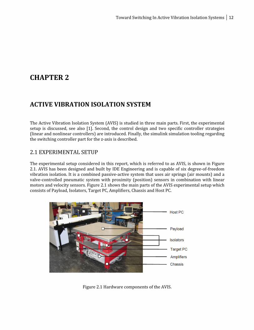
The Active Vibration Isolation System (AVIS) is studied in three main parts. First, the experimental setup is discussed, see also [1]. Second, the control design and two specific controller strategies (linear and nonlinear controllers) are introduced. Finally, the simulink simulation tooling regarding the switching controller part for the z-axis is described. 2.1 EXPERIMENTAL SETUP The experimental setup considered in this report, which is referred to as AVIS, is shown in Figure 2.1. AVIS has been designed and built by IDE Engineering and is capable of six degree-of-freedom vibration isolation. It is a combined passive-active system that uses air springs (air mounts) and a valve-controlled pneumatic system with proximity (position) sensors in combination with linear motors and velocity sensors. Figure 2.1 shows the main parts of the AVIS experimental setup which consists of Payload, Isolators, Target PC, Amplifiers, Chassis and Host PC.

Figure 2.1 Hardware components of the AVIS.


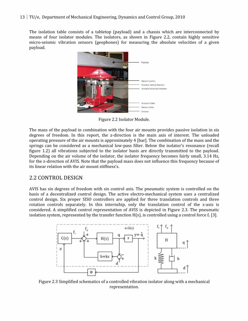
The isolation table consists of a tabletop (payload) and a chassis which are interconnected by means of four isolator modules. The isolators, as shown in Figure 2.2, contain highly sensitive micro-seismic vibration sensors (geophones) for measuring the absolute velocities of a given payload.

Figure 2.2 Isolator Module.

The mass of the payload in combination with the four air mounts provides passive isolation in six degrees of freedom. In this report, the z-direction is the main axis of interest. The unloaded operating pressure of the air mounts is approximately 4 [bar]. The combination of the mass and the springs can be considered as a mechanical low-pass filter. Below the isolator’s resonance (recall figure 1.2) all vibrations subjected to the isolator basis are directly transmitted to the payload. Depending on the air volume of the isolator, the isolator frequency becomes fairly small, 3.14 Hz, for the z-direction of AVIS. Note that the payload mass does not influence this frequency because of its linear relation with the air mount stiffness’s. 2.2 CONTROL DESIGN AVIS has six degrees of freedom with six control axis. The pneumatic system is controlled on the basis of a decentralized control design. The active electro-mechanical system uses a centralized control design. Six proper SISO controllers are applied for three translation controls and three rotation controls separately. In this internship, only the translation control of the z-axis is considered. A simplified control representation of AVIS is depicted in Figure 2.3. The pneumatic isolation system, represented by the transfer function H(s), is controlled using a control force fc [3].

Figure 2.3 Simplified schematics of a controlled vibration isolator along with a mechanical

representation.


A fourth-order isolator model is given by

with m1 = 274.8 kg, m2 = 14.5 kg, b12 = 248.2 Nsm−1, k12 = 44997 Nm−1, b = 831.5 Nsm−1, and k = 190670 Nm−1. The isolation system is subjected to environmental disturbances d (floor vibrations) and fd (acoustic excitations) and a controller force fc. Given the payload vertical velocity , the controller transfer function C(s) from to fc is given by

009-e 009-e

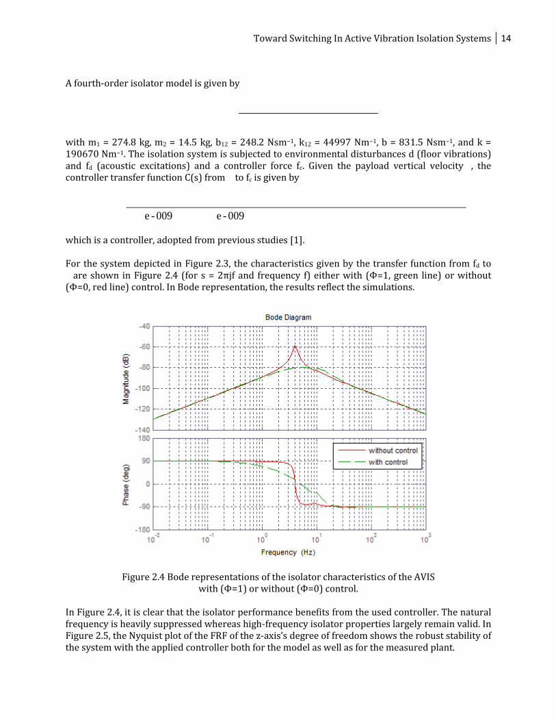
which is a controller, adopted from previous studies [1]. For the system depicted in Figure 2.3, the characteristics given by the transfer function from fd to

are shown in Figure 2.4 (for s = 2πjf and frequency f) either with (Φ=1, green line) or without (Φ=0, red line) control. In Bode representation, the results reflect the simulations.

Figure 2.4 Bode representations of the isolator characteristics of the AVIS with (Φ=1) or without (Φ=0) control.

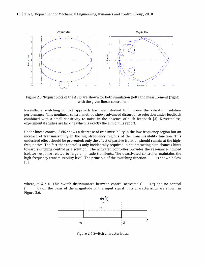
In Figure 2.4, it is clear that the isolator performance benefits from the used controller. The natural frequency is heavily suppressed whereas high-frequency isolator properties largely remain valid. In Figure 2.5, the Nyquist plot of the FRF of the z-axis’s degree of freedom shows the robust stability of the system with the applied controller both for the model as well as for the measured plant.


Figure 2.5 Nyquist plots of the AVIS are shown for both simulation (left) and measurement (right)

with the given linear controller.

Recently, a switching control approach has been studied to improve the vibration isolation performance. This nonlinear control method shows advanced disturbance rejection under feedback combined with a small sensitivity to noise in the absence of such feedback [3]. Nevertheless, experimental studies are lacking which is exactly the aim of this report. Under linear control, AVIS shows a decrease of transmissibility in the low-frequency region but an increase of transmissibility in the high-frequency regions of the transmissibility function. This undesired effect should be prevented; only the effect of passive isolation should remain at the high-frequencies. The fact that control is only incidentally required in counteracting disturbances hints toward switching control as a solution. The activated controller provides the resonance-induced isolator response related to large-amplitude transients. The deactivated controller maintains the high-frequency transmissibility level. The principle of the switching function is shown below [3]:

where, α, δ ≥ 0. This switch discriminates between control activated ( =α) and no control ( 0) on the basis of the magnitude of the input signal . Its characteristics are shown in Figure 2.6.

Figure 2.6 Switch characteristics.


As being the main topic of this report, detailed information about the switching control and its application will be given in Chapter 3 where the effects of the switching gain (alpha [α]) and switching length (delta [δ]) will be investigated experimentally. 2.3 SIMULINK

The experimental environment of AVIS consists of 3 parts: the experimental structure, target computer and host computer. The host computer represents the main computer which has the Matlab and simulink files to control the structure.

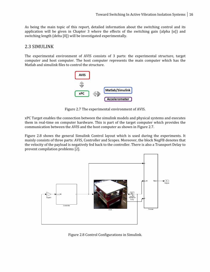
Figure 2.7 The experimental environment of AVIS. xPC Target enables the connection between the simulink models and physical systems and executes them in real-time on computer hardware. This is part of the target computer which provides the communication between the AVIS and the host computer as shown in Figure 2.7. Figure 2.8 shows the general Simulink Control layout which is used during the experiments. It mainly consists of three parts: AVIS, Controller and Scopes. Moreover, the block NegFB denotes that the velocity of the payload is negatively fed back to the controller. There is also a Transport Delay to prevent compilation problems [2].

Figure 2.8 Control Configurations in Simulink.


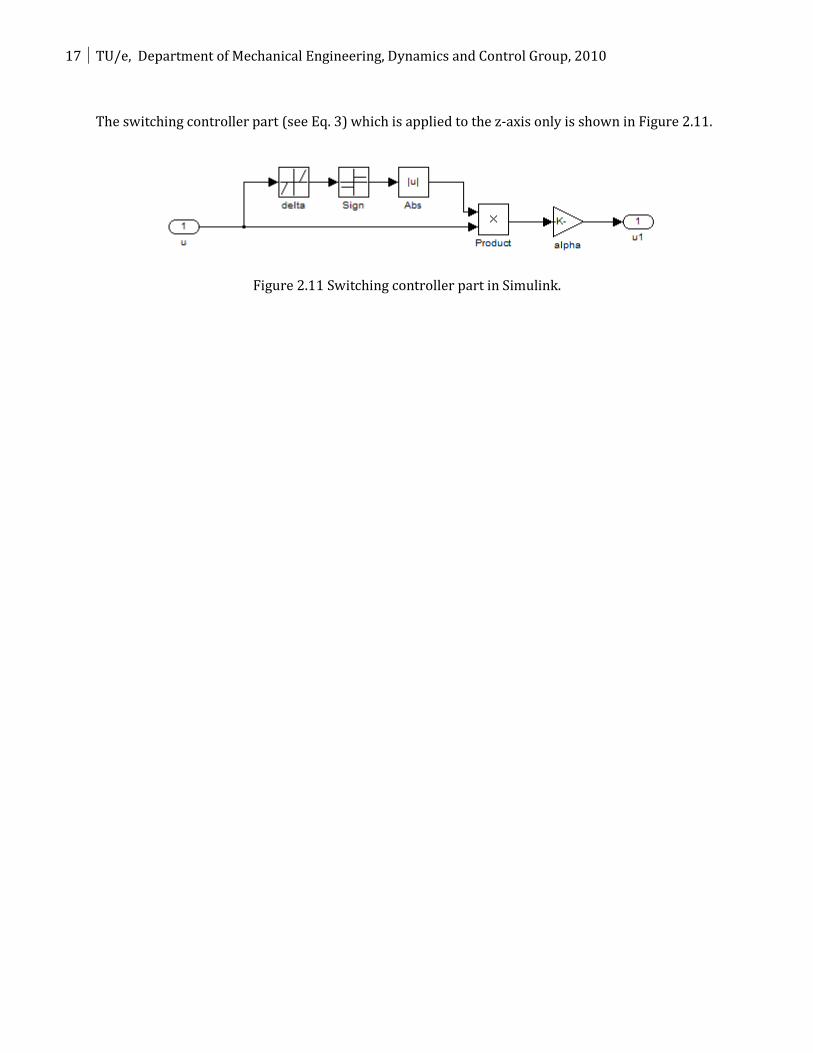
The switching controller part (see Eq. 3) which is applied to the z-axis only is shown in Figure 2.11.

Figure 2.11 Switching controller part in Simulink.


CHAPTER 3

EXPERIMENTAL PARAMETER STUDIES

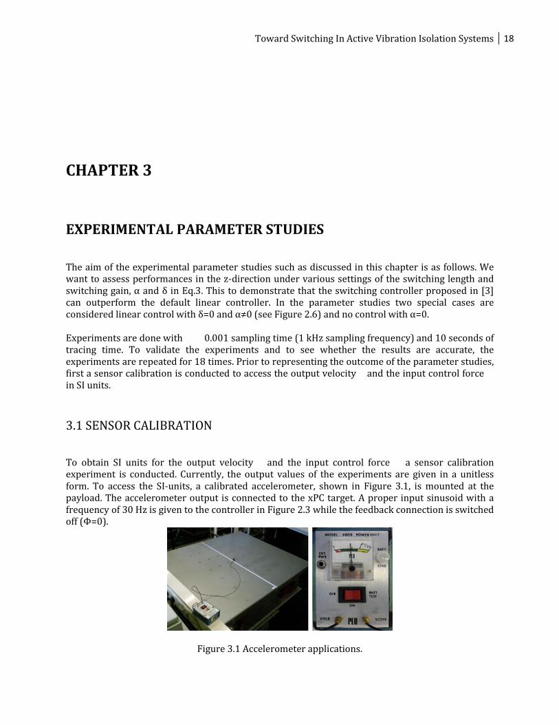
The aim of the experimental parameter studies such as discussed in this chapter is as follows. We want to assess performances in the z-direction under various settings of the switching length and switching gain, α and δ in Eq.3. This to demonstrate that the switching controller proposed in [3] can outperform the default linear controller. In the parameter studies two special cases are considered linear control with δ=0 and α≠0 (see Figure 2.6) and no control with α=0. Experiments are done with 0.001 sampling time (1 kHz sampling frequency) and 10 seconds of tracing time. To validate the experiments and to see whether the results are accurate, the experiments are repeated for 18 times. Prior to representing the outcome of the parameter studies, first a sensor calibration is conducted to access the output velocity and the input control force in SI units. 3.1 SENSOR CALIBRATION To obtain SI units for the output velocity and the input control force a sensor calibration experiment is conducted. Currently, the output values of the experiments are given in a unitless form. To access the SI-units, a calibrated accelerometer, shown in Figure 3.1, is mounted at the payload. The accelerometer output is connected to the xPC target. A proper input sinusoid with a frequency of 30 Hz is given to the controller in Figure 2.3 while the feedback connection is switched off (Φ=0).

Figure 3.1 Accelerometer applications.


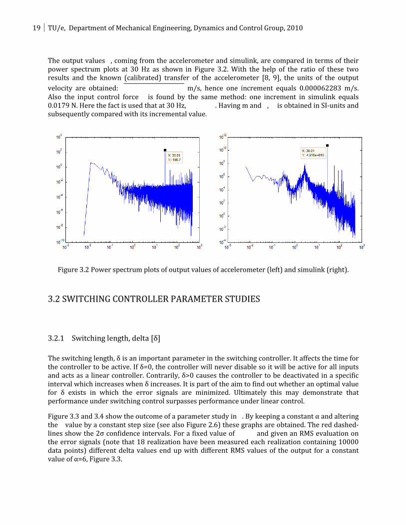
The output values , coming from the accelerometer and simulink, are compared in terms of their power spectrum plots at 30 Hz as shown in Figure 3.2. With the help of the ratio of these two results and the known (calibrated) transfer of the accelerometer [8, 9], the units of the output velocity are obtained: m/s, hence one increment equals 0.000062283 m/s. Also the input control force is found by the same method: one increment in simulink equals 0.0179 N. Here the fact is used that at 30 Hz, . Having m and , is obtained in SI-units and subsequently compared with its incremental value.

Figure 3.2 Power spectrum plots of output values of accelerometer (left) and simulink (right).

3.2 SWITCHING CONTROLLER PARAMETER STUDIES

3.2.1 Switching length, delta [δ]

The switching length, δ is an important parameter in the switching controller. It affects the time for the controller to be active. If δ=0, the controller will never disable so it will be active for all inputs and acts as a linear controller. Contrarily, δ>0 causes the controller to be deactivated in a specific interval which increases when δ increases. It is part of the aim to find out whether an optimal value for δ exists in which the error signals are minimized. Ultimately this may demonstrate that performance under switching control surpasses performance under linear control.

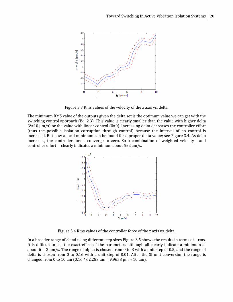
Figure 3.3 and 3.4 show the outcome of a parameter study in . By keeping a constant α and altering the value by a constant step size (see also Figure 2.6) these graphs are obtained. The red dashed-lines show the 2σ confidence intervals. For a fixed value of and given an RMS evaluation on the error signals (note that 18 realization have been measured each realization containing 10000 data points) different delta values end up with different RMS values of the output for a constant value of α=6, Figure 3.3.


Figure 3.3 Rms values of the velocity of the z axis vs. delta.

The minimum RMS value of the outputs given the delta set is the optimum value we can get with the switching control approach (Eq. 2.3). This value is clearly smaller than the value with higher delta (δ=10 µm/s) or the value with linear control (δ=0). Increasing delta decreases the controller effort (thus the possible isolation corruption through control) because the interval of no control is increased. But now a local minimum can be found for a proper delta value; see Figure 3.4. As delta increases, the controller forces converge to zero. So a combination of weighted velocity and controller effort clearly indicates a minimum about δ≈2 µm/s.

Figure 3.4 Rms values of the controller force of the z axis vs. delta.

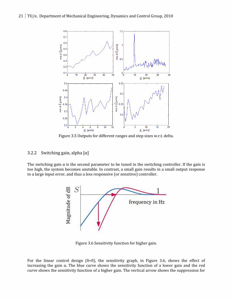
In a broader range of δ and using different step sizes Figure 3.5 shows the results in terms of rms. It is difficult to see the exact effect of the parameters although all clearly indicate a minimum at about δ 3 µm/s. The range of alpha is chosen from 0 to 8 with a unit step of 0.5, and the range of delta is chosen from 0 to 0.16 with a unit step of 0.01. After the SI unit conversion the range is changed from 0 to 10 µm (0.16 * 62.283 µm = 9.9653 µm ≈ 10 µm).


Figure 3.5 Outputs for different ranges and step sizes w.r.t. delta.

3.2.2 Switching gain, alpha [α]

The switching gain α is the second parameter to be tuned in the switching controller. If the gain is too high, the system becomes unstable. In contrast, a small gain results in a small output response to a large input error, and thus a less responsive (or sensitive) controller.

Figure 3.6 Sensitivity function for higher gain.

For the linear control design (δ=0), the sensitivity graph, in Figure 3.6, shows the effect of increasing the gain α. The blue curve shows the sensitivity function of a lower gain and the red curve shows the sensitivity function of a higher gain. The vertical arrow shows the suppression for


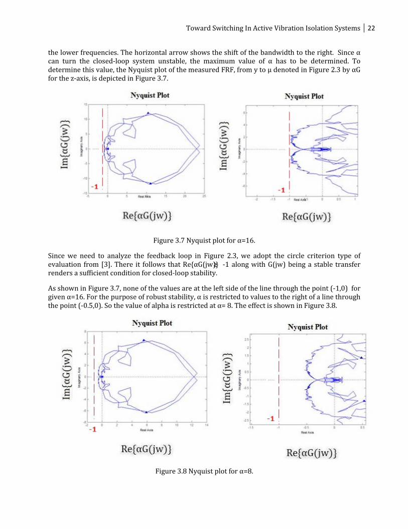
the lower frequencies. The horizontal arrow shows the shift of the bandwidth to the right. Since α can turn the closed-loop system unstable, the maximum value of α has to be determined. To determine this value, the Nyquist plot of the measured FRF, from y to µ denoted in Figure 2.3 by αG for the z-axis, is depicted in Figure 3.7.

Figure 3.7 Nyquist plot for α=16.

Since we need to analyze the feedback loop in Figure 2.3, we adopt the circle criterion type of evaluation from [3]. There it follows that Re{αG(jw)}≥ -1 along with G(jw) being a stable transfer renders a sufficient condition for closed-loop stability.

As shown in Figure 3.7, none of the values are at the left side of the line through the point (-1,0) for given α=16. For the purpose of robust stability, α is restricted to values to the right of a line through the point (-0.5,0). So the value of alpha is restricted at α= 8. The effect is shown in Figure 3.8.

Figure 3.8 Nyquist plot for α=8.


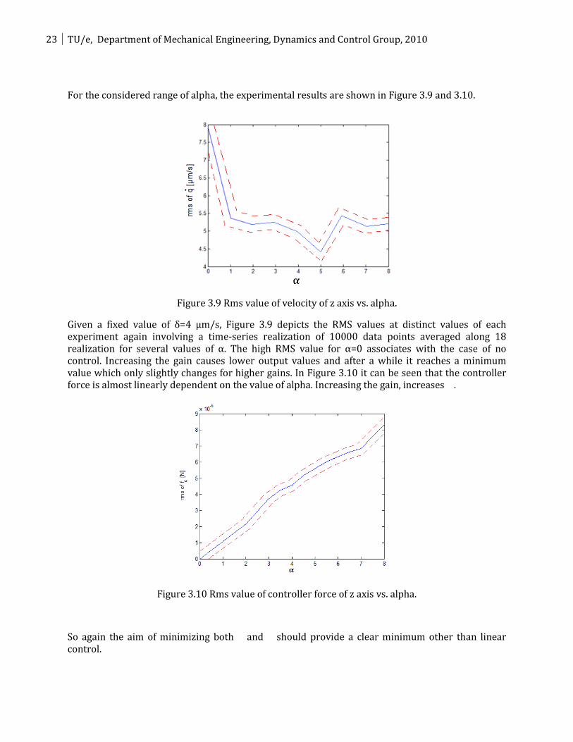
For the considered range of alpha, the experimental results are shown in Figure 3.9 and 3.10.

Figure 3.9 Rms value of velocity of z axis vs. alpha.

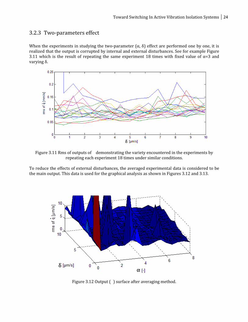
Given a fixed value of δ=4 µm/s, Figure 3.9 depicts the RMS values at distinct values of each experiment again involving a time-series realization of 10000 data points averaged along 18 realization for several values of α. The high RMS value for α=0 associates with the case of no control. Increasing the gain causes lower output values and after a while it reaches a minimum value which only slightly changes for higher gains. In Figure 3.10 it can be seen that the controller force is almost linearly dependent on the value of alpha. Increasing the gain, increases .

Figure 3.10 Rms value of controller force of z axis vs. alpha.

So again the aim of minimizing both and should provide a clear minimum other than linear control.


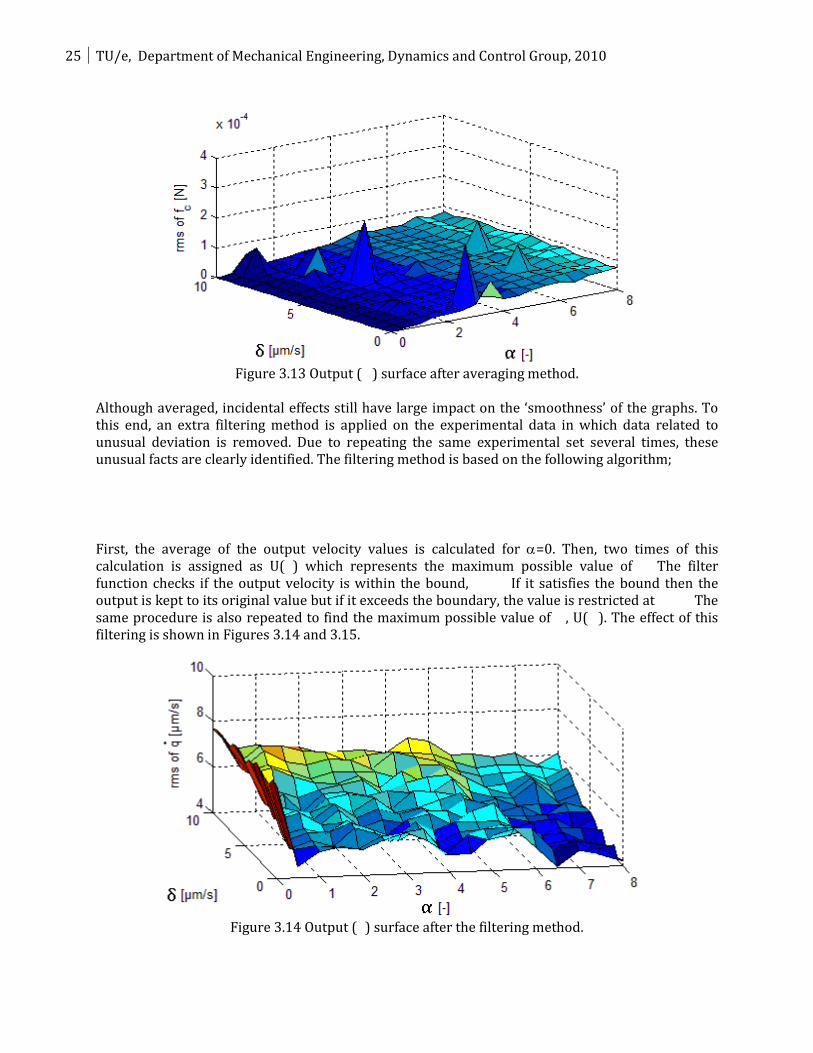
3.2.3 Two-parameters effect

When the experiments in studying the two-parameter (α, δ) effect are performed one by one, it is realized that the output is corrupted by internal and external disturbances. See for example Figure 3.11 which is the result of repeating the same experiment 18 times with fixed value of α=3 and varying δ.

Figure 3.11 Rms of outputs of demonstrating the variety encountered in the experiments by repeating each experiment 18 times under similar conditions.

To reduce the effects of external disturbances, the averaged experimental data is considered to be the main output. This data is used for the graphical analysis as shown in Figures 3.12 and 3.13.

Figure 3.12 Output ( ) surface after averaging method.


Figure 3.13 Output ( ) surface after averaging method.

Although averaged, incidental effects still have large impact on the ‘smoothness’ of the graphs. To this end, an extra filtering method is applied on the experimental data in which data related to unusual deviation is removed. Due to repeating the same experimental set several times, these unusual facts are clearly identified. The filtering method is based on the following algorithm;

First, the average of the output velocity values is calculated for α=0. Then, two times of this calculation is assigned as U( ) which represents the maximum possible value of The filter function checks if the output velocity is within the bound, If it satisfies the bound then the output is kept to its original value but if it exceeds the boundary, the value is restricted at The same procedure is also repeated to find the maximum possible value of , U( ). The effect of this filtering is shown in Figures 3.14 and 3.15.

Figure 3.14 Output ( ) surface after the filtering method.


Figure 3.15 Output ( ) surface after the filtering method.

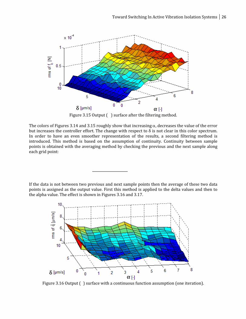
The colors of Figures 3.14 and 3.15 roughly show that increasing α, decreases the value of the error but increases the controller effort. The change with respect to δ is not clear in this color spectrum. In order to have an even smoother representation of the results, a second filtering method is introduced. This method is based on the assumption of continuity. Continuity between sample points is obtained with the averaging method by checking the previous and the next sample along each grid point:

If the data is not between two previous and next sample points then the average of these two data points is assigned as the output value. First this method is applied to the delta values and then to the alpha value. The effect is shown in Figures 3.16 and 3.17.

Figure 3.16 Output ( ) surface with a continuous function assumption (one iteration).


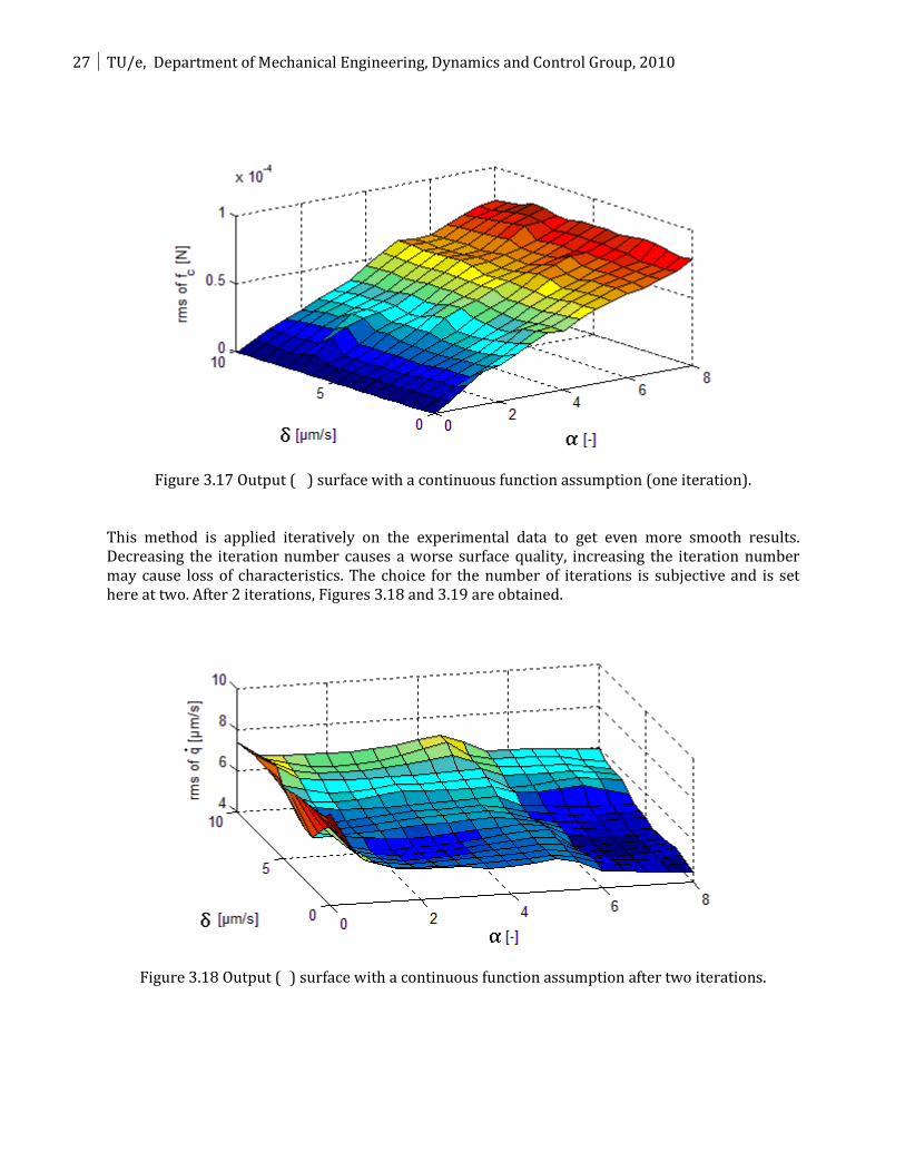
Figure 3.17 Output ( ) surface with a continuous function assumption (one iteration).

This method is applied iteratively on the experimental data to get even more smooth results. Decreasing the iteration number causes a worse surface quality, increasing the iteration number may cause loss of characteristics. The choice for the number of iterations is subjective and is set here at two. After 2 iterations, Figures 3.18 and 3.19 are obtained.

Figure 3.18 Output ( ) surface with a continuous function assumption after two iterations.


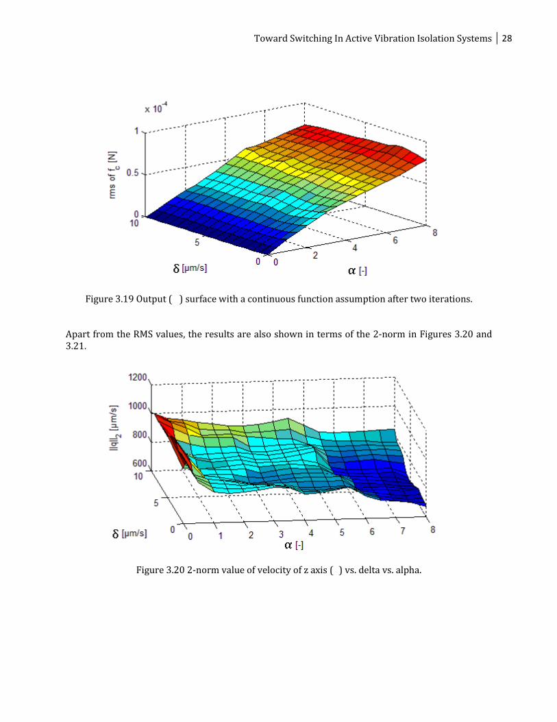
Figure 3.19 Output ( ) surface with a continuous function assumption after two iterations.

Apart from the RMS values, the results are also shown in terms of the 2-norm in Figures 3.20 and 3.21.

Figure 3.20 2-norm value of velocity of z axis ( ) vs. delta vs. alpha.


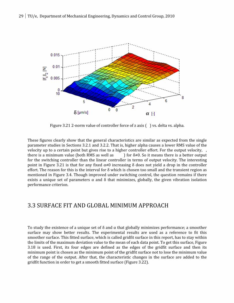
Figure 3.21 2-norm value of controller force of z axis ( ) vs. delta vs. alpha.

These figures clearly show that the general characteristics are similar as expected from the single parameter studies in Sections 3.2.1 and 3.2.2. That is, higher alpha causes a lower RMS value of the velocity up to a certain point but gives rise to a higher controller effort. For the output velocity, , there is a minimum value (both RMS as well as ) for δ≠0. So it means there is a better output for the switching controller than the linear controller in terms of output velocity. The interesting point in Figure 3.21 is that for any fixed α≠0 increasing δ does not yield a drop in the controller effort. The reason for this is the interval for δ which is chosen too small and the transient region as mentioned in Figure 3.4. Though improved under switching control, the question remains if there exists a unique set of parameters α and δ that minimizes, globally, the given vibration isolation performance criterion.

3.3 SURFACE FIT AND GLOBAL MINIMUM APPROACH

To study the existence of a unique set of δ and α that globally minimizes performance; a smoother surface may show better results. The experimental results are used as a reference to fit this smoother surface. This fitted surface, which is called gridfit surface in this report, has to stay within the limits of the maximum deviation value to the mean of each data point. To get this surface, Figure 3.18 is used. First, its four edges are defined as the edges of the gridfit surface and then its minimum point is chosen as the minimum point of the gridfit surface not to lose the minimum value of the range of the output. After that, the characteristic changes in the surface are added to the gridfit function in order to get a smooth fitted surface (Figure 3.22).


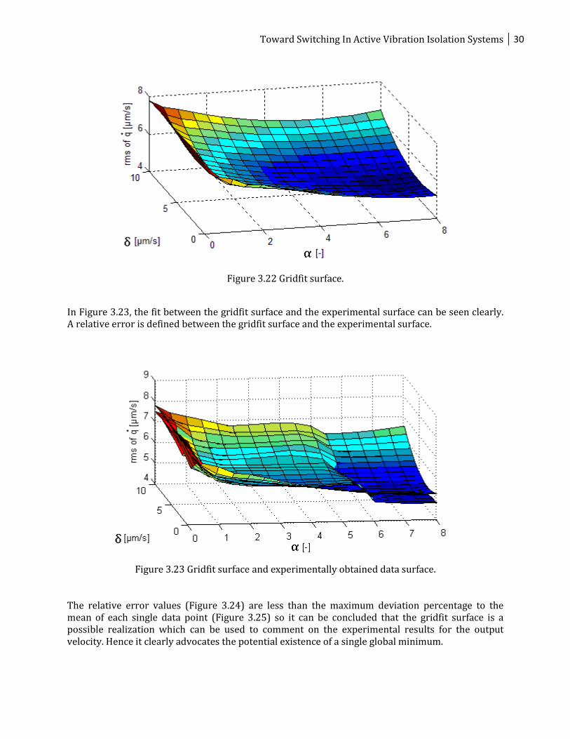
Figure 3.22 Gridfit surface.

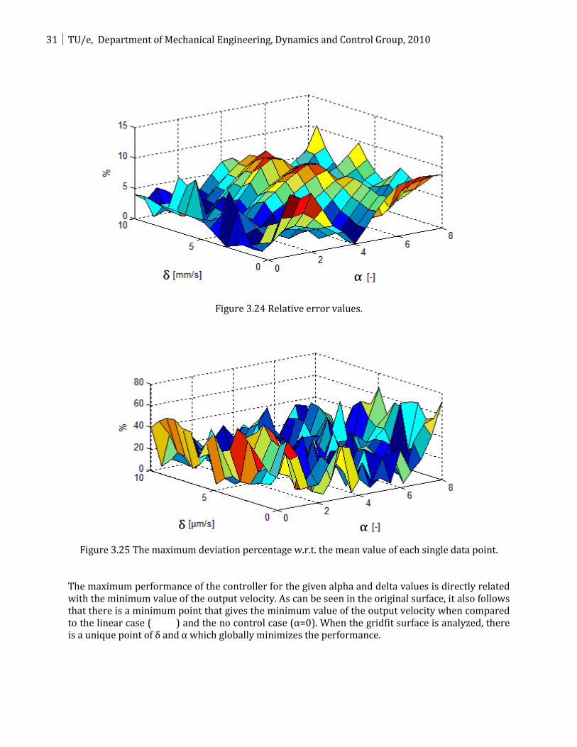
In Figure 3.23, the fit between the gridfit surface and the experimental surface can be seen clearly. A relative error is defined between the gridfit surface and the experimental surface.

Figure 3.23 Gridfit surface and experimentally obtained data surface.

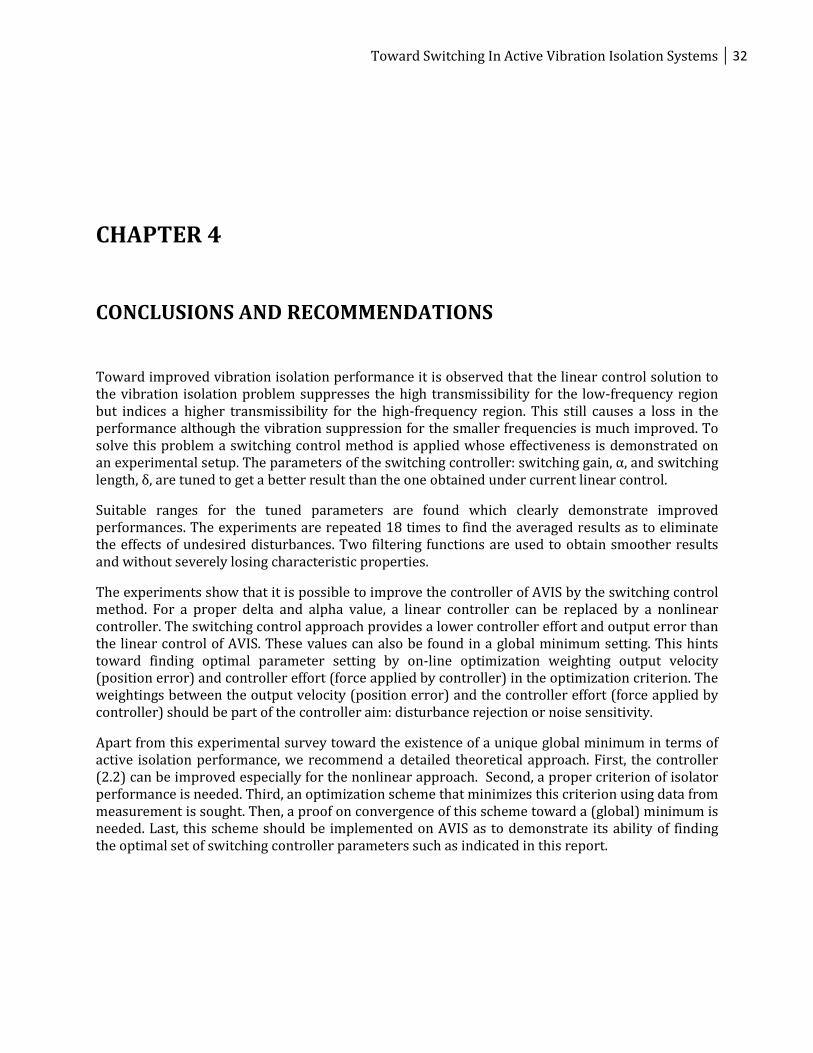
The relative error values (Figure 3.24) are less than the maximum deviation percentage to the mean of each single data point (Figure 3.25) so it can be concluded that the gridfit surface is a possible realization which can be used to comment on the experimental results for the output velocity. Hence it clearly advocates the potential existence of a single global minimum.


Figure 3.24 Relative error values.

Figure 3.25 The maximum deviation percentage w.r.t. the mean value of each single data point.

The maximum performance of the controller for the given alpha and delta values is directly related with the minimum value of the output velocity. As can be seen in the original surface, it also follows that there is a minimum point that gives the minimum value of the output velocity when compared to the linear case ( ) and the no control case (α=0). When the gridfit surface is analyzed, there is a unique point of δ and α which globally minimizes the performance.


CHAPTER 4

CONCLUSIONS AND RECOMMENDATIONS

Toward improved vibration isolation performance it is observed that the linear control solution to the vibration isolation problem suppresses the high transmissibility for the low-frequency region but indices a higher transmissibility for the high-frequency region. This still causes a loss in the performance although the vibration suppression for the smaller frequencies is much improved. To solve this problem a switching control method is applied whose effectiveness is demonstrated on an experimental setup. The parameters of the switching controller: switching gain, α, and switching length, δ, are tuned to get a better result than the one obtained under current linear control.

Suitable ranges for the tuned parameters are found which clearly demonstrate improved performances. The experiments are repeated 18 times to find the averaged results as to eliminate the effects of undesired disturbances. Two filtering functions are used to obtain smoother results and without severely losing characteristic properties.

The experiments show that it is possible to improve the controller of AVIS by the switching control method. For a proper delta and alpha value, a linear controller can be replaced by a nonlinear controller. The switching control approach provides a lower controller effort and output error than the linear control of AVIS. These values can also be found in a global minimum setting. This hints toward finding optimal parameter setting by on-line optimization weighting output velocity (position error) and controller effort (force applied by controller) in the optimization criterion. The weightings between the output velocity (position error) and the controller effort (force applied by controller) should be part of the controller aim: disturbance rejection or noise sensitivity.

Apart from this experimental survey toward the existence of a unique global minimum in terms of active isolation performance, we recommend a detailed theoretical approach. First, the controller (2.2) can be improved especially for the nonlinear approach. Second, a proper criterion of isolator performance is needed. Third, an optimization scheme that minimizes this criterion using data from measurement is sought. Then, a proof on convergence of this scheme toward a (global) minimum is needed. Last, this scheme should be implemented on AVIS as to demonstrate its ability of finding the optimal set of switching controller parameters such as indicated in this report.



Bibliography

[1] N.G.M. Rademakers, Modelling, Identification and Multivariable Control of an Active Vibration Isolation System. Master’s Thesis. Report No. DCT 2005.63 [2] N.G.M. Rademakers, AVIS Manual, Eindhoven University of Technology Department of Mechanical Engineering Dynamics and Control Group Eindhoven, June 21, 2005 [3] MF Heertjes, N van de Wouw, and WPMH Heemels. Switching Control in Active Vibration Isolation, ENOC 2008, Saint Petersburg, Russia. [4] D. Sciulli, Dynamics and Control for Vibration Isolation Design, Virginia Polytechnic Institute, April, 1997 [5] John J. Kim, Barry Controls Brighton, MA Hal Amick, Colin Gordon & Associates San Mateo, CA, Active Vibration Control in Fabs, Reprinted from Semiconductor International, July, 1997 [6] MF Heertjes, BPT van Goch, and H Nijmeijer, Optimal Switching Control of Motion Stages, submitted to IFAC Mechatronics 2010, Cambridge, Massachusetts, USA. [7] ZC Chen, INTRODUCTION TO SCANNING TUNNELING MICROSCOPY, Chapter 10 Vibration isolation 237-250, 1990. [8] P.A.R. de Schrijver, Experimental modal analysis of the tyre measurement tower, DCT 2005.112. [9] R.J.E. Merry, Experimental modal analysis of the H-drive, DCT 2003.78.