Download ppt - The Demand for Goods Chapter-5. In This Chapter…. 5.1.Why is demand curve downward slopping? 5.2. How to measure behavioral responses of consumers to

The Demand for Goods

Chapter-5

In This Chapter….

5.1. Why is demand curve downward slopping?

5.2. How to measure behavioral responses of consumers to changes in determinants of demand (Elasticity)?

5.3. The Effect of Elasticity on the Revenue of the Producer (Seller).

5.3. How Consumers Allocate their Income Among Competing Ends?

5.1. What Explains the Consumer Behavior?

What determines what we buy? How we buy?

What leads us to buy some goods while rejecting others?

Why do we buy more at lower prices and less at higher prices?

5.1.What Explains the Consumer Behavior?

Two Explanations

The Sociopsychiatric Explanation The Economic Explanation

5.1.What Explains the Consumer Behavior?

1. The Sociopsychiatric Explanation

In Freud’s view, higher levels of consumption satisfy our basic drives for security, sex, and ego gratification.

According to sociologists, consuming more is an expression of identity that provokes recognition or social acceptance.

5.1. What Explains the Consumer Behavior?

The Economic Explanation

In explaining consumer behavior, economists focus on the demand for goods and services.

Demand is the willingness and ability to buy specific quantities of a good at alternative prices in a given time period, ceteris paribus.


An individual’s demand for a product is determined by:

– Tastes—desire for this and other goods.– Income—of the consumer.– Expectations—for income, prices, tastes.– Other goods—their availability and prices.


Economists use the Demand Curve to Explain the consumer behavior… how consumer tastes affect consumption decisions. Law of demand: Ceteris paribus, individuals buy

less quantities, when prices are higher and more quantities when prices are lower.

They do so because they have a goal of getting maximum Possible Satisfaction (Pleasure) from their limited resources.

Utility

The Economic Explanation Utility is the pleasure or satisfaction

obtained from a good or service. Utility Theory

Measuring Utility (Satisfaction) Cardinal Units (absolute numbers

indicating levels): Utils

Ordinal Unity (Rankings, Orders of preferences)


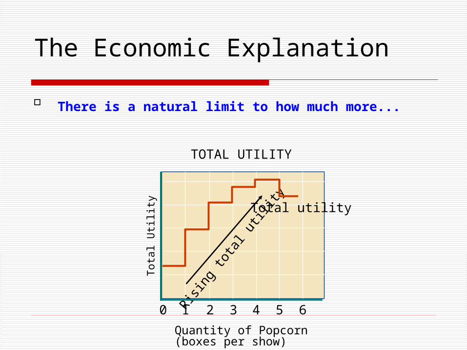
Total Utility is the amount of satisfaction obtained from entire consumption of a product.

The more we consume of a product the more utility (satisfaction) we obtain. I.e., More is Preferred to Less!

Thus the more pleasure (utility) a product gives us, the higher the price we’re willing to pay for it.


However, more is not always and necessarily better.

Two Distinct Levels of Satisfaction:1. Total Utility2. Marginal (additional) Utility


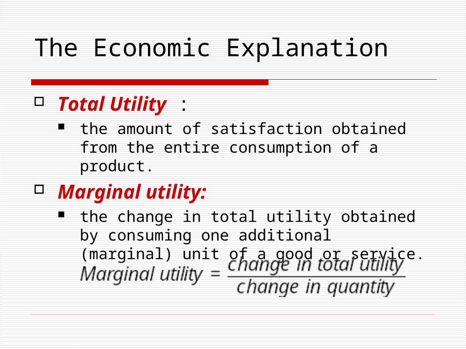
Total Utility : the amount of satisfaction obtained from the

entire consumption of a product. Marginal utility:

the change in total utility obtained by consuming one additional (marginal) unit of a good or service.


There is a natural limit to how much more...

Tot

al U

tility

10 2 3 4 5 6

Quantity of Popcorn(boxes per show)

Total utilityRisi

ng to

tal u

tility

TOTAL UTILITY


Although we prefer more to less, more is not always and necessary better …

Human Behavior: When we have more and more of some thing we start

to value it less and less. We do so… The additional satisfaction we get from consuming

one more unit of the same product is lower than the level of satisfaction we obtain from consuming earlier units of the product.

Declining Marginal Utility

The Economic ExplanationT

otal

Util

ity

10 2 3 4 5 6


Total utility

Rising

tota

l utili

ty

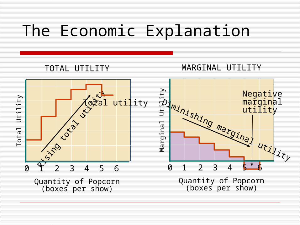
TOTAL UTILITY

Mar

gina

l Util

ity10 2 3 4


Diminishing marginal utility

5 6

Negative marginal utility

MARGINAL UTILITY

Diminishing Marginal Utility

According to the law of diminishing marginal utility, the marginal utility of a good declines as more of it is consumed in a given time period.

As long as marginal utility is positive, total utility must be increasing.

Diminishing Marginal Utility

According to the law of diminishing utility, each successive unit of a good consumed yields less additional utility.

Eventually, additional quantities of a good yield increasingly smaller increments of satisfaction. Downward slopping Demand Curve


Implication… Our consumption decision is guided by

not by how much total satisfaction we get, but by how much additional satisfaction we get when consuming one more unit of a product

The Economic ExplanationDemand Curve: Price and Quantity relationship (Why is it downward slopping?)

Tastes, through marginal utility, tells us how much we desire particular goods.

Price tell us how much of a good we will buy.

The more marginal utility a product delivers, the more a consumer is willing to pay, ceteris paribus.

As the marginal utility of a good diminishes, so does our willingness to pay.

5.2. Gagging Responses to Changes in the Determinants of Demand


According to the law of demand, the quantity of a good demanded in a given time period increases as its price falls, ceteris paribus.

(Own Price, Income, Price of other Products,….)


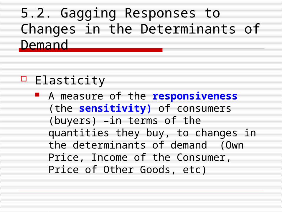
Elasticity A measure of the responsiveness (the

sensitivity) of consumers (buyers) –in terms of the quantities they buy, to changes in the determinants of demand (Own Price, Income of the Consumer, Price of Other Goods, etc)


Elasticity Price Elasticity of Demand Income Elasticity of Demand Cross Price Elasticity of Demand

Price Elasticity (E)

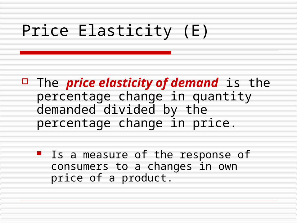
The price elasticity of demand is the percentage change in quantity demanded divided by the percentage change in price.

Is a measure of the response of consumers to a changes in own price of a product.

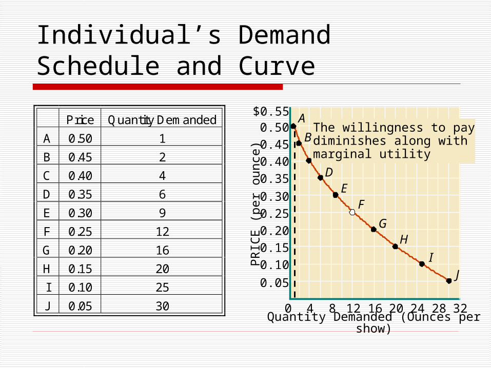
Individual’s Demand Schedule and Curve

Quantity Demanded (Ounces per show)

PR

ICE

(pe

r ou

nce)

A

B

CD

EF

GH

IJ

0 4 8 12 16 20 24 28 32

0.05

0.10

0.150.20

0.250.30

0.35

0.400.450.50

$0.55Price Quantity Demanded

A 0.50 1

B 0.45 2

C 0.40 4

D 0.35 6

E 0.30 9

F 0.25 12

G 0.20 16

H 0.15 20

I 0.10 25

J 0.05 30

The willingness to paydiminishes along withmarginal utility

Computing Price Elasticity (E)

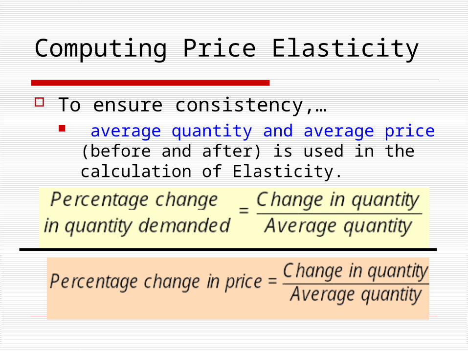
Computing Price Elasticity

To ensure consistency,… average quantity and average price

(before and after) is used in the calculation of Elasticity.

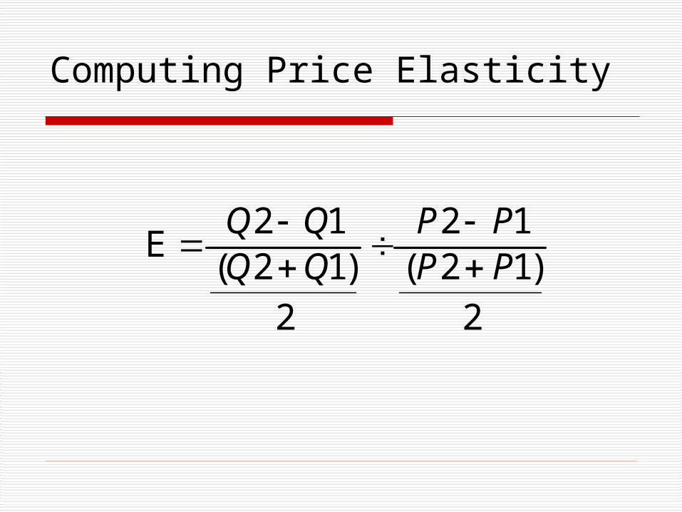
Computing Price Elasticity

2

1212

2

1212

)()(E

PPPP

QQQQ

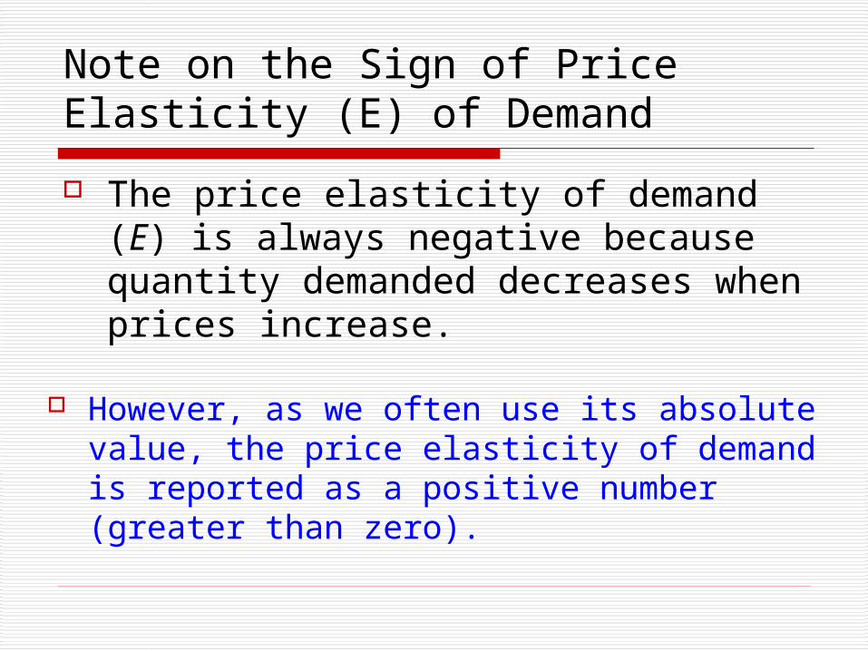
Note on the Sign of Price Elasticity (E) of Demand

The price elasticity of demand (E) is always negative because quantity demanded decreases when prices increase.

However, as we often use its absolute value, the price elasticity of demand is reported as a positive number (greater than zero).

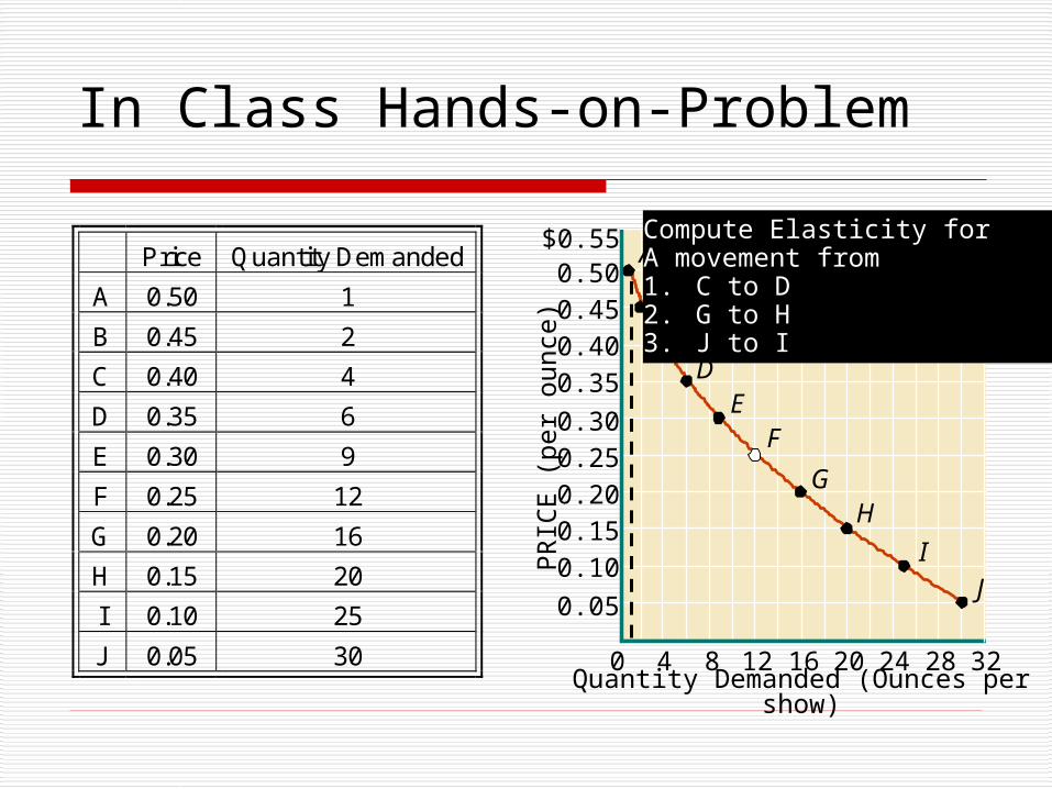
In Class Hands-on-Problem

Quantity Demanded (Ounces per show)

PR

ICE

(pe

r ou

nce)

A

B

CD

EF

GH

IJ

0 4 8 12 16 20 24 28 32

0.05

0.10

0.150.20

0.250.30

0.35

0.400.450.50

$0.55Price Quantity Demanded

A 0.50 1

B 0.45 2

C 0.40 4

D 0.35 6

E 0.30 9

F 0.25 12

G 0.20 16

H 0.15 20

I 0.10 25

J 0.05 30

Compute Elasticity for A movement from 1. C to D2. G to H3. J to I

Possible Values of Elasticity: |E|

E can take any value between from 0 to infinity

Five Broad categories

0<E<1; E=1; 1<E<Positive Infinity Two extreme Values (E=0 ; E=Positive

Infinity)

Elastic, Inelastic, Unitary Elastic Demand

If E is larger than 1, demand is elastic. Consumer response is large relative to the change

in price. Relatively Flat Demand Curve

If E equals 1, demand is unitary elastic.

If E is less than 1, demand is inelastic. Consumers aren’t very responsive to price

changes. Relatively Steeper Demand Curve

Elasticity Estimates

Elastic Unitary Inelastic Price

Elasticity Estimate

Price Elasticity Estimate

Price Elasticity Estimate

Airline travel (long run)

2.4 Private education

1.1 Cigarettes 0.4

Restaurant meals

2.3 Radios and television

1.2 Coffee 0.3

Fresh fish 2.2 Shoes 0.9 Gasoline (short run)

0.2

New cars (short run)

1.2-1.5 Movies 0.9 Electricity (in homes)

0.1

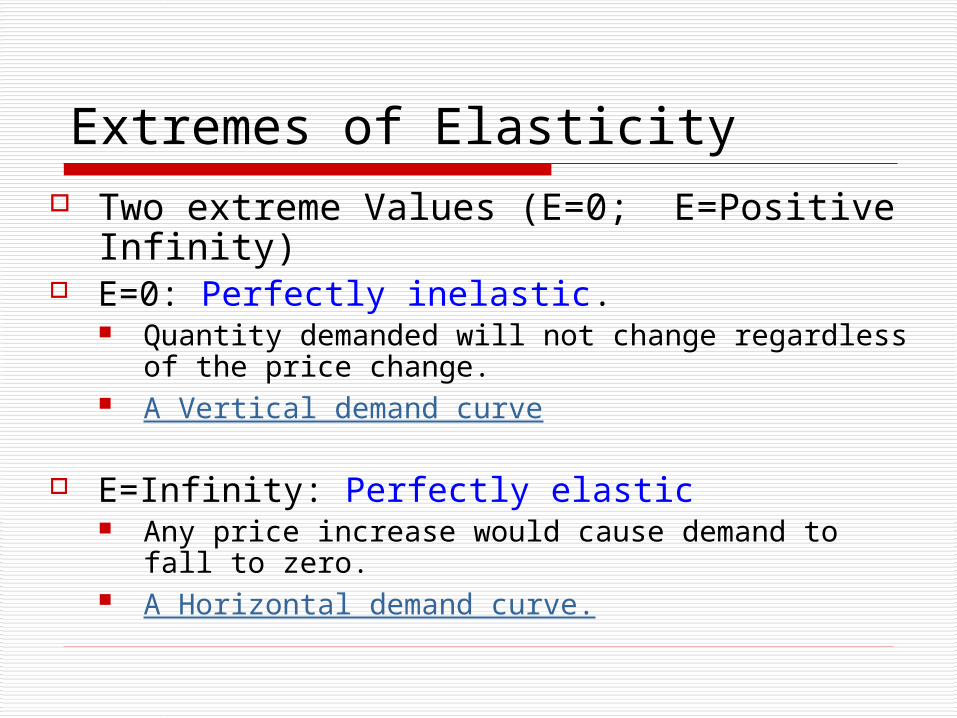
Extremes of Elasticity Two extreme Values (E=0; E=Positive

Infinity) E=0: Perfectly inelastic.

Quantity demanded will not change regardless of the price change.

A Vertical demand curve

E=Infinity: Perfectly elastic Any price increase would cause demand to fall to

zero. A Horizontal demand curve.

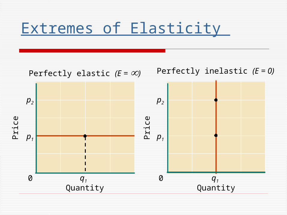
Extremes of Elasticity

p1

p2

q10Quantity

Pri

ce

Perfectly elastic (E = )

p1

p2

q10Quantity

Pri

ce

Perfectly inelastic (E = 0)

Determinants of Elasticity

The price elasticity of demand is influenced by all of the determinants of demand.

Four factors are particularly worth noting: Necessities vs. Luxuries. Availability of Substitutes. Relative Price (to income). Time.

Necessities vs. Luxuries

Necessities are goods that are critical to our day-to-day life. Demand for necessities is relatively

inelastic• Luxuries are goods we would like to

have but are not likely to buy unless our income jumps or the price declines sharply. Demand for luxury goods is relatively

elastic.

Availability of Substitutes

If a good has relatively many substitutes, consumers are highly sensitive to changes in the price of the good.

Thus the greater the availability of substitutes, the higher is the price elasticity of demand…relatively elastic

Relative Price (to income)

Consumers are more sensitive to changes in prices of goods that account for a relatively larger share of their budget (at higher price level) than those that account for relatively smaller share of their budget (lower price)

The higher the price of a good relative to a

consumer’s income, the higher the elasticity of demand.

The price elasticity of demand declines as price moves down the demand curve.

Time

Consumers are better able to change their buying habits over the long-run (thus more sensitive to changes in prices) than in the short-run (Less sensitive).

Thus in the long-run price elasticity of demand is higher than the short-run elasticity.

Elasticities and the Other Determinants of Demand

Price Elasticity of Demand

Income Elasticity of Demand Cross Price Elasticity of Demand

Shifts vs. Movements

Recall: When the price changes, the outcome is a

movement along the same demand curve.

When any one of the underlying determinants of demand (other than own price of the good) changes, the entire demand curve shifts.

Income and prices of other goods are among such factors

Income Elasticity

An increase (decrease) in consumer income will cause a rightward (leftward) shift in demand.

I.e., consumers will purchase more at any price than they did prior to the increase in income.

Income Elasticity

Quantity of Popcorn (ounces per show)

Price

of P

opco

rn (d

olla

rs p

er o

unce

)

Shift

D2 (after income rise)

D1 (before income rise)

NF

0 12 16

0.25

Income Elasticity

Income elasticity of demand is the measure of the percentage change in quantity demanded by the consumer resulting from a percent change in income of the consumer.

Computing Income Elasticity

As with price elasticity, income elasticity is computed using average values for the changes in quantity and income.

Normal vs. Inferior Goods

A normal good has an income elasticity of demand greater than zero. A normal good is a good for which

demand rises when income rises. An inferior good has an income

elasticity of demand less than zero. An inferior good is a good for which

demand decreases when income rises.

Cross-Price Elasticity

A change in the price of one good affects the demand for another.

The decision to buy a good also depends on the prices of substitutes and complements of that good.

Cross-Price Elasticity

Substitute goods are goods that substitute for each other. When the price of good X rises, the demand for

good Y increases, ceteris paribus.

Complementary goods are goods frequently consumed in combination. When the price of good X rises, the demand for

complementary good Y falls, ceteris paribus.

Substitutes and Complements

R FD3

D1

D2

0 8 12

0.25

Quantity of Popcorn (ounces per show)

Pri

ce o

f Pop

corn

(cen

ts p

er

ou

nce

)

Calculating Cross-Price Elasticity Cross price elasticity is the

percentage change in the quantity demanded of X divided by percentage change in price of Y.

Sign of Cross-Price Elasticity

When the cross-price elasticity of demand has a negative sign the two goods are complementary goods.

When the cross-price elasticity of demand has a positive sign the two goods are substitute goods.

Elasticity and Revenue (Elasticity and Pricing Decision)

5.3. Elasticity and Pricing Decision

Strong relationship between price elasticity and total revenue.

Total revenue is The price of a product multiplied by the quantity sold in a given time period.

Total revenue = Price X Quantity sold TR= P X Q


TR = P x Q Given the law of demand ( Price and

Quantity are inversely related), what happens to the total revenue of the seller when there is:

1. A Price Hike?2. A Price Decline (Sales Discount)?

5.3. Elasticity and Pricing Decision A price hike increases total revenue of

a seller only if demand is inelastic (E < 1). if demand is elastic (E > 1), a hike in

price reduces total revenue of the seller.

if demand is unitary elastic (E = 1), hike in price does not change total revenue of the seller


A decline in price (Sales Discount) on the other hand increases total revenue of a seller if the demand is elastic (E > 1).

If the demand is inelastic (E<1) sales discount doesn’t increase the total revenue of the producer

Implication?

Implication?

1. Most of the time, we get discounts for luxury goods than necessities; and on goods that account for relatively larger share of our budget (those that have higher prices)

2. The impact of a price change on total revenue of the seller depends on the price elasticity of demand.

3. Price elasticity changes along a demand curve.

Price Elasticity and Total Revenue

Price Elasticity and Total Revenue

2 4 6 10 12 14 16 18 20 22 24 26 28 30 3280

$0.550.500.450.400.350.300.250.200.150.100.05

QUANTITY DEMANDED (ounces per show)

PR

ICE

(pe

r ou

nce

) BC

At higher prices E > 1

At Lower prices E < 1

$876543210

PR

ICE

10 20 30 40 50 60 70 80 90 100 110

Elastic E > 1

Unit elastic E = 1

Inelastic E < 1

The demand curve

$225200175150125100755025

0

Elastic E > 1

Inelastic E < 1

10 20 30 40 50 60 70 80 90 100 110

TO

TA

L R

EV

EN

UE

Total revenueE = 1

How consumers Decide to Allocate their Income

(Choosing Among Products)

5.4. Choosing Among Products

Goal: Utility Maximization Consumers should choose the optimal

consumption combination.

the mix of consumer purchases that maximizes the utility attainable from available income (budget).


The purchase of any one single good also means giving up the opportunity to buy more of other goods.

Recall Opportunity costs – The alternatively most desired goods or

services that are forgone in order to obtain something else.


Economist assume that consumers have Rational Behavior.

Rational behavior requires one to compare the anticipated utility of each expenditure with its cost.

Thus to maximize utility, the consumer should choose that good which delivers the most marginal utility per dollar.

Example…

Utility Maximizing Rule

If a person could get more utility per dollar by buying good X, then she should continue to buy good X.


If a person could get more utility per dollar by buying good Y, then she should continue to buy good Y.


Continue this process until the ratios are equal – only then will utility be maximized.

Example…

The consumer has $10; Px=$1 and Py=$2. To get Max Utility How much of each good should the consumer purchase?

The Outcome: Optimal

Economic theory predicts that the final choices of consumers -- the equilibrium outcome -- will be optimal.

There is no better combination that gives more utility for the money (budget), given the prices


Why advertising then?


Some advertising is intended to provide information about new or existing products.

A great deal more of advertising is designed to exploit our senses and lack of knowledge. Advertising can’t be blamed for our

foolish consumption


A successful advertising campaign is one that shifts the demand curve to the right.

Impact of Advertising on the Demand Curve

Quantity Demanded (units per time period)0

Pric

e (d

olla

rs p

er u

nit) Demand curve

after advertising

Demand curve before advertising

P

Q1 Q2