q 2000 RAS
The evolution of bodies orbiting in the trans-Neptunian region on tointermediate-type orbits
M. D. Maran and I. P. Williamsw
Astronomy Unit, Queen Mary and Westfield College, Mile End Road, London E1 4NS
Accepted 2000 June 5. Received 2000 June 5; in original form 2000 February 11
A B S T R A C T
We investigate the dynamical evolution of 210 hypothetical massless bodies initially situated
between 10 and 30 au from the Sun in order to determine the general characteristics of
the evolved system. This is of particular relevance to the understanding of the origin of
Edgeworth±Kuiper belt objects on scattered intermediate orbits, such as 1996TL66, which
have high eccentricity and semimajor axis but nevertheless have perihelion in the region
between 30 and 50 au from the Sun.
Key words: celestial mechanics, stellar dynamics ± minor planets, asteroids ± planets and
satellites: general.
1 I N T R O D U C T I O N
Historically, our knowledge of the structure and dynamics of the
Solar system beyond the orbit of Neptune had been based on a
combination of theoretical modelling and deductions from the
observational data regarding very long period or new comets
entering the inner Solar system. One obvious consequence of such
studies was the recognition that a reservoir of comets at very large
heliocentric distances was necessary in order to account for the
current influx rate. The best known and most widely accepted
form for this reservoir is the Oort cloud, named after the
hypothesis by Oort (1950) that a spherical cloud of cometary
nuclei, consisting of some 1011 bodies with semimajor axis
between 104 and 105 au existed. Various authors subsequently
added families of subclouds within the same general framework.
Somewhat earlier than Oort, Edgeworth (1943) had postulated
that a ring of bodies, lying roughly in the ecliptic and located
just beyond the Neptunian orbit existed and could be the source
of comets. A very similar scenario was subsequently, but
independently, described by Kuiper (1951).
By the late 1980s, numerical studies such as those by Duncan,
Quinn & Tremaine (1988), Stagg & Bailey (1989) and Quinn,
Tremaine & Duncan (1990) had shown that the influx of short-
period comets required the existence of some belt such as the
Edgeworth±Kuiper Belt. It was thus very exciting, but not
surprising, that Jewitt & Luu (1992) found the first potential
member of this belt, 1992QB1. The first surprise came when it was
recognized than 1993SC (Williams et al. 1995) moved on an orbit
that was very close to the location of the 2:3 mean motion
resonance with Neptune, i.e. the same type of orbit that Pluto
moves on. At the time of writing (1999 December), about 200
bodies have been discovered in the region, 32 of which are close
to the 2:3 resonance with Neptune and most of the remainder of
which are in the traditional Edgeworth±Kuiper belt. Those in
the first group move on orbits with a semimajor axis very close
to 39.5 au, while the remainder with a few exceptions have a
semimajor axis between 41 and 46 au. Leaving aside 1996TL66,
which will be discussed in more detail later, the largest semimajor
axis at present is for 1997SZ10 at 48.7 au, and this object also has
the largest aphelion distance at 66.9 au. In terms of coplanarity, 85
of the objects have an inclination less than 108, while 57 have an
inclination less than 58. The highest recorded inclination so far is
408 for 1999CY118.
As already mentioned, the first major exception to the above
picture discovered was 1996TL66 (Luu et al. 1997). The currently
published values of the orbital parameters give a semimajor axis
of 85.754 au and an aphelion distance of 137 au, implying an
eccentricity of 0.594. Its inclination is also towards the high end of
the spectrum at 238: 9. It is no longer unique, with others on similar
orbits having since been discovered (see Trujillo, Jewitt & Luu
2000 for a comparison of current orbits). However, we shall use
1996TL66 as a typical body on this type of scattered orbit. We
should also remember that a further class of objects, namely the
Centaurs, were discovered within the last 20 yr, and that these
occupy roughly the same region of space as the giant planets,
Saturn through to Neptune. It is also generally recognized that this
region is chaotic on a time-scale comparable to the age of the
Solar system.
The origin of the trans-Neptunian objects has been a topic of
some debate (see for example Stern 1996; Kenyon & Luu 1998).
We do not wish to contribute to the full debate regarding the
origin, the choices being formation in approximately the location
that they are currently found in, formation in the Oort cloud with a
subsequent orbital evolution to their present location or formation
closer in, perhaps in the Uranus±Neptune region, with subsequent
ejection. We should note that the second alternative begs the
Mon. Not. R. Astron. Soc. 318, 482±492 (2000)
w E-mail: [email protected]
question of how the Oort cloud formed. In this paper we
investigate a simpler problem than that of the origin of all of the
outer Solar system. We enquire where objects initially located in
this region occupied by the giant planets, i.e. roughly between
Saturn and Neptune, will tend to evolve to, and in particular,
whether orbits similar to that of 1996TL66 will be generated. As a
secondary aim, some knowledge of the other types of orbits that
we might expect from this process will also become evident. It
should also be noted that as we have no dissipative forces present,
all the equations of motion are time reversible, so that in principle
(although not on the same time-scale) the final orbits can evolve to
the initial orbits. We do this with the aid of a computer model by
integrating numerically the equations of motion of test bodies
initially moving in the relevant region of space and analysing the
subsequent evolution.
2 T H E M O D E L U S E D
Massless test particles were generated with semimajor axis
uniformly distributed within the region of interest, that is between
10 and 30 au. Steps of 1 au were used, because we believed that
this would give adequate spatial coverage of the location. This
requires 21 different values of the semimajor axis. For each value
of the semimajor axis, eccentricities were uniformly distributed
between 0 and 0.9 in steps of 0.1. This generates a set of 210 test
particles. The inclinations were initially assumed to be zero,
because any non-zero inclination also requires both the longitude
of the ascending node and the argument of perihelion to be
specified. Doing this thus represents a major increase in the
number of free parameters and consequently in the number of test
particles required to fill the phase-space, a major consideration
because long-term integrations are to be performed. Within
the context of formation in a Solar nebula, the assumption of
coplanarity is not very unrealistic, and, because the major planets
are not strictly coplanar, there will be evolution in inclination so
that the values do not stay zero very long. The Solar system is
assumed to consist of the planets Jupiter, Saturn, Uranus and
Neptune, with the mass of the inner planets being added to that of
the Sun. Pluto was not included because of its small mass. All
bodies are regarded as point masses.
The equations of motion of the 210 test particles were
numerically integrated using the Runge±Kutta±Nystrom integra-
tor described by Dormand, El-Mikkai & Prince (1987), with
the coefficients transmitted electronically by Dormand, thus
minimizing the possibility of copy-errors entering through these
coefficients. The dominant factor limiting the length of time over
which numerical integrations can be performed, or in reality the
total number of time-steps, as was discussed by Roy et al. (1988),
is rounding error, that is the accuracy with which any numerical
value can be stored or manipulated and the way in which such
errors propagate through the integrations as they progress. They
showed that for the outer Solar system with an integrator of the
type we are using and double precision information storage, the
limit on the length of integration before the propagated rounding
error starts to dominate and in effect produce random fluctuations
is about 108 yr. We thus restrict our integrations to this time
interval. Our integrations confirm this conclusion regarding the
time-scale, with behaviour becoming erratic as we approach the
limit, but generally not so before then. Hence, for the major part
of the time interval, we believe that, in a statistical sense, the
behaviour of the bodies in our simulation accurately reflects
reality.
3 T H E R E S U LT S
A numerical integration naturally produces only numerical results
and so the actual output from running the integrations described
above is to produce a set of numerical values for the position and
velocity of each test particle after each time-step. As there are
more than 109 time-steps per run, even recording all this data is a
mammoth task. Consequently we have only in general stored the
output at time intervals of 104 yr for each set of values of the
velocity and position of a body. The data can of course be
converted in the usual way to energy per unit mass and angular
momentum per unit mass and these can then be used to give the
five osculating elements of heliocentric orbits and the true
anomaly of the bodies at each of the time-steps.
If presented in numerical form, this is a vast data set and
reproducing these numerical values serves no useful purpose.
Instead, we present the information in diagrammatic format,
showing the evolution of the orbital elements. However, even
doing this for all the orbital elements for all 210 test objects would
still produce 1050 diagrams. Fortunately, we are not interested in
the detailed behaviour of every individual object, but rather in an
overview of the behaviour of the whole family. Consequently we
shall concentrate on a discussion of the typical behaviour pattern
for identifiable subgroups of the whole set. Some of these sub-
groups, and their resulting behaviour, are almost predictable from
the initial orbit and a simplistic understanding of orbital
mechanics. In particular, we might expect bodies with initial
orbits that cross those of either Jupiter or Saturn to have close
encounters with either of these planets early on in the evolution
and so experience large perturbations in their orbits, probably
leading to many cases of loss from the system. For convenience,
we call these bodies of Type 1. Similarly, a number of the test
bodies will have initial orbits that take them close to either or both
of Uranus and Neptune, but not Jupiter or Saturn. They may also
experience significant early perturbations, but these may not be as
severe as for Type 1. We will call these orbits those of Type 2. The
remaining bodies did not start life experiencing large perturba-
tions, although some may evolve into such a state and so have the
possibility of experiencing large perturbations and being lost from
the system. These we will categorize as Type 3 orbits. It should be
noted that these types of orbits have been categorized on the basis
of what common sense dictates to us might happen, not what
actually happened according to the numerical integrations. We
will discuss in turn what actually did take place, but before doing
so we require a working definition of what should be regarded as
`lost from the system', it being impractical to actually integrate
the motion of a body to infinity, or into the Sun. Although it is
possible to follow trends in the semimajor axis or perihelion
distance and make some qualitative judgement based on a
becoming large or q small, doing this avoids the question, for
we then have to define large and small. The simplest measure is to
define a body as lost when its eccentricity becomes unity to some
given level of accuracy. This does not by itself indicate whether
the body is at a large distance or a very small distance, but it does
indicate that the body has effectively been lost from the domain of
interest to us. For practical purposes we chose the value where the
eccentricity is unity to four significant figures. We should add that
even if in a strict sense an individual body that violates this
condition appears not to escape according to the remainder of the
integration, it is almost certain that the integration has now
become very inaccurate and tells us nothing about the subsequent
motion of that particular body. We shall now look at the results of
Orbits in the trans-Neptunian region 483
q 2000 RAS, MNRAS 318, 482±492
the integrations and compare these with the expectations for each
type of motion identified above.
3.1 Type 1
This type consists of the bodies that were moving on initial orbits
that cross the orbits of either or both of Jupiter or Saturn. Because
of the systematic way that we distributed the initial 210 orbits, 104
are Saturn-crossers and of these 52 also cross the orbits of Jupiter.
Note that because the smallest semimajor axis considered was
10 au, there are no bodies within the investigated set that have an
initial orbit that crosses only the orbit of Jupiter. In addition to the
above 104 objects, there are ten objects that are not technically
Saturn-crossers, but have their perihelia so close to Saturn's orbit
that very close encounters are inevitable. For example an orbit
with an initial semimajor axis of 13 au and an eccentricity of 0.2
can approach to within 0.4 au of Saturn. We treat all 114 bodies as
belonging to Type 1. A number of these bodies have initial orbits
that also cross the orbits of Uranus and/or Neptune. As already
mentioned, we might expect bodies on most of these orbits to
evolve in a manner that eventually leads to the loss of the body
from the system, and a number of investigations (e.g. Holman &
Wisdom 1993) have shown that motion in this general region is
chaotic. Hence, it might be argued that as the final results are
fairly predictable, actually carrying out the integrations was a
waste of computer time. Nevertheless, we have carried out the
integrations and there were three main reasons for doing this.
First, the results provide a test of the correctness of our
integrations: if the bodies on these orbits did not in general show
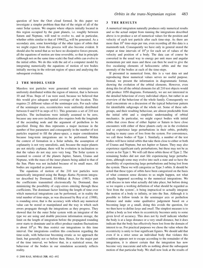
Figure 1. The evolution of the principal orbital elements (a, e and i) of a body on an initial orbit that has close encounters with the major planets and is lost
from the system. This particular body was lost after an interval of only 5 � 105 yr:
484 M. D. Maran and I. P. Williams
q 2000 RAS, MNRAS 318, 482±492
the effects of close encounters with major planets, our model must
be incorrect. Secondly, determining the time-scale over which
bodies are lost is of interest. Thirdly, the evolution of the few
bodies that do not escape from our domain is of considerable
interest because they may be the source of 1996TL66 type objects
and of other real bodies that are found on unusual orbits. The
results of the numerical integrations did confirm the general
expectations: 96 of these bodies were lost within 106 yr and a
further 15 within 107 yr. Thus only 3 survived for the full time-
span of the integration. Rather surprisingly, two of the three
survivors were on orbits that initially crossed both the orbit of
Jupiter and the orbit of Saturn. Both will be discussed later.
Fig. 1 shows the evolution of the principal orbital elements (a, e
and i) of a typical body on an orbit of this first type that was lost
within a time interval of 107 yr. This particular body was initially
on an orbit with a semimajor axis of 20 au and eccentricity of 0.7
and thus was not initially a Jupiter crosser, although it did cross
the orbits of the other three major planets. The initial evolution
must have been fairly rapid, the first plotted point in Fig. 1
showing it with a semimajor axis of 34 au and an eccentricity of
0.72, the perihelion thus being very close to the Saturnian orbit.
Though there are some further changes in the elements over the
next million years, perihelion always remains close to the
Saturnian orbit until it embarks on a disastrous evolution with
eccentricity rapidly approaching unity and the semimajor axis
climbing to at least 100 au. Note that to make a comparison
between the different types of evolution easier, we have plotted all
the figures to the same vertical scales, namely, a between 0 and
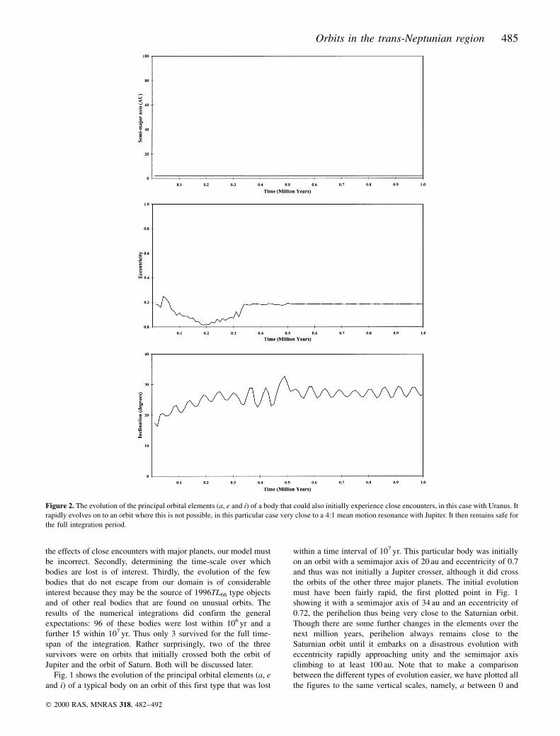
Figure 2. The evolution of the principal orbital elements (a, e and i) of a body that could also initially experience close encounters, in this case with Uranus. It
rapidly evolves on to an orbit where this is not possible, in this particular case very close to a 4:1 mean motion resonance with Jupiter. It then remains safe for
the full integration period.
Orbits in the trans-Neptunian region 485
q 2000 RAS, MNRAS 318, 482±492
100 au, e between 0 and 1 and inclination between 08 and 408.For the next 2 � 106 yr �3 � 106 yr in total), the eccentricity
approaches closer and closer to unity, while the semimajor axis
continues to climb, reaching a value of 6000 au (not visible in the
figure, but deducable from the numerical printout of the results).
At this point it has satisfied our criteria for being lost from
the system. There is little of interest in the behaviour of the
inclination, which climbs to about 108 and then remains roughly at
that value.
Turning to the three objects that survived for 107 yr, one showed
the same characteristics as many of those that were lost. It was on
an initial orbit with semimajor axis of 27 au and an eccentricity of
0.7, implying an initial perihelion distance of 8.1 au, thus it also
was not a Jupiter crosser but with perihelion not far from the
Saturnian orbit. It showed a similar evolution to that described
above, namely an increasing eccentricity, reaching values in
excess of 0.9 within the integration period, while the semimajor
axis is also increasing, reaching 130 au within 1 � 106 yr: This
evolution is so similar to that discussed above that it seems very
likely that it will also be lost from the system in an interval well
below the age of the Solar system.
The remaining two objects both had an initial eccentricity of
0.8; one had a semimajor axis of 11 au and the other 25 au. The
aphelion of the first is thus at 19.8 au, exceedingly close to the
Uranian orbit, while its perihelion is at 2.2 au, well away from any
perturber within our model, remembering that all the inner planets
were included in the Solar mass. It thus also crosses the orbits of
Jupiter and Saturn, initially at a very low inclination, so that close
encounters with these planets are likely. The evolution of the
orbital element for this body is shown in Fig. 2.
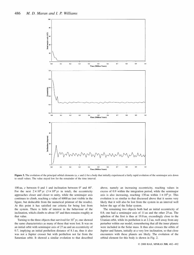
Figure 3. The evolution of the principal orbital elements (a, e and i) for a body that initially experienced a fairly rapid evolution of the semimajor axis down
to small values. The value stayed low for the remainder of the time interval.
486 M. D. Maran and I. P. Williams
q 2000 RAS, MNRAS 318, 482±492
We see that the evolution is fairly uneventful for most of the
time interval, the initial close approaches causing a rapid
evolution on to a very steady orbit with eccentricity around 0.2
and no close approaches to any of the planets included in the
integration. This semimajor axis value is very similar to the initial
perihelion distance. The actual orbit is very similar to that of
asteroid 2, Pallas, although not much weight should be given to
this because of the omission of Earth and Mars from the
integration. It is also close to the 4:1 mean motion resonance
with Jupiter. Despite the initial aphelion being close to Uranus, the
most likely cause of the computed evolution is close encounters
with Jupiter during the early stages.
The initial orbit of the second body crosses the orbits of all four
major perturbers, with a perihelion at 5 au and thus a little inside
the orbit of Jupiter. The evolution of the orbital parameters for this
body is shown as Fig. 3. Again we see a fairly rapid evolution of
the semimajor axis down to around 2 au; it remains at this value
for the remainder of the time interval. The eccentricity and
inclination also reached very similar values, but somewhat more
smoothly than for the first body. These two bodies might represent
the dynamics of a process generally thought to occur in the real
Solar system, namely the conversion of a comet-like orbit to an
asteroid-like orbit. This is consistent with the hypothesis that some
dead comets may be amongst the asteroid population, although
this is totally irrelevant to the main theme of this paper.
3.2 Type 2
This class was defined to consist of bodies that were initially
moving on orbits that cross the orbits of either or both of Uranus
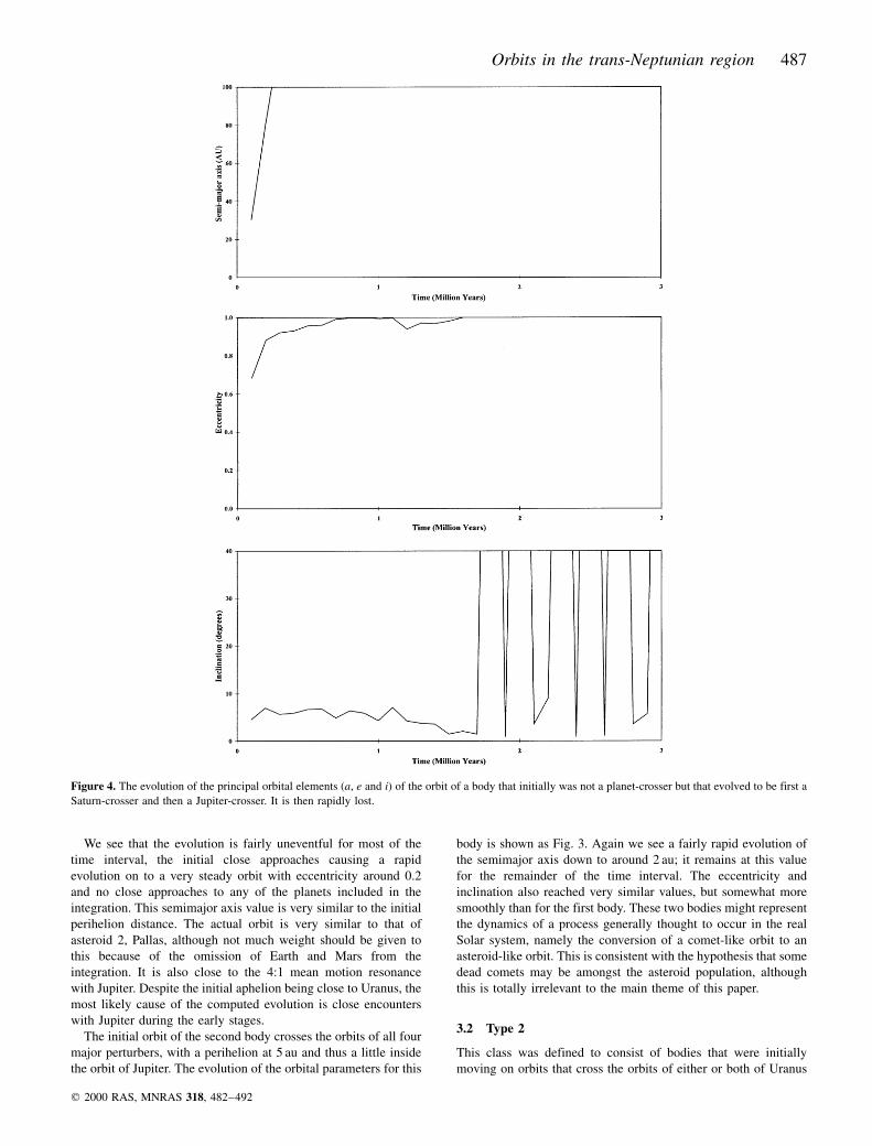
Figure 4. The evolution of the principal orbital elements (a, e and i) of the orbit of a body that initially was not a planet-crosser but that evolved to be first a
Saturn-crosser and then a Jupiter-crosser. It is then rapidly lost.
Orbits in the trans-Neptunian region 487
q 2000 RAS, MNRAS 318, 482±492
or Neptune but not the orbits of either Jupiter or Saturn. Although
an order of magnitude less massive than Jupiter and Saturn,
Uranus and Neptune are nevertheless capable of producing major
perturbations to the orbit of any bodies that get sufficiently close.
Such encounters may cause the body to be lost directly from the
system, or to evolve on to orbits that cross the orbits of either or
both of Jupiter and Saturn, leading to a subsequent evolution
similar to that for bodies belonging to Type 1, or could lead to the
final orbits being very markedly different from the initial orbit but
not lost from the system.
There are 63 bodies that initially moved on orbits belonging to
this type. Of these, 35 were lost from the system within the full
integration interval of 107 yr but, of these, only 11 were lost within
the first million years, indicating that the evolution is slower than
for bodies belonging to Type 1, as one might expect given that the
perturbers are less massive. Figs 4 and 5 show examples of the
evolution of the orbital parameters of two typical bodies belonging
to this type. One was lost from the system within the interval of
the integration while the other remained within the Solar system
but on a very different orbit to the initial orbit. In Fig. 4 we show
the evolution of the orbital parameters for the first of these bodies.
The eccentricity climbs from an initial value of 0.6 and reaches a
value indistinguishable from 1 after about 1:5 � 106 yr, hence by
our definition being lost from the Solar system. The semimajor
axis also increases from an initial value of 27 au and reaches
100 au, thus exceeding the scale of the diagram after only 300 000
years. The numerical printout shows the semimajor axis to have
reached a value of 3000 au before it is lost. The inclination
nominally stays finite even after the body is deemed lost, but can
be seen to oscillate wildly.
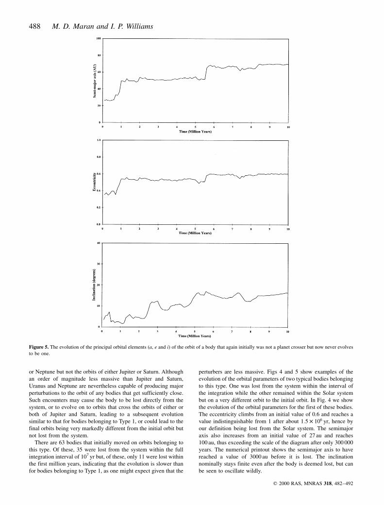
Figure 5. The evolution of the principal orbital elements (a, e and i) of the orbit of a body that again initially was not a planet crosser but now never evolves
to be one.
488 M. D. Maran and I. P. Williams
q 2000 RAS, MNRAS 318, 482±492
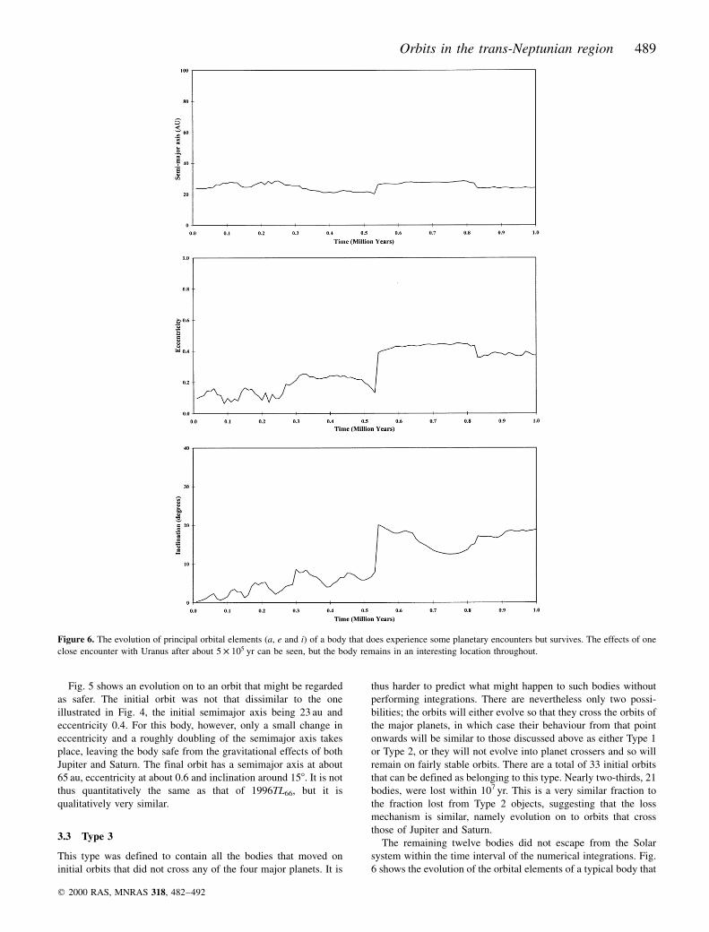
Fig. 5 shows an evolution on to an orbit that might be regarded
as safer. The initial orbit was not that dissimilar to the one
illustrated in Fig. 4, the initial semimajor axis being 23 au and
eccentricity 0.4. For this body, however, only a small change in
eccentricity and a roughly doubling of the semimajor axis takes
place, leaving the body safe from the gravitational effects of both
Jupiter and Saturn. The final orbit has a semimajor axis at about
65 au, eccentricity at about 0.6 and inclination around 158. It is not
thus quantitatively the same as that of 1996TL66, but it is
qualitatively very similar.
3.3 Type 3
This type was defined to contain all the bodies that moved on
initial orbits that did not cross any of the four major planets. It is
thus harder to predict what might happen to such bodies without
performing integrations. There are nevertheless only two possi-
bilities; the orbits will either evolve so that they cross the orbits of
the major planets, in which case their behaviour from that point
onwards will be similar to those discussed above as either Type 1
or Type 2, or they will not evolve into planet crossers and so will
remain on fairly stable orbits. There are a total of 33 initial orbits
that can be defined as belonging to this type. Nearly two-thirds, 21
bodies, were lost within 107 yr. This is a very similar fraction to
the fraction lost from Type 2 objects, suggesting that the loss
mechanism is similar, namely evolution on to orbits that cross
those of Jupiter and Saturn.
The remaining twelve bodies did not escape from the Solar
system within the time interval of the numerical integrations. Fig.
6 shows the evolution of the orbital elements of a typical body that
Figure 6. The evolution of principal orbital elements (a, e and i) of a body that does experience some planetary encounters but survives. The effects of one
close encounter with Uranus after about 5 � 105 yr can be seen, but the body remains in an interesting location throughout.
Orbits in the trans-Neptunian region 489
q 2000 RAS, MNRAS 318, 482±492
behaves in such a fashion. The initial orbit had a semimajor axis of
25 au and eccentricity of 0.1. Although there are changes in the
elements, they are not dramatic, though the effects of one close
encounter with Uranus after about 5:2 � 105 yr can be seen. After
this encounter, the body remains in an interesting location with the
semimajor axis remaining at about 23 au, the eccentricity at about
0.4 and the inclination at about 188. It has not, within the
integration time, however, evolved on to an orbit qualitatively
similar to that of 1996TL66, but further changes over a longer
time-scale may allow this to happen.
Two objects were initially on orbits that were far from all
planets and remained so for the full integration interval. Both
started on circular orbits at 25 and 26 au respectively. Within the
time interval of the integration, the semimajor axes evolved to
25.1 and 26.3 au respectively, while the eccentricities in the same
interval increased to 0.068 and 0.055, respectively. Thus both
orbits essentially remained at their initial values, though it is
dangerous to extrapolate and conclude that such behaviour persists
for the lifetime of the Solar system.
4 T H E P R O D U C T I O N O F I N T E R M E D I AT E -
T Y P E O R B I T S S U C H A S T H AT O F 1 9 9 6 T L 6 6
The only group of test objects that might fall into this category are
those objects that actually survived for the total period of the
integration. Three objects from Type 1 survived, but these were on
rather unique orbits and have been discussed already. None
actually evolved on to an orbit that might be termed promising
within this context. There were 28 bodies belonging to Type 2 and
12 belonging to Type 3 that survived for this time interval,
although two of these bodies belonging to Type 3 have also been
discussed already and can also be discounted from present
considerations. Hence, there are a possible 38 bodies from the
initial 210 that may evolve on to scattered orbits.
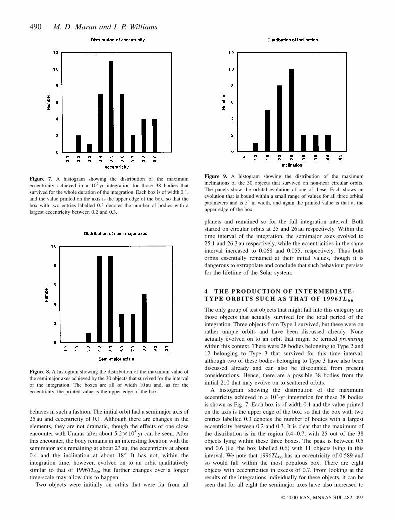
A histogram showing the distribution of the maximum
eccentricity achieved in a 107-yr integration for these 38 bodies
is shown as Fig. 7. Each box is of width 0.1 and the value printed
on the axis is the upper edge of the box, so that the box with two
entries labelled 0.3 denotes the number of bodies with a largest
eccentricity between 0.2 and 0.3. It is clear that the maximum of
the distribution is in the region 0.4±0.7, with 25 out of the 38
objects lying within these three boxes. The peak is between 0.5
and 0.6 (i.e. the box labelled 0.6) with 11 objects lying in this
interval. We note that 1996TL66 has an eccentricity of 0.589 and
so would fall within the most populous box. There are eight
objects with eccentricities in excess of 0.7. From looking at the
results of the integrations individually for these objects, it can be
seen that for all eight the semimajor axes have also increased to
Figure 9. A histogram showing the distribution of the maximum
inclinations of the 30 objects that survived on non-near circular orbits.
The panels show the orbital evolution of one of these. Each shows an
evolution that is bound within a small range of values for all three orbital
parameters and is 58 in width, and again the printed value is that at the
upper edge of the box.
Figure 7. A histogram showing the distribution of the maximum
eccentricity achieved in a 107 yr integration for those 38 bodies that
survived for the whole duration of the integration. Each box is of width 0.1,
and the value printed on the axis is the upper edge of the box, so that the
box with two entries labelled 0.3 denotes the number of bodies with a
largest eccentricity between 0.2 and 0.3.
Figure 8. A histogram showing the distribution of the maximum value of
the semimajor axes achieved by the 30 objects that survived for the interval
of the integration. The boxes are all of width 10 au and, as for the
eccentricity, the printed value is the upper edge of the box.
490 M. D. Maran and I. P. Williams
q 2000 RAS, MNRAS 318, 482±492
values in excess of 100 au, whereas this is not the case for any of
the other 30 bodies. These eight bodies are thus also likely to be
lost from the system, but 107 yr has not been quite long enough to
achieve this.
A histogram showing the distribution of the maximum value of
the semimajor axis achieved by these remaining 30 bodies during
the interval of the integration is shown as Fig. 8. The boxes are all
of width 10 au and, as for the eccentricity, the printed value is the
upper edge of the box. We note that all lie between 20 and 80 au,
the mean being about 50 au, somewhat smaller than the semimajor
axis of 1996TL66.
A histogram showing the distribution of the maximum
inclination achieved by these 30 objects can be seen in Fig. 9.
The boxes are 58 in width and again the printed value is that at the
upper edge of the box. Note that a certain distortion is caused by
this, because it hides the number of objects that are essentially in
the ecliptic. With this caveat, we note that the range of values of
the inclination displayed is very consistent with that observed for
trans-Neptunian objects, namely up to 388. 1996TL66 has an
inclination of 248, again very consistent with the model results. We
thus conclude that within this set of objects, which represent about
14 per cent of the initial set, a significant number of intermediate-type
bodies moving on orbits similar to that of 1996TL66 can be found.
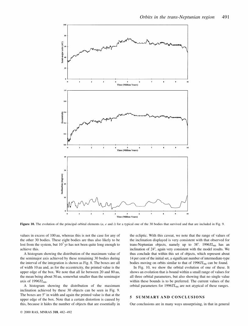
In Fig. 10, we show the orbital evolution of one of these. It
shows an evolution that is bound within a small range of values for
all three orbital parameters, but also showing that no single value
within these bounds is to be preferred. The current values of the
orbital parameters for 1996TL66 are not atypical of these ranges.
5 S U M M A RY A N D C O N C L U S I O N S
Our conclusions are in many ways unsurprising, in that in general
Figure 10. The evolution of the principal orbital elements (a, e and i) for a typical one of the 30 bodies that survived and that are included in Fig. 9.
Orbits in the trans-Neptunian region 491
q 2000 RAS, MNRAS 318, 482±492
the test particles behaved more or less as common sense would
lead us to expect. Of the 210 test particles placed on orbits
distributed in the manner that we have indicated in the previous
discussion, 177 had orbits that permitted very close approaches to
at least one of the four major planets and, unsurprisingly, all but
31 of them were lost from the system within the time-scale of the
integration, namely 107 yr. The remaining 33 test particles also
evolved in the generally expected way, with some evolving on to
planet-crossing orbits and others being on very stable near circular
orbits. Within the context of the original aim of this paper, namely
to generate orbits similar to 1996TL66, we note that 30 test
particles or 14 per cent evolved on to orbits that in some sense
could be classified as of this type.
R E F E R E N C E S
Dormand J. R., EI-Mikkai M. E. A., Prince P. J., 1987, IMA J. Numer.
Anal., 7, 423
Duncan M., Quinn T., Tremaine S., 1988, ApJ, 328, L69
Edgeworth K. E., 1943, J. Br. Astron. Assoc., 53, 181±188
Holman M. J., Wisdom J., 1993, AJ, 105, 1987
Jewitt D. C., Luu J. X., 1992, IAU Circ. 5611,
Kenyon S. J., Luu J. X., 1998, AJ, 115, 2136
Kuiper G. P., 1951, in Hynek J. A., eds, Astrophysics, A Topical
Symposium. McGraw-Hill, New York, p. 357
Luu J., Marsden B. G., Jewitt D., Trujillo C. A., Hergenrother C. W., 1997,
Nat, 387, 573
Oort P., 1950, Bull. Astron. Inst. Netherlands, 11, 91
Quinn T., Tremaine S., Duncan M., 1990, ApJ, 355, 667
Roy A. E.,et al., 1988, Vistas Astron., 32, 95
Stagg C. R., Bailey M. E., 1989, MNRAS, 421, 507
Stern S. A., 1996, AJ, 110, 1203
Trujillo C. A., Jewitt D. C., Luu J. X., 2000, ApJ, 529, L103
Williams I. P., O'Ceallaigh D. P., Fitzsimmons A., Marsden B. G., 1995,
Icarus, 116, 180
This paper has been typeset from a TEX/LATEX file prepared by the author.
492 M. D. Maran and I. P. Williams
q 2000 RAS, MNRAS 318, 482±492
Recommended