SCIENCE

The use of transformations in applyingboundary conditions to three-dimensional

vector field problemsD. Rodger, B.Sc.(Eng.), Ph.D., A.M.I.E.E., and Prof. J.F. Eastham, D.Sc,

Ph.D., C.Eng., F.I.E.E., F.R.S.(Edin.)

Indexing terms: Eddy currents, Electromagnetics

Abstract: A method for calculating three-dimensional eddy-current distributions has previously been described.It consists of using magnetic scalars to model fields in regions in which eddy currents do not flow, coupled to athree-component vector, the magnetic vector potential A, which describes the field inside eddy-current-carryingconductors. Applying boundary conditions to the region containing A is straightforward only in very simplecases. A technique for removing this limitation is described here. Results are substantiated by comparison withtwo test problems taken from the literature.

1 Introduction

A method for solving three-dimensional eddy-currentproblems in terms of coupled magnetic scalars and mag-netic vector potentials has already been described [1-6].The three-component vector A is used to model the fieldonly inside conductors in which eddy currents flow, whilemagnetic scalar potentials are used everywhere else in theproblem region.

In this way, a fairly economic description of a givenproblem may usually be obtained. While three degrees offreedom per node are required inside eddy regions, onlyone degree of freedom is necessary in nonconductingregions. The method should therefore compare favourablyin terms of both equation count and matrix sparsity withother possible approaches which require a vector fieldeverywhere, particularly in situations where the scalarregion is much larger than the vector region.

This method is especially convenient where it is used inconjunction with finite-element techniques, as all the inter-face conditions pertaining to the surfaces between thescalar and vector regions may then be readily handled.However, boundary conditions in the vector regions some-times warrant special treatment.

The usual Dirichlet or homogeneous Neumann bound-ary conditions can always be introduced to the magneticscalar potentials very simply, using standard techniques[7], whereas, in magnetic vector potential regions, theseboundary conditions can only be dealt with in the samestraightforward way if the boundary surface is planar andcan be conveniently aligned with the global Cartesian co-ordinates. Unfortunately, this is not possible in manyproblems.

A method for removing this limitation is described here.The technique consists of transforming the components ofthe boundary field variables from their global co-ordinatevalues to a more suitable local co-ordinate system in whichthe boundary condition may easily be applied. Analogousmethods have been used in other areas [7] but have notbeen applied to electromagnetic field problems. The pro-cedure is inexpensive and simple, often resulting in con-siderable savings in computational effort as all possiblesymmetry conditions may usually be exploited. The

Paper 3921A, (S8), first received 16th January 1984 and in revised form 15 March1985

The authors are with the School of Electrical Engineering, University of Bath, Cla-verton Down, Bath, United Kingdom

method is described here in terms of the coupled magneticvector-scalar potential method, but the same techniquecould profitably be applied to any other vector field for-mulation such as T - Q [8, 9].

The technique is verified by comparison with some testproblems taken from the literature. Eddy-current flow in ahollow spherical conducting shell [10] is calculated inSection 4.1 and a conducting-block problem [11] isaddressed in Section 4.2.

2 Field equations

2.1 Maxwell's equationsSince the mixed scalar and vector potential method hasbeen described elsewhere, only the details which have rele-vance to the present work will be reiterated.

Proceeding from the low-frequency limit of Maxwell'sequations, in which displacement currents are neglected,we have

curl E = —

curl H = J

div B = 0

div / = 0

dB

dt (1)

(2)

(3)

(4)

Also, we define the material properties in the usual way:

H=vB = B/n (5)

J=oE (6)

2.2 Fields in nonconducting regionsIf eddy-current flow in current sources can be neglected, amagnetic scalar potential <f> can be used to model part ofthe total field H, that is

H = - grad 4> + Hs (7)

where Hs is the field which is due to the source currents Js

only, so that curl Hs = Js. In this context $ is usuallyreferred to as the reduced scalar potential.

Unfortunately, the field derived from the reduced scalarpotential is opposed to that derived from the source cur-rents inside regions of high permeability, and this cancel-lation leads to a serious loss of accuracy as H is, in thesecircumstances, a relatively small quantity derived from thedifference of two much larger numbers.

1EE PROCEEDINGS, Vol. 132, Pt. A, No. 4, JULY 1985 165

However, in current-free regions where curl H = 0, thefield H can be completely represented by a magnetic scalarpotential

H = — grad \\i (8)

Clearly, eqn. 8 involves none of the cancellation difficultiesinherent in eqn. 7.

It was shown in Reference 12 that both potentials 0 and\j/ could be used together in magnetostatic problemswithout loss of accuracy, by first of all splitting theproblem region up in such a way that (j> is used insidesource current regions, and \j/ in iron regions, while either(f) or \\f could be applied everywhere else. This techniquehas also been found to be useful for modelling the mag-netic scalar potential regions of eddy-current problems.

By the Helmholtz theorem, descriptions of both thedivergence and curl are required in defining a uniquevector field. As the curl of the gradient of a scalar is alwayszero, eqns. 3 and 8, together with appropriate boundaryconditions, define a unique H\

div JX grad \j/ = 0 (9)

Eqn. 9 can be treated using Galerkin weighted residualtechniques to yield an alternative statement of the problem[7]:

\x grad N • grad if/dQ — N ^- dY = 0dn

(10)

in which N are three-dimensional shape functions. Thisequation leads directly to a standard finite-element solu-tion. A similar expression in 0 can be derived. Consider-ation of the continuity of tangential H and normal B at theinterface between (f> and \\i gives rise, eventually, to thesource terms for the field, as described in Reference 12.

2.3 Fields in eddy-current regionsThe field variation in eddy-current regions may bedescribed in terms of a magnetic vector potential A so that

curl A = B

From this and eqns. 1-6 we may derive

curl v curl A = \dA ^ 1~ ° \~dt + g ^ e

(11)

(12)

The electric scalar potential cpe can be shown to beredundant in this formulation [3] if the A — i// interfacecoincides exactly with conductor surfaces and if the con-ductivity is suitably well behaved. This implies that E andA are closely related:

(13)

Setting (j)e to zero in eqn. 12 and treating the resultingexpression in the same way as for eqn. 10, we have

I dAv curl TV • curl A + oN • — dQ

dt

- <pN • (v curl A x n) dY = 0 (14)

where TV = {Ni + Nj + Nk).This expression can be used in areas of discontinuous v.

If v is constant throughout the eddy region, it is convenientto first of all use a well known vector identity to expandthe left-hand side of eqn. 12, that is

Setting div A to zero in eqn. 15 (the Coulomb gauge) yieldsthe vector Poisson equation in A. Again, treating this asfor eqn. 10 yields

J[v grad N • grad Ax + No9AJdt]

dQ

dAv—^dY = 0 (16)

for the x component, the y and z expressions being similar.Where appropriate, that is if v is constant throughout

an A region, eqn. 16 should be used in place of eqn. 14 in asolution, as the former expression not only yields equa-tions which are about one third as dense as the latter atinterior nodes, but, in addition, the solution to the finalequation system can be found in fewer preconditionedbiconjugate gradient iterations than for the latter case. A,as defined by eqn. 16, is unique, as that equation impliesthat div A is zero. However, the divergence of a A is onlyspecified in eqn. 14 (as zero) when the o{dA)/(dt) term issufficiently large [6], so that, in some cases, additionalconstraints must be applied to eqn. 14. Lagrange multi-pliers were used in Reference 3.

2.4 Conditions at the A - if/ interfaceIf the equations in A and ij/ are linked together at the rele-vant interface nodes in such a way so as to ensure contin-uity of tangential H and normal B at the conductorsurfaces, this yields a unique system of linear equations tobe solved for A, ij/ and <j). This procedure is straightforwardand is carried out using the surface integral terms fromeqns. 10 for normal B and from eqn. 14 or eqn. 16 fortangential H [3].

3 Boundary conditions in vector regions

3.1 PreliminariesHomogeneous Neumann boundary conditions are naturalto the magnetic scalar potentials, due to the presence ofthe surface term as in eqn. 10. Dirichlet conditions areusually imposed at a node by means of simple operationson that particular row and column of the matrix, togetherwith the right-hand side of the equation system [7].

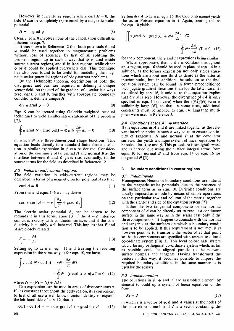
Either the two tangential components or the normalcomponent of A can be directly set to zero at a conductorsurface in the same way as in the scalar case only if thethree components of A happen to coincide with the normaland tangents at the surfaces on which a boundary condi-tion is to be applied. If this requirement is not met, it ishowever possible to transform the vector A at that pointso that its components are specified with respect to a localco-ordinate system (Fig. 1). This local co-ordinate systemwould be any orthogonal co-ordinate system which, as faras possible, could be aligned parallel to the relevantsurface normals and tangents. Having transformed thevectors in this way, it becomes possible to impose therequired boundary conditions in the same manner as isused for the scalars.

3.2 ImplementationThe equations in if/, 4> and A are assembled element byelement to build up a system of linear equations of theform

Kc = d (17)

curl v curl A = — v div grad A + v grad div A (15)in which c is a vector of 0, \j/ and A values at the nodes ofthe finite-element mesh and d is a vector containing the

166 IEE PROCEEDINGS, Vol. 132, Pt. A, No. 4, JULY 1985

sources of the problem (derived from simple functions ofthe Hs field on the </> — ij/ surface in a similar manner tothat which was described in Reference 12 for the magneto-static case). The matrix K is antisymmetric in the termswhich link A with the magnetic scalars. Typically thismatrix can be symmetrised by suitable multiplications by

node p

t

Fig. 1 A local co-ordinate system at node p

A = Axi + Agj + Azk

= Anii + Ass + A,t

n is the 'average' normal to the element surfaces which are connected to node p

cos e = im

y

Fig. 2A Conducting spherical shell in a uniform alternating magneticfield (Reference 10)

By

Fig. 2B Showing one 30° segment of a spherical shell

R0.02675 R0.0378 R0.02675 R0.03780 -*H -+A X_ 0

mesh ml mesh m2Fig. 3 Showing part of the two basic meshes for the spherical-conducting-shell problemBoth measure 0.2 m x 0.2 mDimensions in metres

— 1.0 at the assembly stage, so that only the upper orlower triangular part of K need be stored.

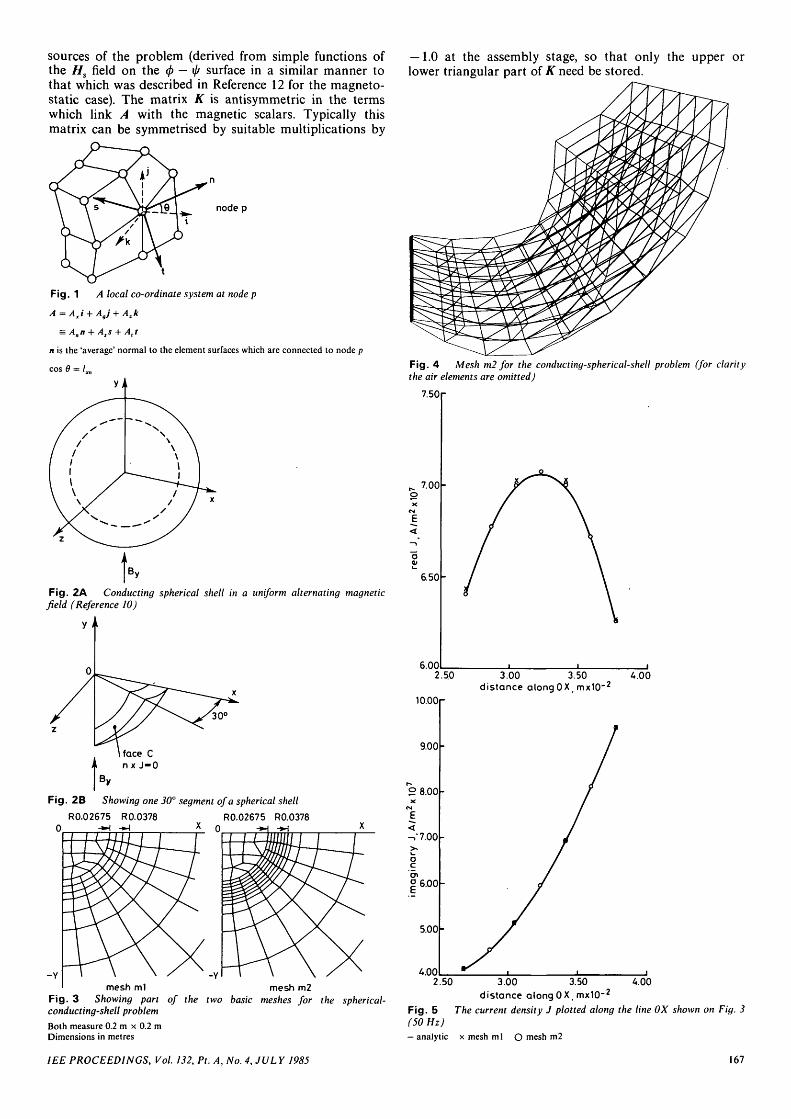
Fig. 4 Mesh m2 for the conducting-spherical-shell problem (for claritythe air elements are omitted)

7.50r

7.00

6.50

6.002.50 3.00 3.50

distance along0X/mx10"24.00

10.00r

9.00

2 8.00

V7.00

°6.00

5.00

4.002.50 3.00 3.50 4.00

distance along OX, mx10"2

The current density J plotted along the line OX shown on Fig. 3Fig. 5(50 Hz)— analytic x mesh ml O mesh m2

IEE PROCEEDINGS, Vol. 132, Pt. A, No. 4, JULY 1985 167

If the field A is represented at a node p by its threeorthogonal components in the global (x, y, z) co-ordinatesystem, then the same field may also be represented in anyother orthogonal co-ordinate system (n, s, t) rotated withrespect to (x, y, z), as

A' =

where

An

As

A= £10?

~AX'

Ay

Az_

(18)

I

j

k

= [L] P

n

s

t

and [L]P =

'jet

'zn '•zs '•zt

(19)

and in which /,,„ is the cosine of the angle between i and netc., as shown in Fig. 1. (Also, [L]£designates the matrix transpose.)

Clearly, from eqn. 17, we can obtain

KLc' = d

1.30r

1.20

1.10

1.00

0.90

^ 0.80o

0.70

0.60

0.50

0.40

0.30

= [L]p *, where T

(20)

0.20 0.40 0.60 0.80 1.00 1.20distance along OX mxiO"1

2.00r

1.00

o -1.00

1 -2.00

o£ -3.00enoE

-4.00

-5.00

-6.000 0.20 0.40 0.60 0.80 1.00 1.20

distance along OX mxiO"1

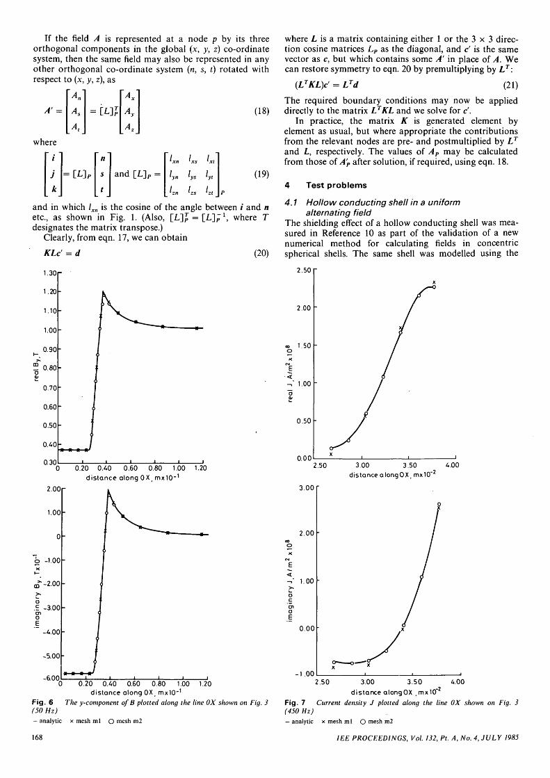
Fig. 6 The y-component of B plotted along the line OX shown on Fig. 3(50 Hz)— analytic x mesh ml O mesh m2

168

where L is a matrix containing either 1 or the 3 x 3 direc-tion cosine matrices LP as the diagonal, and c' is the samevector as c, but which contains some A' in place of A. Wecan restore symmetry to eqn. 20 by premultiplying by LT:

(LTKL)c' = LTd (21)

The required boundary conditions may now be applieddirectly to the matrix LTKL and we solve for c'.

In practice, the matrix K is generated element byelement as usual, but where appropriate the contributionsfrom the relevant nodes are pre- and postmultiplied by LT

and L, respectively. The values of AP may be calculatedfrom those of A'P after solution, if required, using eqn. 18.

Test problems

4.1 Hollow conducting shell in a uniformalternating field

The shielding effect of a hollow conducting shell was mea-sured in Reference 10 as part of the validation of a newnumerical method for calculating fields in concentricspherical shells. The same shell was modelled using the

2 .50r

2.00

1.50

," 1.00

0.50

0.002.50

3.00T

2.00

1.00

0.00

3.00 3.50 4.00distance alongOX. mx10"

-1.002.50 3.00 3.50 4.00

distance along OX ,mx10"Fig. 7 Current density J plotted along the line OX shown on Fig. 3(450 Hz)— analytic x mesh ml O mesh m2

1EE PROCEEDINGS, Vol. 132, Pt. A, No. 4, JULY 1985

method outlined here. The field quantities were, however,compared with those obtained from the classical analyticsolution, so as to avoid the situation in which one numeri-cal method is compared with another. In passing it wasobserved that the results obtained previously [10] didshow very good correspondence with the analytic solution.

Figs. 2A and 2B shows the conducting shell, inner andouter radius 26.75 and 37.8 mm, respectively. The shellconductivity is 2.65 x 107 Sm"1 and it is immersed in aspatially uniform, time sinusoidally varying, magnetic fieldof infinite extent (By = IT). The permeability is n0

throughout the whole region.Two meshes were used to model the shell, which were

generated by rotating the meshed planes (shown as ml andm2 on Fig. 3) about the line 07, to form six noded iso-parametric wedge-shaped elements along 0 7 and eightnoded isoparametric brick-shaped elements everywhereelse. Two 30° segments were formed in this way, each con-sisting of two 15° segments (m2 is shown in Fig. 4). Onesegment would have been sufficient for a solution, but itwas thought important to retain a model in which all threecomponents of A were represented for the purposes of this

1.40

1.30

1.20

1.10

1.00

0.90

0.80

0.70

»-. 0.60

crT 0.50

2 0.40

0.30

0.20

0.10

0.00

-0.10

\

000 0.20 0.40 0.60distance along OX ,mx10

0.80 "1.00-1

1.20

1.00

-0.00

7 -1.00o

CD - 2 . 0 0

en

9 -3.00

-4.00

-5.00

^6-6-6,

o

I0.00 0.20 0.40 0.60 0.80 1.00 120

distance along OX , mxiO"1

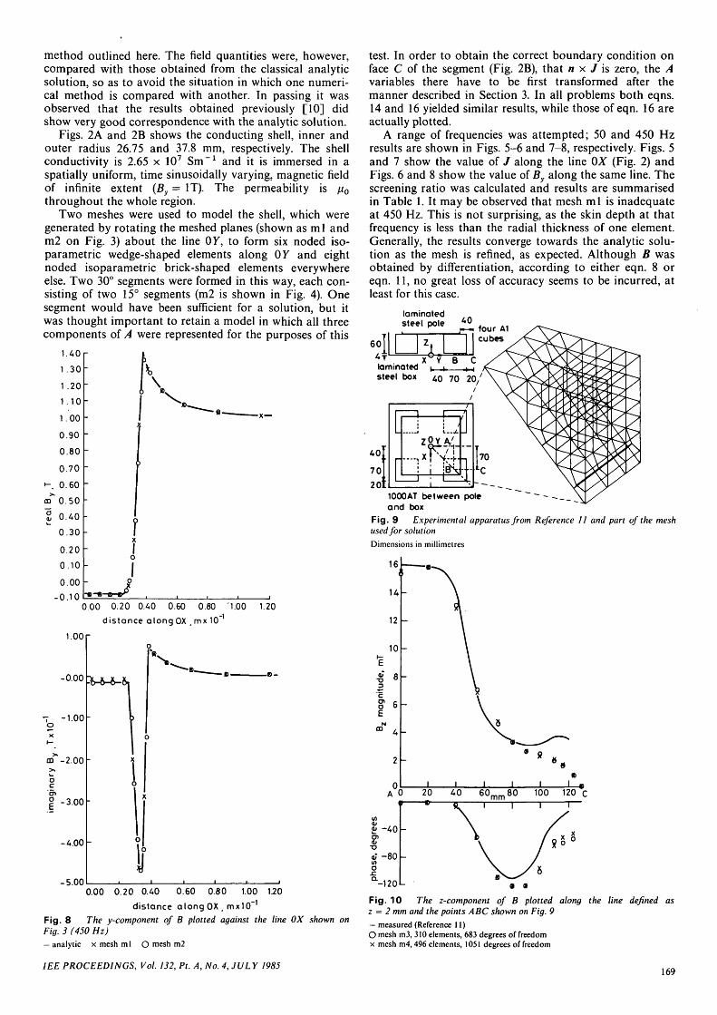
Fig. 8 The y-component of B plotted against the line OX shown onFig. 3 (450 Hz)— analytic x mesh ml O mesh m2

test. In order to obtain the correct boundary condition onface C of the segment (Fig. 2B), that n x J is zero, the Avariables there have to be first transformed after themanner described in Section 3. In all problems both eqns.14 and 16 yielded similar results, while those of eqn. 16 areactually plotted.

A range of frequencies was attempted; 50 and 450 Hzresults are shown in Figs. 5-6 and 7-8, respectively. Figs. 5and 7 show the value of J along the line OX (Fig. 2) andFigs. 6 and 8 show the value of By along the same line. Thescreening ratio was calculated and results are summarisedin Table 1. It may be observed that mesh ml is inadequateat 450 Hz. This is not surprising, as the skin depth at thatfrequency is less than the radial thickness of one element.Generally, the results converge towards the analytic solu-tion as the mesh is refined, as expected. Although B wasobtained by differentiation, according to either eqn. 8 oreqn. 11, no great loss of accuracy seems to be incurred, atleast for this case.

laminatedsteel pole 40

60 ZI

four A1cubes

laminated X Y

steel box 4 0 70 20/

1000AT between pole ~ "~ - - _and box

Fig. 9 Experimental apparatus from Reference 11 and part of the meshused for solution

Dimensions in millimetres

Fig. 10 The z-component of B plotted along the line defined asz = 2 mm and the points ABC shown on Fig. 9— measured (Reference 11)O mesh m3, 310 elements, 683 degrees of freedomx mesh m4,496 elements, 1051 degrees of freedom

IEE PROCEEDINGS, Vol. 132, Pi. A, No. 4, JULY 1985169

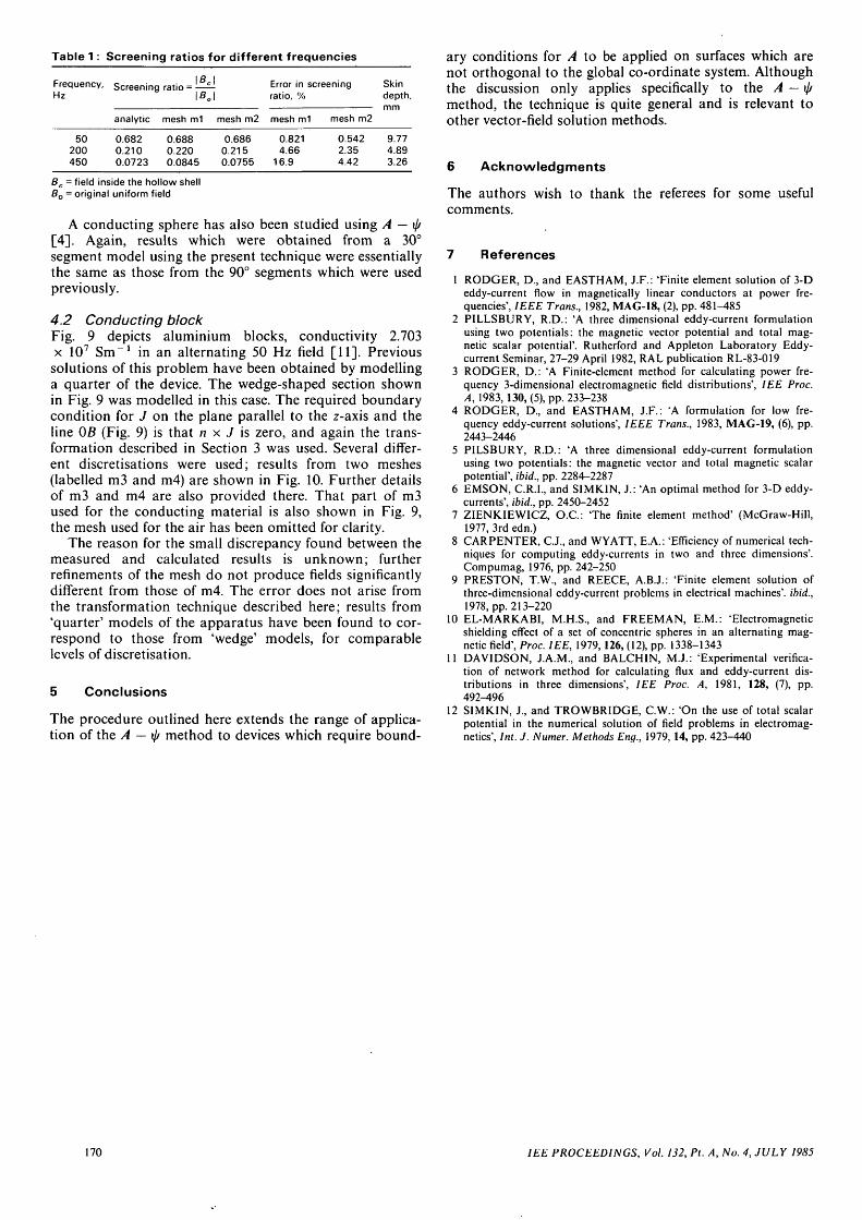
Table 1 : Screening ratios for different frequencies

Frequency,Hz

50200450

Screening

analytic

0.6820.2100.0723

. \Beratio =

\BO

mesh ml

0.6880.2200.0845

II

mesh m2

0.6860.2150.0755

Error in screeningratio, %

mesh ml

0.8214.66

16.9

mesh m2

0.5422.354.42

Skindepth,mm

9.774.893.26

Bc = field inside the hollow shellBo = original uniform field

A conducting sphere has also been studied using A — \j/[4]. Again, results which were obtained from a 30°segment model using the present technique were essentiallythe same as those from the 90° segments which were usedpreviously.

4.2 Conducting blockFig. 9 depicts aluminium blocks, conductivity 2.703x 107 Sm"1 in an alternating 50 Hz field [11]. Previoussolutions of this problem have been obtained by modellinga quarter of the device. The wedge-shaped section shownin Fig. 9 was modelled in this case. The required boundarycondition for J on the plane parallel to the z-axis and theline 0B (Fig. 9) is that n x J is zero, and again the trans-formation described in Section 3 was used. Several differ-ent discretisations were used; results from two meshes(labelled m3 and m4) are shown in Fig. 10. Further detailsof m3 and m4 are also provided there. That part of m3used for the conducting material is also shown in Fig. 9,the mesh used for the air has been omitted for clarity.

The reason for the small discrepancy found between themeasured and calculated results is unknown; furtherrefinements of the mesh do not produce fields significantlydifferent from those of m4. The error does not arise fromthe transformation technique described here; results from'quarter' models of the apparatus have been found to cor-respond to those from 'wedge' models, for comparablelevels of discretisation.

5 Conclusions

The procedure outlined here extends the range of applica-tion of the A — \jj method to devices which require bound-

ary conditions for A to be applied on surfaces which arenot orthogonal to the global co-ordinate system. Althoughthe discussion only applies specifically to the A — ^method, the technique is quite general and is relevant toother vector-field solution methods.

6 Acknowledgments

The authors wish to thank the referees for some usefulcomments.

7 References

1 RODGER, D., and EASTHAM, J.F.: 'Finite element solution of 3-Deddy-current flow in magnetically linear conductors at power fre-quencies', IEEE Trans., 1982, MAG-18, (2), pp. 481-485

2 PILLSBURY, R.D.: 'A three dimensional eddy-current formulationusing two potentials: the magnetic vector potential and total mag-netic scalar potential'. Rutherford and Appleton Laboratory Eddy-current Seminar, 27-29 April 1982, RAL publication RL-83-019

3 RODGER, D.: 'A Finite-element method for calculating power fre-quency 3-dimensional electromagnetic field distributions', IEE Proc.A, 1983, 130, (5), pp. 233-238

4 RODGER, D., and EASTHAM, J.F.: 'A formulation for low fre-quency eddy-current solutions', IEEE Trans., 1983, MAG-19, (6), pp.2443-2446

5 PILSBURY, R.D.: 'A three dimensional eddy-current formulationusing two potentials: the magnetic vector and total magnetic scalarpotential', ibid., pp. 2284-2287

6 EMSON, C.R.I., and SIMKIN, J.: 'An optimal method for 3-D eddy-currents', ibid., pp. 2450-2452

7 ZIENKIEWICZ, O.C.: 'The finite element method' (McGraw-Hill,1977, 3rd edn.)

8 CARPENTER, C.J., and WYATT, E.A.: 'Efficiency of numerical tech-niques for computing eddy-currents in two and three dimensions'.Compumag, 1976, pp. 242-250

9 PRESTON, T.W., and REECE, A.B.J.: 'Finite element solution ofthree-dimensional eddy-current problems in electrical machines', ibid.,1978, pp. 213-220

10 EL-MARKABI, M.H.S., and FREEMAN, E.M.: 'Electromagneticshielding effect of a set of concentric spheres in an alternating mag-netic field', Proc. IEE, 1979,126, (12), pp. 1338-1343

11 DAVIDSON, J.A.M., and BALCHIN, M.J.: 'Experimental verifica-tion of network method for calculating flux and eddy-current dis-tributions in three dimensions', IEE Proc. A, 1981, 128, (7), pp.492-496

12 SIMKIN, J., and TROWBRIDGE, C.W.: 'On the use of total scalarpotential in the numerical solution of field problems in electromag-netics', Int. J. Numer. Methods Eng., 1979, 14, pp. 423-440

170 IEE PROCEEDINGS, Vol. 132, Pt. A, No. 4, JULY 1985