Pecora 20 - Observing a Changing Earth; Science for Decisions— Monitoring, Assessment, and Projection
November 13-16, 2017 Sioux Falls, SD
WORLDVIEW-3 SWIR LAND USE-LAND COVER MINERAL CLASSIFICATION:
CUPRITE, NEVADA
K.E. Johnson, Staff R&D Scientist
K. Koperski, Principal R&D Scientist
DigitalGlobe, Inc.,
1300 W 120th Avenue,
Westminster, CO 80234
ABSTRACT
Cuprite, Nevada is a location well known for numerous studies of the hydrothermal mineralogy. In particular this
region has been used to validate geological interpretations of airborne hyperspectral (AVIRIS HSI), Advanced
Spaceborne Thermal Emission and Reflection Radiometer (ASTER) and 8-band satellite SWIR (WorldView-3)
imagery. WorldView-3 (WV-3) launched in August 2014, is a high-spatial resolution commercial multispectral
satellite sensor with eight visible to near infrared (VNIR) bands (0.42 to 1.04 m) and eight shortwave infrared (SWIR)
bands (1.2 to 2.33 m). Previous geological studies (Kruse et al., 2015) of WV-3 imagery at Cuprite, Nevada,
demonstrated the mineral identification and mapping capabilites of the 8-SWIR bands compared to hyperspectral data
(AVIRIS HSI) and ASTER. That study applied Mixture-Tuned-Matched-Filtering (MTMF) analysis. We have
applied Land Use-Land Cover (LULC) methods to all 16-bands of data, to perform a geological analysis of WV-3
satellite imagery of the Cuprite, Nevada location. We use the same imagery as the previous WV-3 studies at Cuprite
to facilitate the direct comparison of results. The VNIR (1.2 m) and SWIR (7.5m) images were co-registered into a
16-band layer stack for analysis. Ground truth for LULC training and validation was derived from AVIRIS
Hyperspectral data and USGS mineral spectral data for this location. We present the results of a supervised LULC
classification applying the Random Forest Decision Tree Algorithm with 20 trees. Seven geological materials were
tested for identification: Alunite, Calcite, Iron Oxides, Kaolinite, Muscovite, Palagonite (basaltic glass) and Silica
(var. chalcedony) with an accuracy of 84% and a kappa coefficient of 0.81 using the DigitalGlobe LULC Web
Application. The DG LULC Application includes Gabor Texture, Histogram and Mean values in the analysis. Support
Vector Machine Analysis (SPSS-SVM) yields a similar accuracy of 84%. Our experiments show the importance of
feature selection for the SVM classifier, while the Tree Classifiers are less sensitive with respect to features. Our
results show that with good ground truth, World View-3 SWIR + VNIR imagery produces an accurate geological
assessment.
KEYWORDS: WorldView-3, SWIR, Land Use-Land Cover Classification, Cuprite, Mineralogy
INTRODUCTION
WorldView-3 (WV-3), launched in August 2014 by DigitalGlobe, Inc (Westminster, Colorado) is the only
16-band commercial high-resolution Earth imaging satellite currently in orbit. In addition to the 8 visible and near
infrared (VNIR: 0.42 to 1.04 µm) bands, WV-3 has the expanded capability of 8 shortwave infrared bands (SWIR:
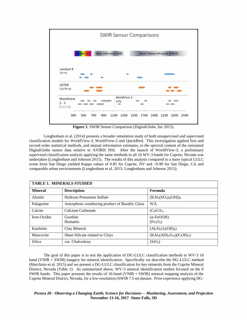
1.2 to 2.33 µm). The WV-3 SWIR band sensors (Figure 1) were carefully selected to provide remote mineral mapping
and materials identification capabilities not available in any other space-borne multispectral system (Kruse et al. 2015).
Previous studies by Kruse et al. (2015) and Kruse and Perry (2013) have tested WV-3 SWIR bands only. Both studies
applied the Mixture Tuned Matched Filtering (MTMF) method commonly used in AVIRIS classifications. Prior to
the launch of WV-3, Kruse and Perry (2013) compared simulated WV-3 data to Cuprite AVIRIS hyperspectral
imagery (HSI) and ASTER 6-band 30 m resolution SWIR imagery. Their preliminary findings suggested that WV-3
SWIR bands could be a significant tool for geologic mapping. Following the launch of WV-3, Kruse et al (2015)
provided a follow-up study using actual WV-3 SWIR data. This study again compared WV-3 SWIR to AVIRIS HSI,
reporting a WV-3 accuracy of 63.23% and Kappa = 0.51, and confirming the predicted mineral identification accuracy
of their earlier study.
Pecora 20 - Observing a Changing Earth; Science for Decisions— Monitoring, Assessment, and Projection
November 13-16, 2017 Sioux Falls, SD
Figure 1. SWIR Sensor Comparison (DigitalGlobe, Inc 2015).
Longbotham et al. (2014) presents a broader simulation study of both unsupervised and supervised
classification models for WorldView-3, WorldView-2 and QuickBird. This investigation applied first and
second order statistical methods, and mutual information estimates, to the spectral content of the simulated
DigitalGlobe sensor data relative to AVIRIS HSI. After the launch of WorldView-3, a preliminary
supervised classification analysis applying the same methods to all 16 WV-3 bands for Cuprite, Nevada was
undertaken (Longbotham and Johnson 2015). The results of this analysis compared to a more typical LULC
scene from San Diego yielded Kappa values of 0.85 for Cuprite, NV and >0.90 for San Diego, CA and
comparable urban environments (Longbotham et al. 2015; Longbotham and Johnson 2015).
TABLE 1. MINERALS STUDIED
Mineral Description Formula
Alunite Hydrous Potassium Sulfate (KAl3(SO4)2(OH))6
Palagonite Amorphous weathering product of Basaltic Glass N/A
Calcite Calcium Carbonate (CaCO3)
Iron-Oxides Goethite
Hematite
(α-FeOOH)
(Fe2O3)
Kaolinite Clay Mineral (Al2Si2O5(OH)4)
Muscovite Sheet Silicate related to Clays (KAl2(AlSi3O10)(F,OH)2)
Silica var. Chalcedony (SiO2)
The goal of this paper is to test the application of DG-LULC classification methods to WV-3 16
band (VNIR + SWIR) imagery for mineral identification. Specifically we describe the DG-LULC method
(Marchisio et al. 2015) and we present a DG-LULC classification for key minerals from the Cuprite Mineral
District, Nevada (Table 1). As summarized above, WV-3 mineral identification studies focused on the 8
SWIR bands. This paper presents the results of 16-band (VNIR + SWIR) mineral mapping analysis of the
Cuprite Mineral District, Nevada, for a low-resolution (SWIR 7.5 m) dataset. Prior experience applying DG-
Pecora 20 - Observing a Changing Earth; Science for Decisions— Monitoring, Assessment, and Projection
November 13-16, 2017 Sioux Falls, SD
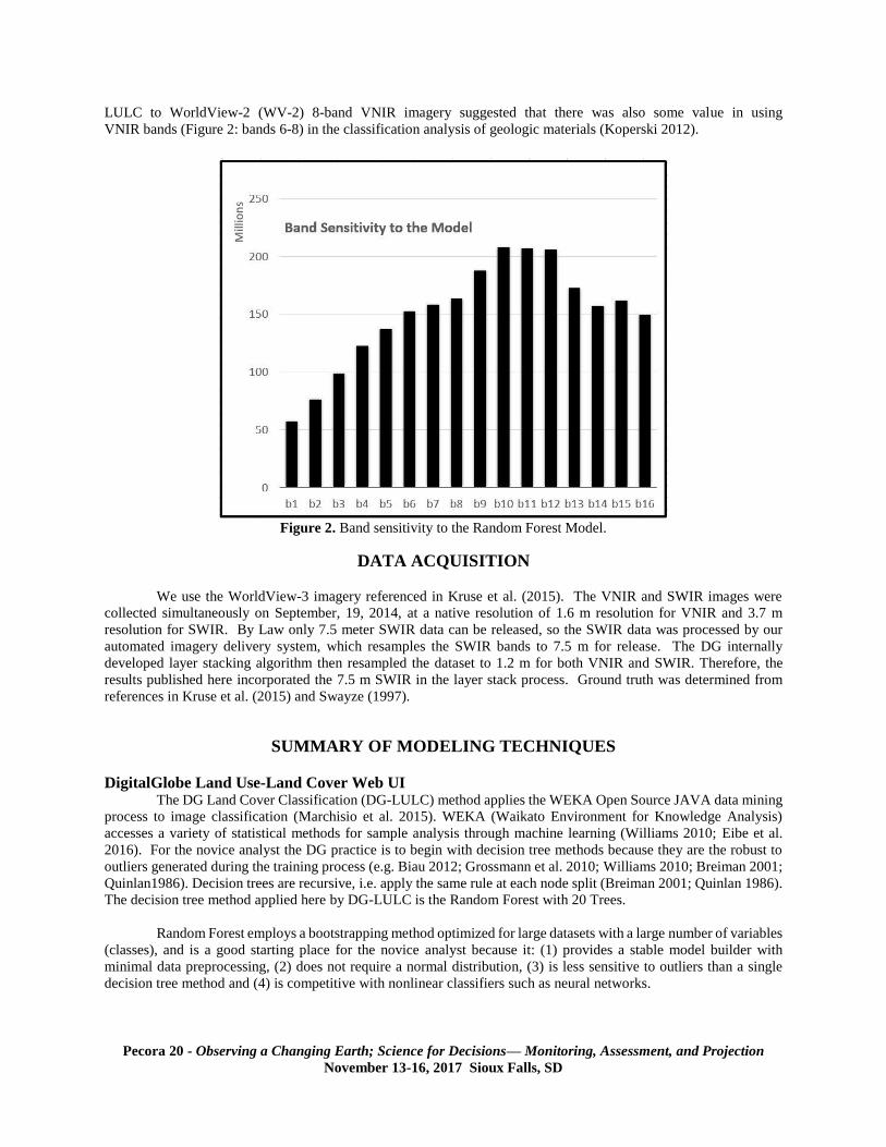
LULC to WorldView-2 (WV-2) 8-band VNIR imagery suggested that there was also some value in using
VNIR bands (Figure 2: bands 6-8) in the classification analysis of geologic materials (Koperski 2012).
Figure 2. Band sensitivity to the Random Forest Model.
DATA ACQUISITION
We use the WorldView-3 imagery referenced in Kruse et al. (2015). The VNIR and SWIR images were
collected simultaneously on September, 19, 2014, at a native resolution of 1.6 m resolution for VNIR and 3.7 m
resolution for SWIR. By Law only 7.5 meter SWIR data can be released, so the SWIR data was processed by our
automated imagery delivery system, which resamples the SWIR bands to 7.5 m for release. The DG internally
developed layer stacking algorithm then resampled the dataset to 1.2 m for both VNIR and SWIR. Therefore, the
results published here incorporated the 7.5 m SWIR in the layer stack process. Ground truth was determined from
references in Kruse et al. (2015) and Swayze (1997).
SUMMARY OF MODELING TECHNIQUES
DigitalGlobe Land Use-Land Cover Web UI The DG Land Cover Classification (DG-LULC) method applies the WEKA Open Source JAVA data mining
process to image classification (Marchisio et al. 2015). WEKA (Waikato Environment for Knowledge Analysis)
accesses a variety of statistical methods for sample analysis through machine learning (Williams 2010; Eibe et al.
2016). For the novice analyst the DG practice is to begin with decision tree methods because they are the robust to
outliers generated during the training process (e.g. Biau 2012; Grossmann et al. 2010; Williams 2010; Breiman 2001;
Quinlan1986). Decision trees are recursive, i.e. apply the same rule at each node split (Breiman 2001; Quinlan 1986).
The decision tree method applied here by DG-LULC is the Random Forest with 20 Trees.
Random Forest employs a bootstrapping method optimized for large datasets with a large number of variables
(classes), and is a good starting place for the novice analyst because it: (1) provides a stable model builder with
minimal data preprocessing, (2) does not require a normal distribution, (3) is less sensitive to outliers than a single
decision tree method and (4) is competitive with nonlinear classifiers such as neural networks.
Pecora 20 - Observing a Changing Earth; Science for Decisions— Monitoring, Assessment, and Projection
November 13-16, 2017 Sioux Falls, SD
DG-LULC employs training and validation datasets to initiate each node. Once a tree is completed
the next tree is initiated, until all have reached a conclusion. Each node is tested by the percent error of
misclassification of the validation dataset (Breiman 2001). The number of decision trees must be specified
and can range up to 1000 for very large data sets, with 500 as an average number of trees (Grossmann et al.
2010; Williams 2010). For the very small data sets, as for this study, 20 trees were specified for seven (7)
mineral classes. In image classification, the Random Forest method can be subject to bias if care has not
been taken to select balanced sample sizes amongst the training classes, and for both training and validation
datasets (Grossman et al. 2010). The Random Forest method, e.g., has been applied to Landsat data to
generate the USGS GAP Land Cover layers (Grossmann et al. 2010). For the details of the Random Forest
method, refer to Breiman (2001).
IBM-SPSS Support Vector Machine (SVM) & C5.0 Analysis Support Vector Machines (SVM) work by mapping data to a high-dimensional feature space so
that data points can be categorized, even when the data are not otherwise linearly separable (IBM SPSS
2017). A separator between the categories is found, the data are then transformed in such a way that the
separator could be drawn as a hyperplane. Following this, characteristics of new data can be used to predict
the group to which a new record should belong (IBM SPSS 2017). As a classifier, SVM models analyze
data and can recognize patterns that distinguish classes for small sample sets (Pandya and Pandya 2015).
C5.0 can produce two types of models: a decision tree or a rule set. In either mode, C5.0 splits the
sample based on the fields that provide the maximum normalized information gain (IBM SPSS 2017). As a
classifier it can anticipate which attributes are relevant and which are not relevant in the classification
(Pandya and Pandya 2015). Large decision trees can be pruned and simplified using rule sets which retain
most of the information of the original decision tree (IBM SPSS 2017). Given that our model inputs the data
from the DG-LULC Random Forest of 20 trees, only the decision tree mode was applied.
RESULTS AND DISCUSSION
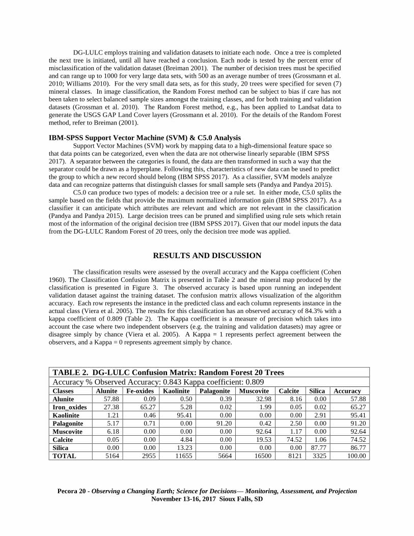
The classification results were assessed by the overall accuracy and the Kappa coefficient (Cohen
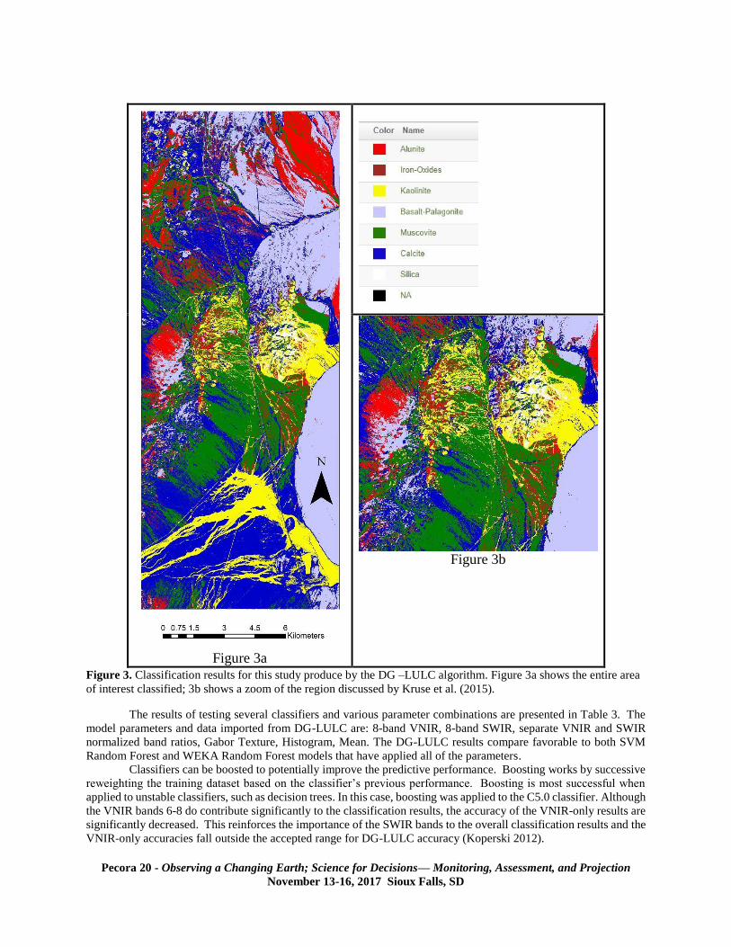
1960). The Classification Confusion Matrix is presented in Table 2 and the mineral map produced by the
classification is presented in Figure 3. The observed accuracy is based upon running an independent
validation dataset against the training dataset. The confusion matrix allows visualization of the algorithm
accuracy. Each row represents the instance in the predicted class and each column represents instance in the
actual class (Viera et al. 2005). The results for this classification has an observed accuracy of 84.3% with a
kappa coefficient of 0.809 (Table 2). The Kappa coefficient is a measure of precision which takes into
account the case where two independent observers (e.g. the training and validation datasets) may agree or
disagree simply by chance (Viera et al. 2005). A Kappa = 1 represents perfect agreement between the
observers, and a Kappa = 0 represents agreement simply by chance.
TABLE 2. DG-LULC Confusion Matrix: Random Forest 20 Trees
Accuracy % Observed Accuracy: 0.843 Kappa coefficient: 0.809 Classes Alunite Fe-oxides Kaolinite Palagonite Muscovite Calcite Silica Accuracy
Alunite 57.88 0.09 0.50 0.39 32.98 8.16 0.00 57.88
Iron_oxides 27.38 65.27 5.28 0.02 1.99 0.05 0.02 65.27
Kaolinite 1.21 0.46 95.41 0.00 0.00 0.00 2.91 95.41
Palagonite 5.17 0.71 0.00 91.20 0.42 2.50 0.00 91.20
Muscovite 6.18 0.00 0.00 0.00 92.64 1.17 0.00 92.64
Calcite 0.05 0.00 4.84 0.00 19.53 74.52 1.06 74.52
Silica 0.00 0.00 13.23 0.00 0.00 0.00 87.77 86.77
TOTAL 5164 2955 11655 5664 16500 8121 3325 100.00
Pecora 20 - Observing a Changing Earth; Science for Decisions— Monitoring, Assessment, and Projection
November 13-16, 2017 Sioux Falls, SD
Figure 3a
Figure 3b
Figure 3. Classification results for this study produce by the DG –LULC algorithm. Figure 3a shows the entire area
of interest classified; 3b shows a zoom of the region discussed by Kruse et al. (2015).
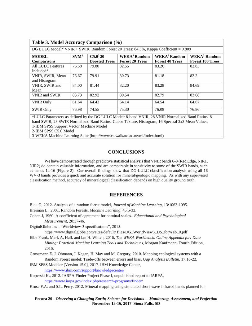
The results of testing several classifiers and various parameter combinations are presented in Table 3. The
model parameters and data imported from DG-LULC are: 8-band VNIR, 8-band SWIR, separate VNIR and SWIR
normalized band ratios, Gabor Texture, Histogram, Mean. The DG-LULC results compare favorable to both SVM
Random Forest and WEKA Random Forest models that have applied all of the parameters.
Classifiers can be boosted to potentially improve the predictive performance. Boosting works by successive
reweighting the training dataset based on the classifier’s previous performance. Boosting is most successful when
applied to unstable classifiers, such as decision trees. In this case, boosting was applied to the C5.0 classifier. Although
the VNIR bands 6-8 do contribute significantly to the classification results, the accuracy of the VNIR-only results are
significantly decreased. This reinforces the importance of the SWIR bands to the overall classification results and the
VNIR-only accuracies fall outside the accepted range for DG-LULC accuracy (Koperski 2012).
Pecora 20 - Observing a Changing Earth; Science for Decisions— Monitoring, Assessment, and Projection
November 13-16, 2017 Sioux Falls, SD
Table 3. Model Accuracy Comparison (%)
DG LULC Model* VNIR + SWIR, Random Forest 20 Trees: 84.3%, Kappa Coefficient = 0.809
MODEL
Comparisons
SVM1 C5.02 20
Boosted Trees
WEKA3 Random
Forest 20 Trees
WEKA3 Random
Forest 40 Trees
WEKA3 Random
Forest 100 Trees
All LULC Features
Included*
76.58 79.80 82.55 83.26 82.83
VNIR, SWIR, Mean
and Histogram
76.67 79.91 80.73 81.18 82.2
VNIR, SWIR and
Mean
84.00 81.44 82.20 83.28 84.69
VNIR and SWIR 83.73 82.92 80.54 82.79 83.68
VNIR Only 61.64 64.43 64.14 64.54 64.67
SWIR Only 76.98 74.55 75.30 76.08 76.86
*LULC Parameters as defined by the DG LULC Model: 8-band VNIR, 28 VNIR Normalized Band Ratios, 8-
band SWIR, 28 SWIR Normalized Band Ratios, Gabor Texture, Histogram, 16 Spectral 3x3 Mean Values.
1-IBM SPSS Support Vector Machine Model
2-IBM SPSS C5.0 Model
3-WEKA Machine Learning Suite (http://www.cs.waikato.ac.nz/ml/index.html)
CONCLUSIONS
We have demonstrated through predictive statistical analysis that VNIR bands 6-8 (Red Edge, NIR1,
NIR2) do contain valuable information, and are comparable in sensitivity to some of the SWIR bands, such
as bands 14-16 (Figure 2). Our overall findings show that DG-LULC classification analysis using all 16
WV-3 bands provides a quick and accurate solution for mineral/geologic mapping. As with any supervised
classification method, accuracy of mineralogical classification depends on high quality ground truth.
REFERENCES
Biau G, 2012. Analysis of a random forest model, Journal of Machine Learning, 13:1063-1095.
Breiman L., 2001. Random Forests, Machine Learning, 45:5-32.
Cohen J, 1960. A coefficient of agreement for nominal scales. Educational and Psychological
Measurement, 20:37-46.
DigitalGlobe Inc., “Worldview-3 specifications”, 2015.
https://www.digitalglobe.com/sites/default/ files/DG_WorldView3_DS_forWeb_0.pdf
Eibe Frank, Mark A. Hall, and Ian H. Witten, 2016. The WEKA Workbench. Online Appendix for: Data
Mining: Practical Machine Learning Tools and Techniques, Morgan Kaufmann, Fourth Edition,
2016.
Grossmann E. J. Ohmann, J. Kagan, H. May and M. Gregory, 2010. Mapping ecological systems with a
Random Forest model: Trade-offs between errors and bias, Gap Analysis Bulletin, 17:16-22.
IBM SPSS Modeler [Version 15.0], 2017. IBM Knowledge Center,
https://www.ibm.com/support/knowledgecenter/
Koperski K., 2012. IARPA Finder Project Phase I, unpublished report to IARPA,
https://www.iarpa.gov/index.php/research-programs/finder/
Kruse F.A. and S.L. Perry, 2012. Mineral mapping using simulated short-wave-infrared bands planned for
Pecora 20 - Observing a Changing Earth; Science for Decisions— Monitoring, Assessment, and Projection
November 13-16, 2017 Sioux Falls, SD
DigitalGlobe WorldView-3, in Proc. Imaging and Applied Optics Technical Digest, Monterey,
California, Paper RM3E.4.pdf (CD-ROM), Optical Society of America, Washington, D. C.
Kruse F.A., W.M. Baugh and S.L. Perry, 2015. Validation of DigitalGlobe WorldView-3 Earth imaging
satellite shortwave infrared bands for mineral mapping. Journal of Applied Remote Sensing,
9: 1-17.
Longbotham N. and K.E. Johnson, 2015. Unpublished data.
Longbotham N., F. Pacifici, S. Malitz, W. Baugh, G. Camps-Valls, 2015. Measuring the Spatial and
Spectral Performance of WorldView-3, in Hyperspectral Imaging and Sounding of the Environment
(HISE), 2015.
Longbotham N., F. Pacifici, W.M. Baugh and G. Camps-Valis 2014. Prelaunch assessment of
WorldView-3 information content, Workshop on Hyperstectral Image and Signal Processing: Evolution in
Remote Sensing, WHISPERS, Lausanne, Switzerland, https://www.researchgate.net/publication/283876097
Marchisio G.B., C. Tusk, K. Koperski, M.D. Tabb and J.D. Shafer, 2015. Classification of land based on
analysis of remotely-sensed earth images, DigitalGlobe, Inc: US Patent #9147132 B2
Pandya R. and J. Pandya, 2015. C5.0 algorithm to improved decision tree with feature selection and
reduced error pruning. International Journal of Computer Applications, 117: 18-21.
Quinlan J.R., 1986. Induction of decision trees, Machine Learning, 1:81-106.
Swayze G.A., 1997. The hydrothermal and structural history of the Cuprite Mining District, southwestern Nevada:
an integrated geological and geophysical approach, unpublished Ph.D. Dissertation, Univ. of Colorado at
Boulder, pp. 399, Boulder, Colorado.
Williams G., 2010. Data mining desktop survival guide, https://www.togaware.com/datamining/survivor/
Recommended