Download pdf - Zain 333343

1. Introduction to Probability

In some areas, such as mathematics or logic, results of some process can be known with certainty (e.g.,

2+3=5). Most real life situations, however, involve variability and uncertainty. For example, it is

uncertain whether it will rain tomorrow; the price of a given stock a week from today is uncertain

Note_1 ; the number of claims that a car insurance policy holder will make over a one-year period is

uncertain. Uncertainty or "randomness" (meaning variability of results) is usually due to some mixture of

two factors: (1) variability in populations consisting of animate or inanimate objects (e.g., people vary in

size, weight, blood type etc.), and (2) variability in processes or phenomena (e.g., the random selection

of 6 numbers from 49 in a lottery draw can lead to a very large number of different outcomes; stock or

currency prices fluctuate substantially over time).

Variability and uncertainty make it more difficult to plan or to make decisions. Although they cannot

usually be eliminated, it is however possible to describe and to deal with variability and uncertainty, by

using the theory of probability. This course develops both the theory and applications of probability.

It seems logical to begin by defining probability. People have attempted to do this by giving definitions

that reflect the uncertainty whether some specified outcome or `èvent" will occur in a given setting.

The setting is often termed an `èxperiment" or ``process" for the sake of discussion. To take a simple

``toy" example: it is uncertain whether the number 2 will turn up when a 6-sided die is rolled. It is

similarly uncertain whether the Canadian dollar will be higher tomorrow, relative to the U.S. dollar, than

it is today. Three approaches to defining probability are:

The classical definition: Let the sample space (denoted by ) be the set of all possible distinct outcomes to

an experiment. The probability of some event is

provided all points in are equally likely. For example, when a die is rolled the probability of getting a 2 is

because one of the six faces is a 2.

The relative frequency definition: The probability of an event is the proportion (or fraction) of times the

event occurs in a very long (theoretically infinite) series of repetitions of an experiment or process. For

example, this definition could be used to argue that the probability of getting a 2 from a rolled die is .

The subjective probability definition: The probability of an event is a measure of how sure the person

making the statement is that the event will happen. For example, after considering all available data, a

weather forecaster might say that the probability of rain today is 30% or 0.3.

Unfortunately, all three of these definitions have serious limitations.

Classical Definition:

What does "equally likely" mean? This appears to use the concept of probability while trying to define it!

We could remove the phrase "provided all outcomes are equally likely", but then the definition would

clearly be unusable in many settings where the outcomes in did not tend to occur equally often.

Relative Frequency Definition:

Since we can never repeat an experiment or process indefinitely, we can never know the probability of

any event from the relative frequency definition. In many cases we can't even obtain a long series of

repetitions due to time, cost, or other limitations. For example, the probability of rain today can't really

be obtained by the relative frequency definition since today can't be repeated again.

Subjective Probability:

This definition gives no rational basis for people to agree on a right answer. There is some controversy

about when, if ever, to use subjective probability except for personal decision-making. It will not be used

in Stat 230.

These difficulties can be overcome by treating probability as a mathematical system defined by a set of

axioms. In this case we do not worry about the numerical values of probabilities until we consider a

specific application. This is consistent with the way that other branches of mathematics are defined and

then used in specific applications (e.g., the way calculus and real-valued functions are used to model and

describe the physics of gravity and motion).

The mathematical approach that we will develop and use in the remaining chapters assumes the

following:

probabilities are numbers between 0 and 1 that apply to outcomes, termed `èvents'',

each event may or may not occur in a given setting.

Chapter 2 begins by specifying the mathematical framework for probability in more detail.

Exercises

Try to think of examples of probabilities you have encountered which might have been obtained by each

of the three ``definitions".

Which definitions do you think could be used for obtaining the following probabilities?

You have a claim on your car insurance in the next year.

There is a meltdown at a nuclear power plant during the next 5 years.

A person's birthday is in April.

Give examples of how probability applies to each of the following areas.

Lottery draws

Auditing of expense items in a financial statement

Disease transmission (e.g. measles, tuberculosis, STD's)

Public opinion polls

2. Mathematical Probability Models

Sample Spaces and Probability

Consider some phenomenon or process which is repeatable, at least in theory, and suppose that certain

events (outcomes) are defined. We will often term the phenomenon or process an `èxperiment" and

refer to a single repetition of the experiment as a ``trial". Then the probability of an event , denoted , is a

number between 0 and 1.

If probability is to be a useful mathematical concept, it should possess some other properties. For

example, if our `èxperiment'' consists of tossing a coin with two sides, Head and Tail, then we might

wish to consider the events = ``Head turns up'' and = ``Tail turns up''. It would clearly not be desirable

to allow, say, and , so that . (Think about why this is so.) To avoid this sort of thing we begin with the

following definition.

DefinitionA sample space is a set of distinct outcomes for an experiment or process, with the property

that in a single trial, one and only one of these outcomes occurs. The outcomes that make up the

sample space are called sample points.

A sample space is part of the probability model in a given setting. It is not necessarily unique, as the

following example shows.

Example: Roll a 6-sided die, and define the events

Then we could take the sample space as . However, we could also define events

even number turns up

odd number turns up

and take . Both sample spaces satisfy the definition, and which one we use would depend on what we

wanted to use the probability model for. In most cases we would use the first sample space.

Sample spaces may be either discrete or non-discrete; is discrete if it consists of a finite or countably

infinite set of simple events. The two sample spaces in the preceding example are discrete. A sample

space consisting of all the positive integers is also, for example, discrete, but a sample space consisting

of all positive real numbers is not. For the next few chapters we consider only discrete sample spaces.

This makes it easier to define mathematical probability, as follows.

DefinitionLet be a discrete sample space. Then probabilities are numbers attached to the 's such that

the following two conditions hold:

The set of values is called a probability distribution on .

DefinitionAn event in a discrete sample space is a subset If the event contains only one point, e.g. we

call it a simple event. An event made up of two or more simple events such as is called a compound

event.

Our notation will often not distinguish between the point and the simple event which has this point as

its only element, although they differ as mathematical objects. The condition (2) in the definition above

reflects the idea that when the process or experiment happens, some event in must occur (see the

definition of sample space). The probability of a more general event (not necessarily a simple event) is

then defined as follows:

DefinitionTheprobability of an event is the sum of the probabilities for all the simple events that make

up .

For example, the probability of the compound event The definition of probability does not say what

numbers to assign to the simple events for a given setting, only what properties the numbers must

possess. In an actual situation, we try to specify numerical values that make the model useful; this

usually means that we try to specify numbers that are consistent with one or more of the empirical

``definitions'' of Chapter 1.

Example: Suppose a 6-sided die is rolled, and let the sample space be , where means the number 1

occurs, and so on. If the die is an ordinary one, we would find it useful to define probabilities as

because if the die were tossed repeatedly (as in some games or gambling situations) then each number

would occur close to of the time. However, if the die were weighted in some way, these numerical

values would not be so useful.

Note that if we wish to consider some compound event, the probability is easily obtained. For example,

if = `èven number" then because we get .

We now consider some additional examples, starting with some simple ``toy" problems involving cards,

coins and dice and then considering a more scientific example.

Remember that in using probability we are actually constructing mathematical models. We can

approach a given problem by a series of three steps:

Specify a sample space .

Assign numerical probabilities to the simple events in .

For any compound event , find by adding the probabilities of all the simple events that make up .

Many probability problems are stated as ``Find the probability that ...''. To solve the problem you should

then carry out step (2) above by assigning probabilities that reflect long run relative frequencies of

occurrence of the simple events in repeated trials, if possible.

Some Examples

When has few points, one of the easiest methods for finding the probability of an event is to list all

outcomes. In many problems a sample space with equally probable simple events can be used, and the

first few examples are of this type.

Example: Draw 1 card from a standard well-shuffled deck (13 cards of each of 4 suits - spades, hearts,

diamonds, clubs). Find the probability the card is a club.

Solution 1: Let = { spade, heart, diamond, club}. (The points of are generally listed between brackets {}.)

Then has 4 points, with 1 of them being "club", so (club) = .

Solution 2: Let = {each of the 52 cards}. Then 13 of the 52 cards are clubs, so

Note 1: A sample space is not necessarily unique, as mentioned earlier. The two solutions illustrate this.

Note that in the first solution the event = "the card is a club" is a simple event, but in the second it is a

compound event.

Note 2: In solving the problem we have assumed that each simple event in is equally probable. For

example in Solution 1 each simple event has probability . This seems to be the only sensible choice of

numerical value in this setting. (Why?)

Note 3: The term "odds" is sometimes used. The odds of an event is the probability it occurs divided by

the probability it does not occur. In this card example the odds in favour of clubs are 1:3; we could also

say the odds against clubs are 3:1.

Example: Toss a coin twice. Find the probability of getting 1 head. (In this course, 1 head is taken to

mean exactly 1 head. If we meant at least 1 head we would say so.)

Solution 1: Let and assume the simple events each have probability . (If your notation is not obvious,

please explain it. For example, means head on the toss and tails on the .) Since 1 head occurs for simple

events and , we get (1 head) = .

Solution 2: Let = { 0 heads, 1 head, 2 heads } and assume the simple events each have probability . Then

(1 head) = .

9 tosses of two coins each

Which solution is right? Both are mathematically "correct". However, we want a solution that is useful in

terms of the probabilities of events reflecting their relative frequency of occurrence in repeated trials. In

that sense, the points in solution 2 are not equally likely. The outcome 1 head occurs more often than

either 0 or 2 heads in actual repeated trials. You can experiment to verify this (for example of the nine

replications of the experiment in Figure coins, 2 heads occurred 2 of the nine times, 1 head occurred 6

of the 9 times. For more certainty you should replicate this experiment many times. You can do this

without benefit of coin at http://shazam.econ.ubc.ca/flip/index.html). So we say solution 2 is incorrect

for ordinary physical coins though a better term might be "incorrect model". If we were determined to

use the sample space in solution 2, we could do it by assigning appropriate probabilities to each point.

From solution 1, we can see that 0 heads would have a probability of , 1 head , and 2 heads . However,

there seems to be little point using a sample space whose points are not equally probable when one

with equally probable points is readily available.

Example: Roll a red die and a green die. Find the probability the total is 5.

Solution: Let represent getting on the red die and on the green die.

Then, with these as simple events, the sample space is

The sample points giving a total of 5 are (1,4) (2,3) (3,2), and (4,1).

(total is 5) =

Example: Suppose the 2 dice were now identical red dice. Find the probability the total is 5.

Solution 1: Since we can no longer distinguish between and , the only distinguishable points in are :

Using this sample space, we get a total of from points and only. If we assign equal probability to each

point (simple event) then we get (total is 5) = .

At this point you should be suspicious since . The colour of the dice shouldn't have any effect on what

total we get, so this answer must be wrong. The problem is that the 21 points in here are not equally

likely. If this experiment is repeated, the point (1, 2) occurs twice as often in the long run as the point

(1,1). The only sensible way to use this sample space would be to assign probability weights to the

points and to the points for . Of course we can compare these probabilities with experimental

evidence. On the website http://www.math.duke.edu/education/postcalc/probability/dice/index.html

you may throw dice up to 10,000 times and record the results. For example on 1000 throws of two dice

(see Figure 2dice), there were 121 occasions when the sum of the values on the dice was 5, indicating

the probability is around 121/1000 or 0.121 This compares with the true probability

Results of 1000 throws of 2 dice

A more straightforward solution follows.

Solution 2: Pretend the dice can be distinguished even though they can't. (Imagine, for example, that we

put a white dot on one die, or label one of them 1 and the other as 2.) We then get the same 36 sample

points as in the example with the red die and the green die. Hence

But, you argue, the dice were identical, and you cannot distinguish them! The laws determining the

probabilities associated with these two dice do not, of course, know whether your eyesight is so keen

that you can or cannot distinguish the dice. These probabilities must be the same in either case. In many

cases, when objects are indistinguishable and we are interested in calculating a probability, the

calculation is made easier by pretending the objects can be distinguished.

This illustrates a common pitfall in using probability. When treating objects in an experiment as

distinguishable leads to a different answer from treating them as identical, the points in the sample

space for identical objects are usually not `èqually likely" in terms of their long run relative frequencies.

It is generally safer to pretend objects can be distinguished even when they can't be, in order to get

equally likely sample points.

While the method of finding probability by listing all the points in can be useful, it isn't practical when

there are a lot of points to write out (e.g., if 3 dice were tossed there would be 216 points in ). We need

to have more efficient ways of figuring out the number of outcomes in or in a compound event without

having to list them all. Chapter 3 considers ways to do this, and then Chapter 4 develops other ways to

manipulate and calculate probabilities.

To conclude this chapter, we remark that in some settings we rely on previous repetitions of an

experiment, or on scientific data, to assign numerical probabilities to events. Problems 2.6 and 2.7

below illustrate this. Although we often use "toy" problems involving things such as coins, dice and

simple games for examples, probability is used to deal with a huge variety of practical problems.

Problems 2.6 and 2.7, and many others to be discussed later, are of this type.

Problems on Chapter 2

Students in a particular program have the same 4 math profs. Two students in the program each

independently ask one of their math profs for a letter of reference. Assume each is equally likely to ask

any of the math profs.

List a sample space for this `èxperiment''.

Use this sample space to find the probability both students ask the same prof.

List a sample space for tossing a fair coin 3 times.

What is the probability of 2 consecutive tails (but not 3)?

You wish to choose 2 different numbers from 1, 2, 3, 4, 5. List all possible pairs you could obtain and find

the probability the numbers chosen differ by 1 (i.e. are consecutive).

Four letters addressed to individuals , , and are randomly placed in four addressed envelopes, one

letter in each envelope.

List a 24-point sample space for this experiment.

List the sample points belonging to each of the following events:

: ``'s letter goes into the correct envelope'';

: ``no letters go into the correct envelopes'';

: `èxactly two letters go into the correct envelopes'';

: `èxactly three letters go into the correct envelopes''.

Assuming that the 24 sample points are equally probable, find the probabilities of the four events in (b).

Three balls are placed at random in three boxes, with no restriction on the number of balls per box; list

the 27 possible outcomes of this experiment. Assuming that the outcomes are all equally probable, find

the probability of each of the following events:

: ``the first box is empty'';

: ``the first two boxes are empty'';

: ``no box contains more than one ball''.

Find the probabilities of events , and when three balls are placed at random in boxes .

Find the probabilities of events , and when balls are placed in boxes .

Diagnostic Tests. Suppose that in a large population some persons have a specific disease at a given

point in time. A person can be tested for the disease, but inexpensive tests are often imperfect, and may

give either a ``false positive'' result (the person does not have the disease but the test says they do) or a

``false negative'' result (the person has the disease but the test says they do not).

In a random sample of 1000 people, individuals with the disease were identified according to a

completely accurate but expensive test, and also according to a less accurate but inexpensive test. The

results for the less accurate test were that

920 persons without the disease tested negative

60 persons without the disease tested positive

18 persons with the disease tested positive

2 persons with the disease tested negative.

(a)

Estimate the fraction of the population that has the disease and tests positive using the inexpensive test.

Estimate the fraction of the population that has the disease.

Suppose that someone randomly selected from the population tests positive using the inexpensive test.

Estimate the probability that they actually have the disease.

Machine Recognition of Handwritten Digits. Suppose that you have an optical scanner and associated

software for determining which of the digits an individual has written in a square box. The system may

of course be wrong sometimes, depending on the legibility of the handwritten number.

Describe a sample space that includes points , where stands for the number actually written, and

stands for the number that the machine identifies.

Suppose that the machine is asked to identify very large numbers of digits, of which occur equally often,

and suppose that the following probabilities apply to the points in your sample space:

;

for

Give a table with probabilities for each point in . What fraction of numbers is correctly identified?

Probability

Outcome Sample Space

Event

Relative Frequency

Probability

Subjective Probability

Independent Events

Mutually Exclusive Events

Addition Rule

Multiplication Rule

Conditional Probability

Law of Total Probability

Bayes' Theorem

--------------------------------------------------------------------------------

Main Contents page | Index of all entries

--------------------------------------------------------------------------------

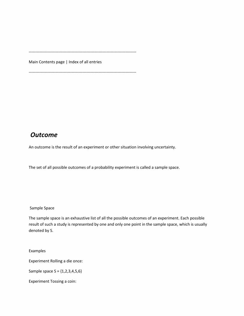
Outcome

An outcome is the result of an experiment or other situation involving uncertainty.

The set of all possible outcomes of a probability experiment is called a sample space.

Sample Space

The sample space is an exhaustive list of all the possible outcomes of an experiment. Each possible

result of such a study is represented by one and only one point in the sample space, which is usually

denoted by S.

Examples

Experiment Rolling a die once:

Sample space S = {1,2,3,4,5,6}

Experiment Tossing a coin:

Sample space S = {Heads,Tails}

Experiment Measuring the height (cms) of a girl on her first day at school:

Sample space S = the set of all possible real numbers

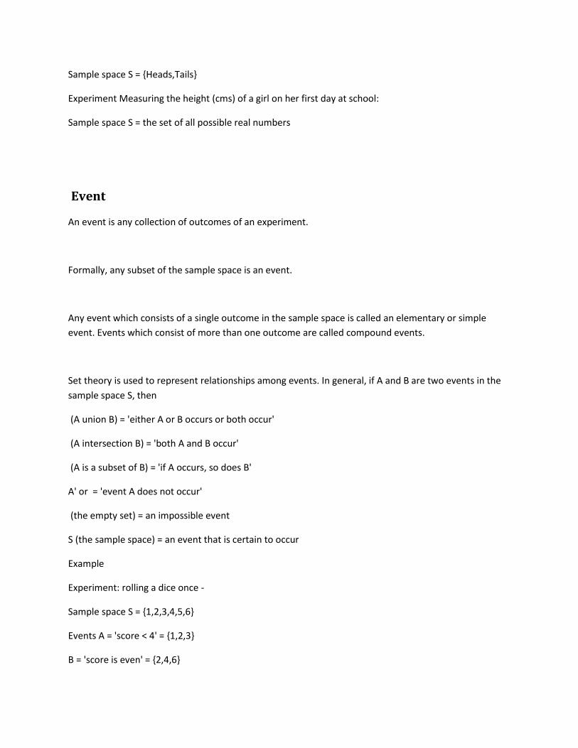
Event

An event is any collection of outcomes of an experiment.

Formally, any subset of the sample space is an event.

Any event which consists of a single outcome in the sample space is called an elementary or simple

event. Events which consist of more than one outcome are called compound events.

Set theory is used to represent relationships among events. In general, if A and B are two events in the

sample space S, then

(A union B) = 'either A or B occurs or both occur'

(A intersection B) = 'both A and B occur'

(A is a subset of B) = 'if A occurs, so does B'

A' or = 'event A does not occur'

(the empty set) = an impossible event

S (the sample space) = an event that is certain to occur

Example

Experiment: rolling a dice once -


Events A = 'score < 4' = {1,2,3}

B = 'score is even' = {2,4,6}

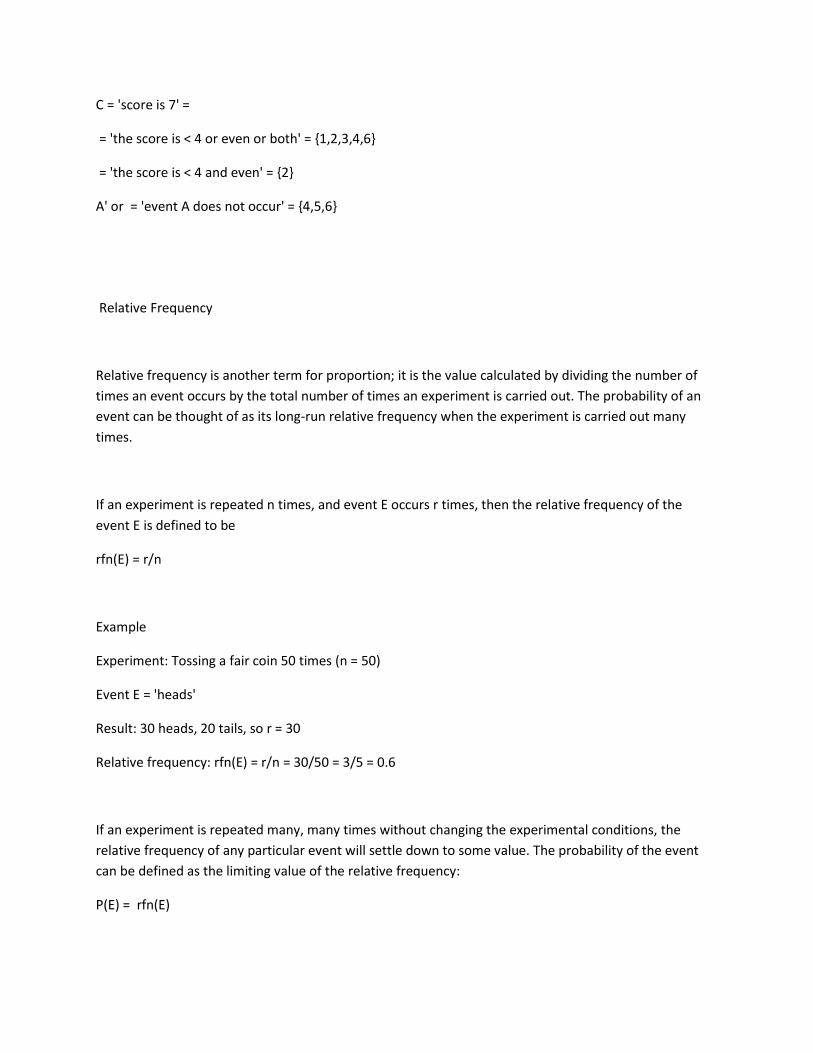
C = 'score is 7' =

= 'the score is < 4 or even or both' = {1,2,3,4,6}

= 'the score is < 4 and even' = {2}

A' or = 'event A does not occur' = {4,5,6}

Relative Frequency

Relative frequency is another term for proportion; it is the value calculated by dividing the number of

times an event occurs by the total number of times an experiment is carried out. The probability of an

event can be thought of as its long-run relative frequency when the experiment is carried out many

times.

If an experiment is repeated n times, and event E occurs r times, then the relative frequency of the

event E is defined to be

rfn(E) = r/n

Example

Experiment: Tossing a fair coin 50 times (n = 50)

Event E = 'heads'

Result: 30 heads, 20 tails, so r = 30

Relative frequency: rfn(E) = r/n = 30/50 = 3/5 = 0.6

If an experiment is repeated many, many times without changing the experimental conditions, the

relative frequency of any particular event will settle down to some value. The probability of the event

can be defined as the limiting value of the relative frequency:

P(E) = rfn(E)

For example, in the above experiment, the relative frequency of the event 'heads' will settle down to a

value of approximately 0.5 if the experiment is repeated many more times.

Probability

A probability provides a quantatative description of the likely occurrence of a particular event.

Probability is conventionally expressed on a scale from 0 to 1; a rare event has a probability close to 0, a

very common event has a probability close to 1.

The probability of an event has been defined as its long-run relative frequency. It has also been thought

of as a personal degree of belief that a particular event will occur (subjective probability).

In some experiments, all outcomes are equally likely. For example if you were to choose one winner in a

raffle from a hat, all raffle ticket holders are equally likely to win, that is, they have the same probability

of their ticket being chosen. This is the equally-likely outcomes model and is defined to be:

P(E) = number of outcomes corresponding to event E

--------------------------------------------------------------------------------

total number of outcomes

Examples

The probability of drawing a spade from a pack of 52 well-shuffled playing cards is 13/52 = 1/4 = 0.25

since

event E = 'a spade is drawn';

the number of outcomes corresponding to E = 13 (spades);

the total number of outcomes = 52 (cards).

When tossing a coin, we assume that the results 'heads' or 'tails' each have equal probabilities of 0.5.

Subjective Probability

A subjective probability describes an individual's personal judgement about how likely a particular event

is to occur. It is not based on any precise computation but is often a reasonable assessment by a

knowledgeable person.

Like all probabilities, a subjective probability is conventionally expressed on a scale from 0 to 1; a rare

event has a subjective probability close to 0, a very common event has a subjective probability close to

1.

A person's subjective probability of an event describes his/her degree of belief in the event.

Example

A Rangers supporter might say, "I believe that Rangers have probability of 0.9 of winning the Scottish

Premier Division this year since they have been playing really well."

Independent Events

Two events are independent if the occurrence of one of the events gives us no information about

whether or not the other event will occur; that is, the events have no influence on each other.

In probability theory we say that two events, A and B, are independent if the probability that they both

occur is equal to the product of the probabilities of the two individual events, i.e.

The idea of independence can be extended to more than two events. For example, A, B and C are

independent if:

A and B are independent; A and C are independent and B and C are independent (pairwise

independence);

If two events are independent then they cannot be mutually exclusive (disjoint) and vice versa.

Example

Suppose that a man and a woman each have a pack of 52 playing cards. Each draws a card from his/her

pack. Find the probability that they each draw the ace of clubs.

We define the events:

A = probability that man draws ace of clubs = 1/52

B = probability that woman draws ace of clubs = 1/52

Clearly events A and B are independent so:

= 1/52 . 1/52 = 0.00037

That is, there is a very small chance that the man and the woman will both draw the ace of clubs.

See also conditional probability.

Mutually Exclusive Events

Two events are mutually exclusive (or disjoint) if it is impossible for them to occur together.

Formally, two events A and B are mutually exclusive if and only if

If two events are mutually exclusive, they cannot be independent and vice versa.

Examples

Experiment: Rolling a die once


Events A = 'observe an odd number' = {1,3,5}

B = 'observe an even number' = {2,4,6}

= the empty set, so A and B are mutually exclusive.

A subject in a study cannot be both male and female, nor can they be aged 20 and 30. A subject could

however be both male and 20, or both female and 30.

Addition Rule

The addition rule is a result used to determine the probability that event A or event B occurs or both

occur.

The result is often written as follows, using set notation:

where:

P(A) = probability that event A occurs

P(B) = probability that event B occurs

= probability that event A or event B occurs

= probability that event A and event B both occur

For mutually exclusive events, that is events which cannot occur together:

= 0

The addition rule therefore reduces to

= P(A) + P(B)

For independent events, that is events which have no influence on each other:

The addition rule therefore reduces to

Example

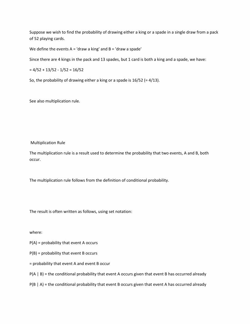
Suppose we wish to find the probability of drawing either a king or a spade in a single draw from a pack

of 52 playing cards.

We define the events A = 'draw a king' and B = 'draw a spade'

Since there are 4 kings in the pack and 13 spades, but 1 card is both a king and a spade, we have:

= 4/52 + 13/52 - 1/52 = 16/52

So, the probability of drawing either a king or a spade is 16/52 (= 4/13).

See also multiplication rule.

Multiplication Rule

The multiplication rule is a result used to determine the probability that two events, A and B, both

occur.

The multiplication rule follows from the definition of conditional probability.


where:



= probability that event A and event B occur

P(A | B) = the conditional probability that event A occurs given that event B has occurred already

P(B | A) = the conditional probability that event B occurs given that event A has occurred already

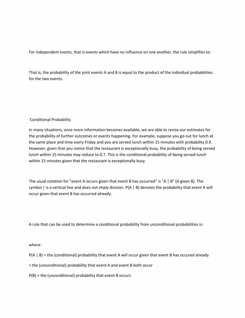
For independent events, that is events which have no influence on one another, the rule simplifies to:

That is, the probability of the joint events A and B is equal to the product of the individual probabilities

for the two events.

Conditional Probability

In many situations, once more information becomes available, we are able to revise our estimates for

the probability of further outcomes or events happening. For example, suppose you go out for lunch at

the same place and time every Friday and you are served lunch within 15 minutes with probability 0.9.

However, given that you notice that the restaurant is exceptionally busy, the probability of being served

lunch within 15 minutes may reduce to 0.7. This is the conditional probability of being served lunch

within 15 minutes given that the restaurant is exceptionally busy.

The usual notation for "event A occurs given that event B has occurred" is "A | B" (A given B). The

symbol | is a vertical line and does not imply division. P(A | B) denotes the probability that event A will

occur given that event B has occurred already.

A rule that can be used to determine a conditional probability from unconditional probabilities is:

where:

P(A | B) = the (conditional) probability that event A will occur given that event B has occured already

= the (unconditional) probability that event A and event B both occur

P(B) = the (unconditional) probability that event B occurs

Law of Total Probability


where:


= probability that event A and event B both occur

= probability that event A and event B' both occur, i.e. A occurs and B does not.

Using the multiplication rule, this can be expressed as

P(A) = P(A | B).P(B) + P(A | B').P(B')

Bayes' Theorem

Bayes' Theorem is a result that allows new information to be used to update the conditional probability

of an event.

Using the multiplication rule, gives Bayes' Theorem in its simplest form:

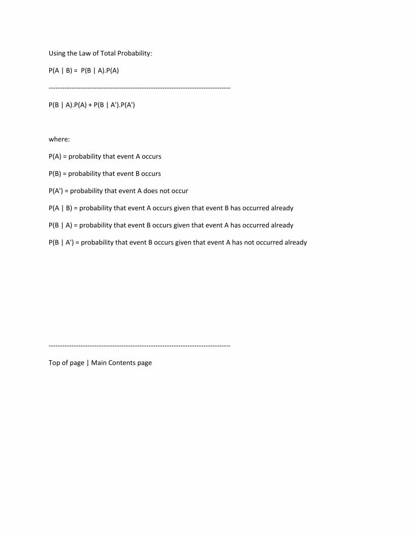
Using the Law of Total Probability:

P(A | B) = P(B | A).P(A)

--------------------------------------------------------------------------------

P(B | A).P(A) + P(B | A').P(A')

where:



P(A') = probability that event A does not occur

P(A | B) = probability that event A occurs given that event B has occurred already

P(B | A) = probability that event B occurs given that event A has occurred already

P(B | A') = probability that event B occurs given that event A has not occurred already

--------------------------------------------------------------------------------

Top of page | Main Contents page