Embed Size (px)
Citation preview
Prof. Pier Luca Lanzi
Classification: Other Methods���Data Mining and Text Mining (UIC 583 @ Politecnico di Milano)
Prof. Pier Luca Lanzi
Study Material
• Mining of Massive Datasets Section 12.3, 12.4• Data Mining and Analysis: Fundamental Concepts and Algorithms
- Chapter 18 & 19
2
Prof. Pier Luca Lanzi
What is Instance-Based Learning?
Prof. Pier Luca Lanzi
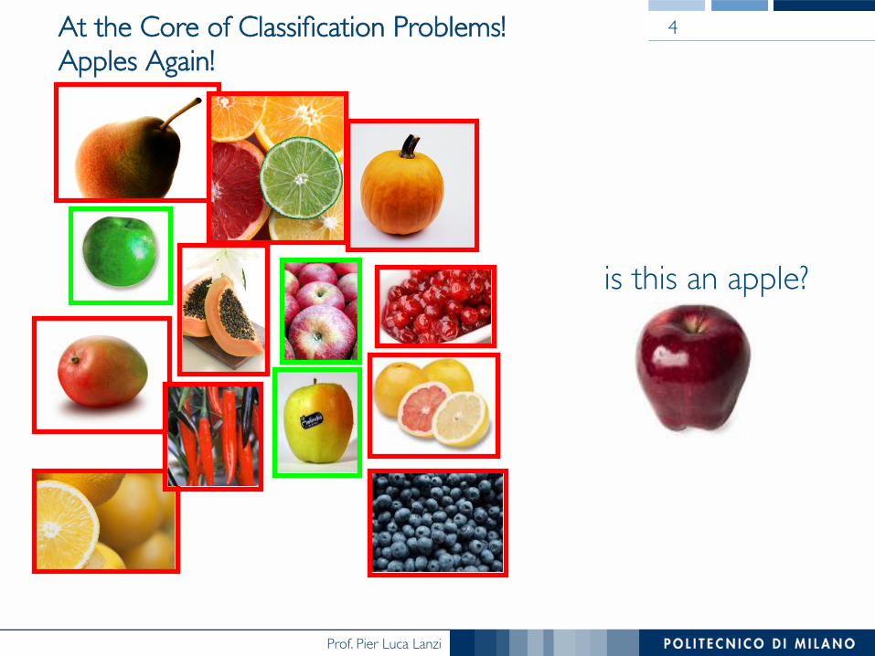
At the Core of Classification Problems!���Apples Again!
4
is this an apple?
Prof. Pier Luca Lanzi
Instance-Based Learning
• To decide the label for an unseen example, consider the k examples from the training data that are more similar to the unknown one
• Classify the unknown example using the most frequent class
5
Prof. Pier Luca Lanzi
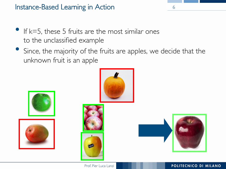
Instance-Based Learning in Action
• If k=5, these 5 fruits are the most similar ones���to the unclassified example
• Since, the majority of the fruits are apples, we decide that the unknown fruit is an apple
6
Prof. Pier Luca Lanzi
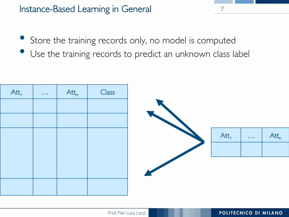
Instance-Based Learning in General
• Store the training records only, no model is computed • Use the training records to predict an unknown class label
7
Att1 … Attn Class
Att1 … Attn
Prof. Pier Luca Lanzi
Instance-Based Methods
• They are the simplest form of learning
• The training dataset is searched for the instances that are more similar to the unlabeled instance
• The training dataset is the model itself, it is the knowledge
• The similarity function defines what’s “learned”
• They implement a “lazy evaluation” (or lazy learning) scheme, nothing happens until a new unlabeled instance must be classified
• Known methods include “Rote Learning”, “Case Base Reasoning”, “k-Nearest Neighbor”
8
Prof. Pier Luca Lanzi
K-Nearest-Neighbor Classifiers
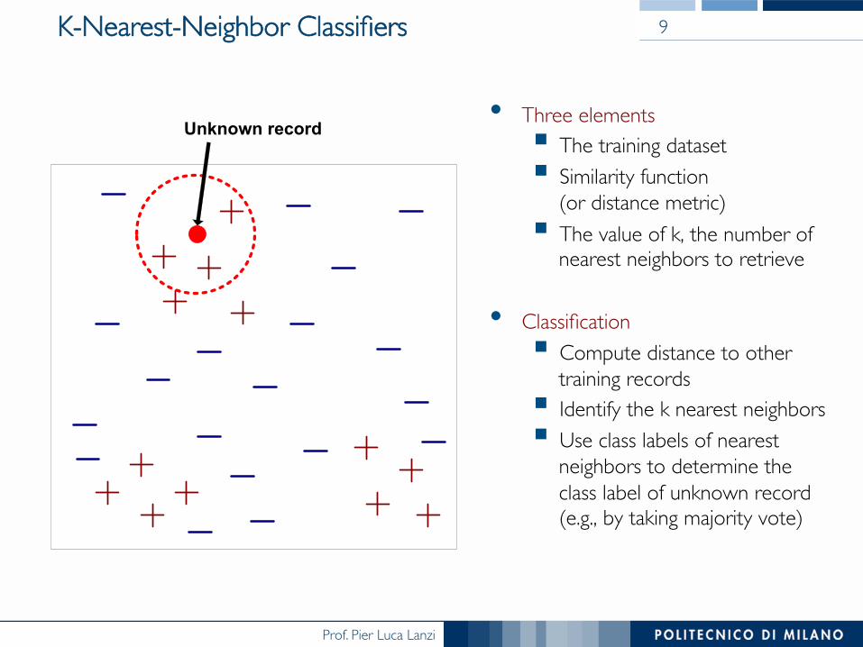
• Three elements§ The training dataset§ Similarity function ���
(or distance metric)§ The value of k, the number of
nearest neighbors to retrieve
• Classification§ Compute distance to other
training records§ Identify the k nearest neighbors § Use class labels of nearest
neighbors to determine the class label of unknown record (e.g., by taking majority vote)
9
Unknown record
Prof. Pier Luca Lanzi
How Many Neighbors? 10
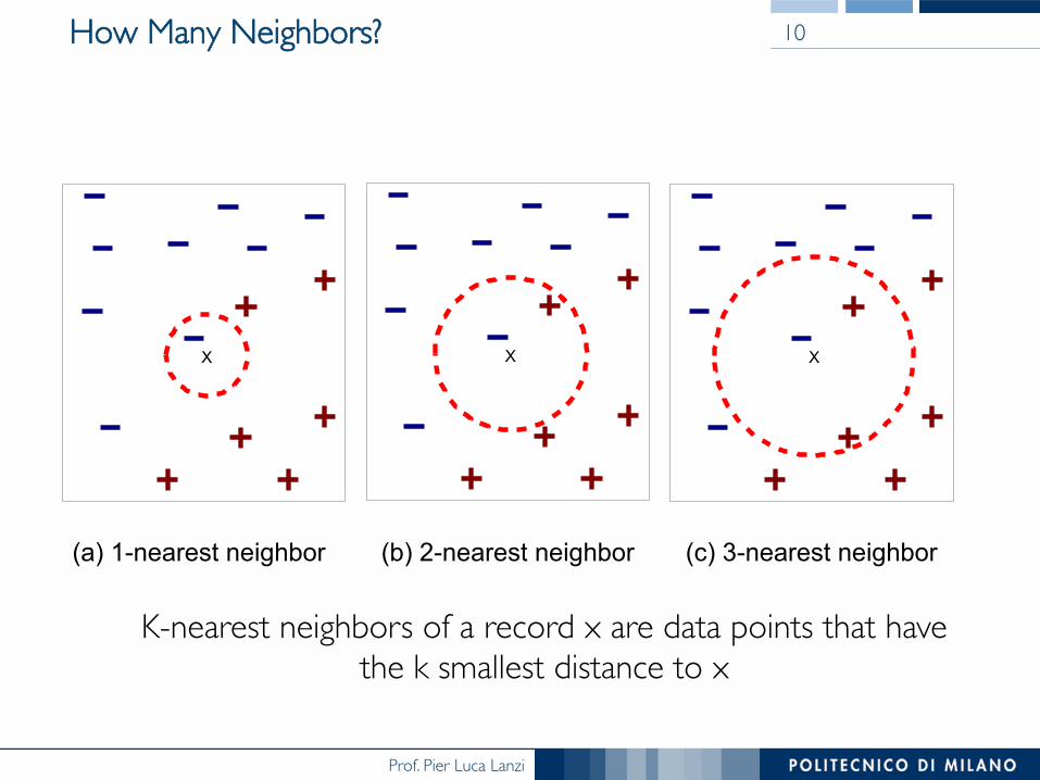
X X X
(a) 1-nearest neighbor (b) 2-nearest neighbor (c) 3-nearest neighbor
K-nearest neighbors of a record x are data points that have the k smallest distance to x
Prof. Pier Luca Lanzi
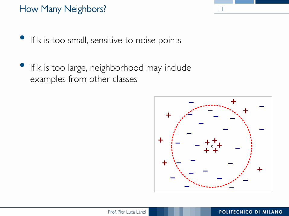
How Many Neighbors?
• If k is too small, sensitive to noise points
• If k is too large, neighborhood may include ���examples from other classes
11
X
Prof. Pier Luca Lanzi
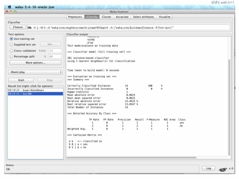
kNN with k=1
Prof. Pier Luca Lanzi
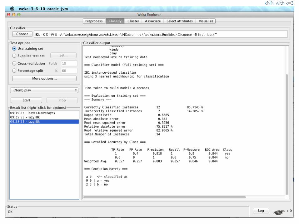
kNN with k=3
Prof. Pier Luca Lanzi
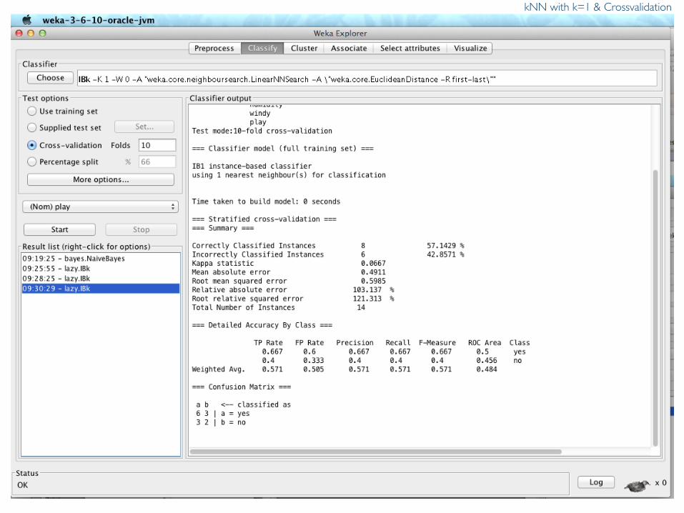
kNN with k=1 & Crossvalidation
Prof. Pier Luca Lanzi
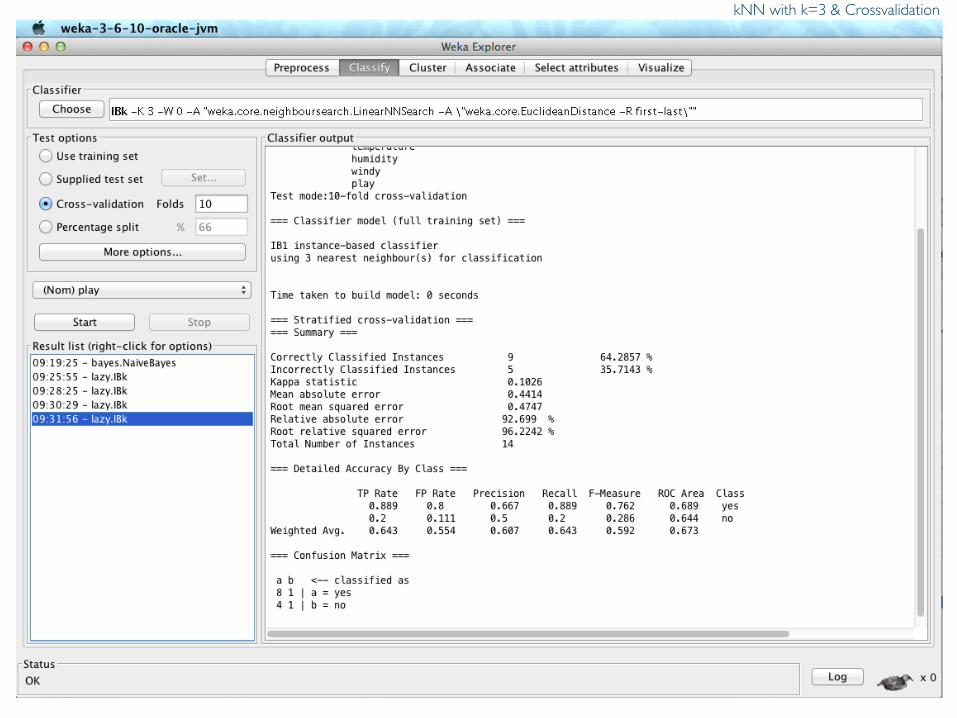
kNN with k=3 & Crossvalidation
Prof. Pier Luca Lanzi
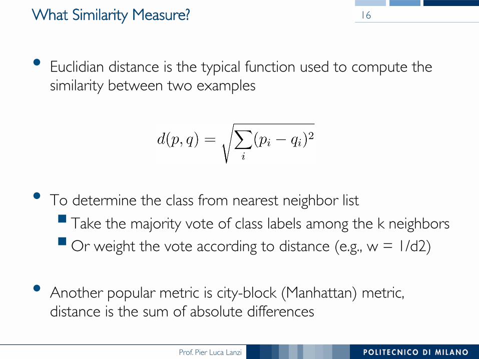
What Similarity Measure?
• Euclidian distance is the typical function used to compute the similarity between two examples
• To determine the class from nearest neighbor list§ Take the majority vote of class labels among the k neighbors§ Or weight the vote according to distance (e.g., w = 1/d2)
• Another popular metric is city-block (Manhattan) metric, ���distance is the sum of absolute differences
16
Prof. Pier Luca Lanzi
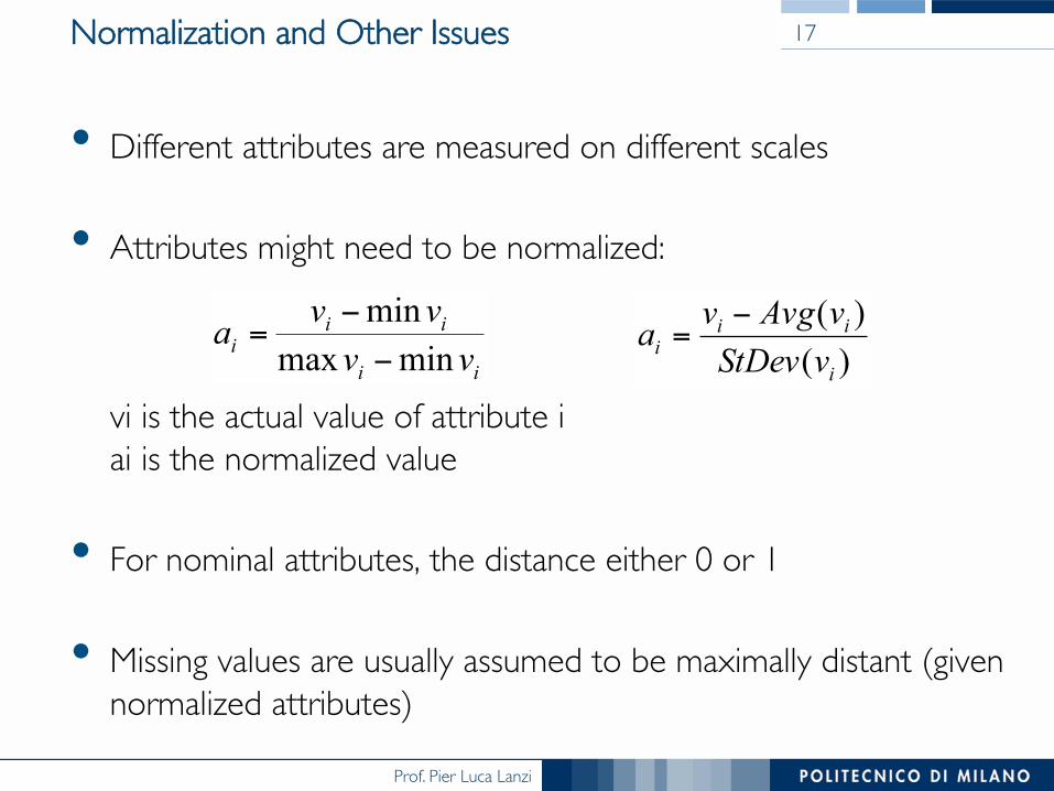
Normalization and Other Issues
• Different attributes are measured on different scales
• Attributes might need to be normalized:������������vi is the actual value of attribute i���ai is the normalized value
• For nominal attributes, the distance either 0 or 1
• Missing values are usually assumed to be maximally distant (given normalized attributes)
17
ii
iii vv
vvaminmax
min−
−=
)()(
i
iii vStDev
vAvgva −=
Prof. Pier Luca Lanzi
Discussion
• K-Nearest Neighbor is often very accurate but slow, since simple version scans entire training data to derive a prediction
• Assumes all attributes are equally important, thus may need attribute selection or weights
• Statisticians have used k-NN since early 1950s,���If n → ∞ and k/n → 0, error approaches minimum
18
Prof. Pier Luca Lanzi
Naïve Bayes
Prof. Pier Luca Lanzi
Bayes Probability
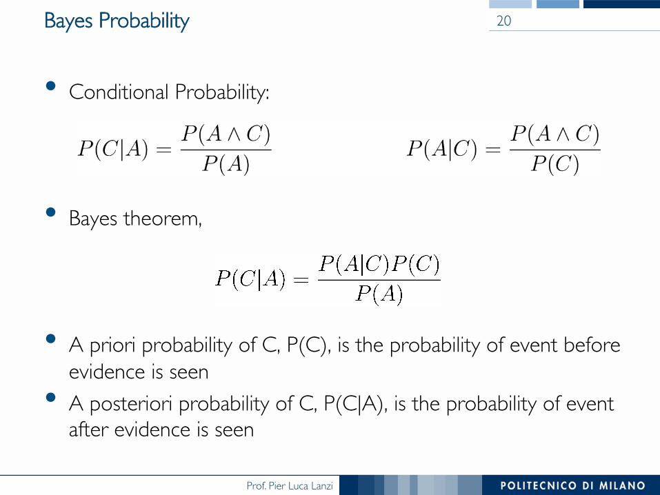
• Conditional Probability:
• Bayes theorem,
• A priori probability of C, P(C), is the probability of event before evidence is seen
• A posteriori probability of C, P(C|A), is the probability of event after evidence is seen
20
Prof. Pier Luca Lanzi
Naïve Bayes Classifiers
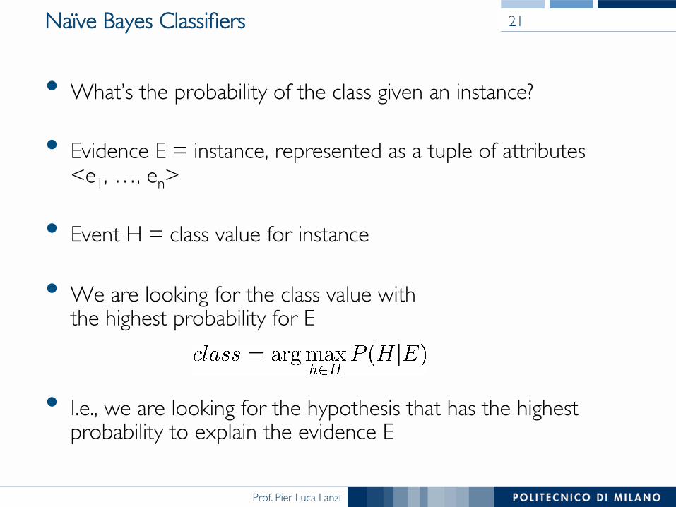
• What’s the probability of the class given an instance?
• Evidence E = instance, represented as a tuple of attributes ���<e1, …, en>
• Event H = class value for instance
• We are looking for the class value with ���the highest probability for E
• I.e., we are looking for the hypothesis that has the highest probability to explain the evidence E
21
Prof. Pier Luca Lanzi
Naïve Bayes Classifiers
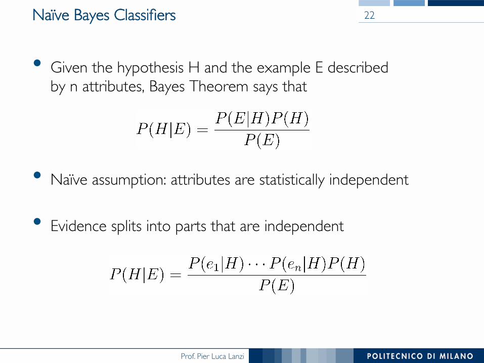
• Given the hypothesis H and the example E described ���by n attributes, Bayes Theorem says that
• Naïve assumption: attributes are statistically independent
• Evidence splits into parts that are independent
22
Prof. Pier Luca Lanzi
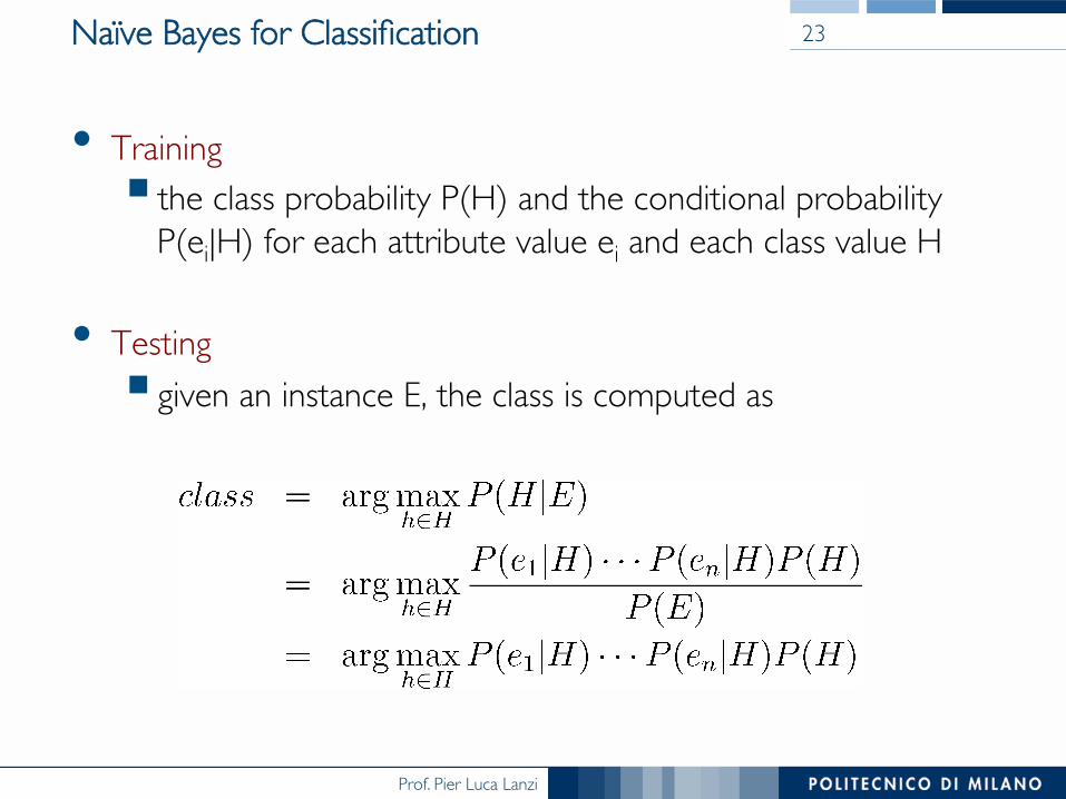
Naïve Bayes for Classification
• Training§ the class probability P(H) and the conditional probability ���
P(ei|H) for each attribute value ei and each class value H
• Testing§ given an instance E, the class is computed as
23
Prof. Pier Luca Lanzi
Naïve Bayes Classifier
• It is the “opposite” of OneRule as it uses all the attributes
• Two assumptions§ Attributes are equally important§ Attribute are statistically independent
• Statistically independent means that knowing the value of one attribute says nothing about the value of another (if the class is known)
• Independence assumption is almost never correct! But the scheme works well in practice
24
Prof. Pier Luca Lanzi
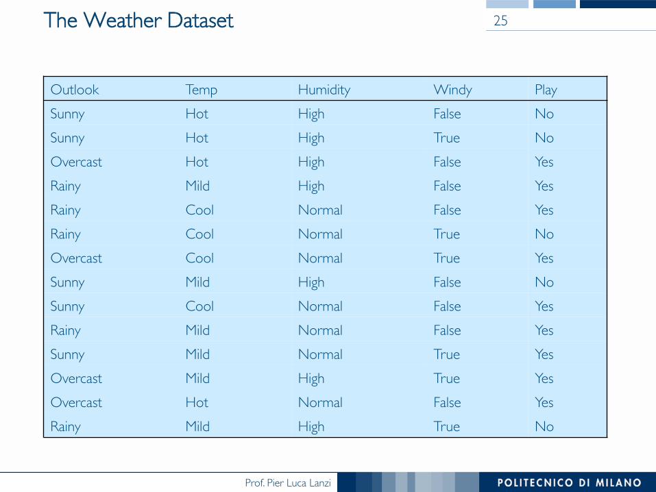
The Weather Dataset
Outlook Temp Humidity Windy PlaySunny Hot High False NoSunny Hot High True NoOvercast Hot High False YesRainy Mild High False YesRainy Cool Normal False YesRainy Cool Normal True NoOvercast Cool Normal True YesSunny Mild High False NoSunny Cool Normal False YesRainy Mild Normal False YesSunny Mild Normal True YesOvercast Mild High True YesOvercast Hot Normal False YesRainy Mild High True No
25
Prof. Pier Luca Lanzi
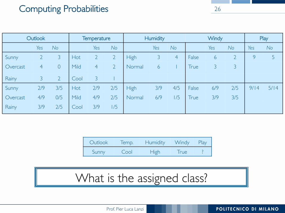
Computing Probabilities 26
Outlook Temperature Humidity Windy PlayYes No Yes No Yes No Yes No Yes No
Sunny 2 3 Hot 2 2 High 3 4 False 6 2 9 5Overcast 4 0 Mild 4 2 Normal 6 1 True 3 3
Rainy 3 2 Cool 3 1Sunny 2/9 3/5 Hot 2/9 2/5 High 3/9 4/5 False 6/9 2/5 9/14 5/14Overcast 4/9 0/5 Mild 4/9 2/5 Normal 6/9 1/5 True 3/9 3/5Rainy 3/9 2/5 Cool 3/9 1/5
Outlook Temp. Humidity Windy PlaySunny Cool High True ?
What is the assigned class?
Prof. Pier Luca Lanzi
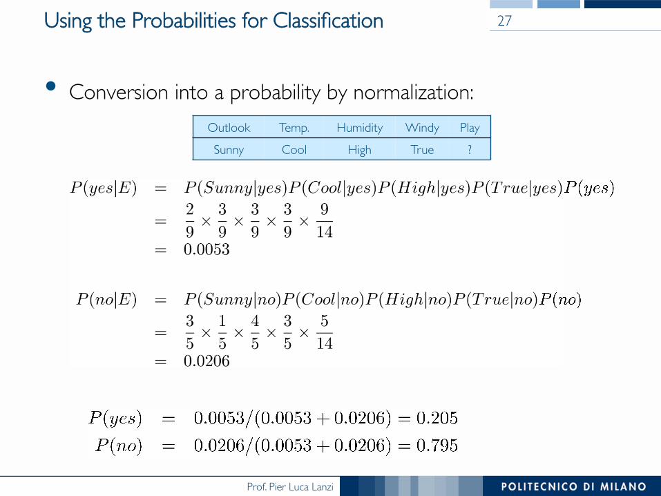
Using the Probabilities for Classification
• Conversion into a probability by normalization:
27
Outlook Temp. Humidity Windy PlaySunny Cool High True ?

Prof. Pier Luca Lanzi
Prof. Pier Luca Lanzi
Prof. Pier Luca Lanzi
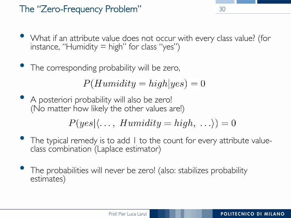
The “Zero-Frequency Problem”
• What if an attribute value does not occur with every class value? (for instance, “Humidity = high” for class “yes”)
• The corresponding probability will be zero,
• A posteriori probability will also be zero!���(No matter how likely the other values are!)
• The typical remedy is to add 1 to the count for every attribute value-class combination (Laplace estimator)
• The probabilities will never be zero! (also: stabilizes probability estimates)
30
Prof. Pier Luca Lanzi
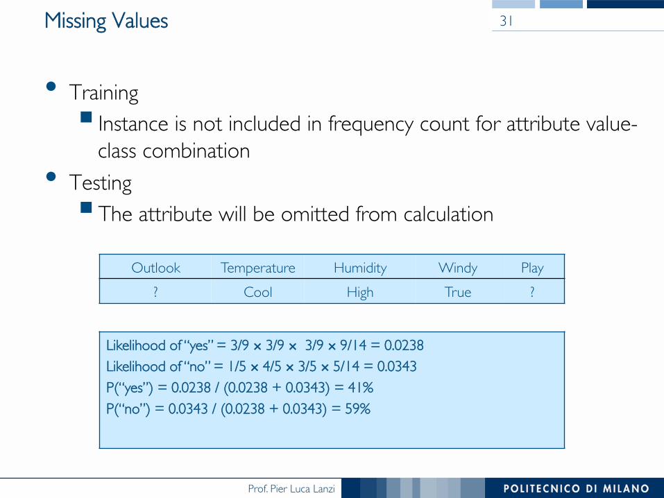
Missing Values
• Training§ Instance is not included in frequency count for attribute value-
class combination• Testing§ The attribute will be omitted from calculation
31
Outlook Temperature Humidity Windy Play? Cool High True ?
Likelihood of “yes” = 3/9 × 3/9 × 3/9 × 9/14 = 0.0238Likelihood of “no” = 1/5 × 4/5 × 3/5 × 5/14 = 0.0343P(“yes”) = 0.0238 / (0.0238 + 0.0343) = 41%P(“no”) = 0.0343 / (0.0238 + 0.0343) = 59%
Prof. Pier Luca Lanzi
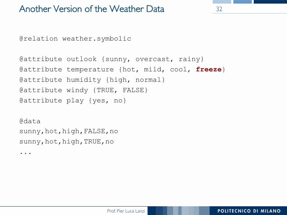
Another Version of the Weather Data
@relation weather.symbolic
@attribute outlook {sunny, overcast, rainy}
@attribute temperature {hot, mild, cool, freeze} @attribute humidity {high, normal}
@attribute windy {TRUE, FALSE}
@attribute play {yes, no}
@data sunny,hot,high,FALSE,no
sunny,hot,high,TRUE,no
...
32
Prof. Pier Luca Lanzi
Prof. Pier Luca Lanzi
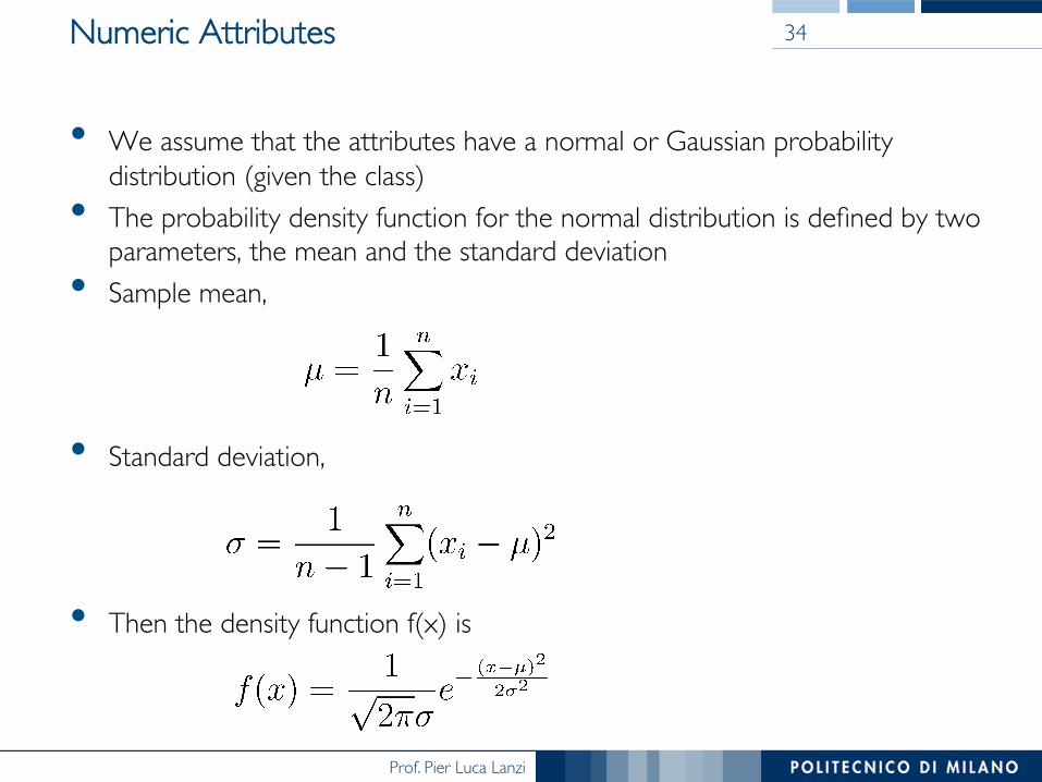
Numeric Attributes
• We assume that the attributes have a normal or Gaussian probability distribution (given the class)
• The probability density function for the normal distribution is defined by two parameters, the mean and the standard deviation
• Sample mean,
• Standard deviation,
• Then the density function f(x) is
34
Prof. Pier Luca Lanzi
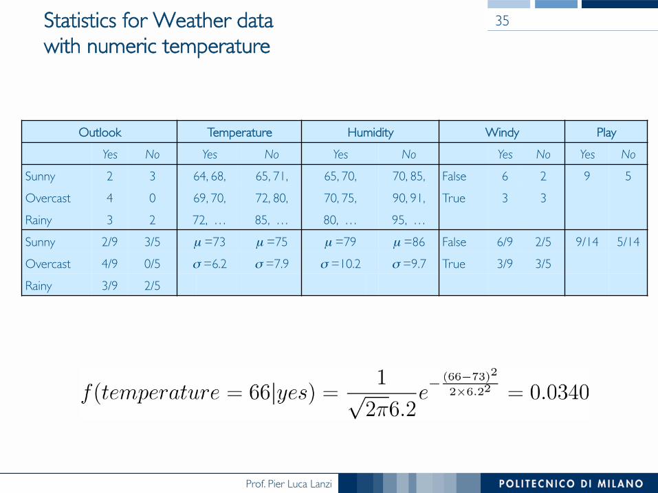
Statistics for Weather data���with numeric temperature
35
Outlook Temperature Humidity Windy PlayYes No Yes No Yes No Yes No Yes No
Sunny 2 3 64, 68, 65, 71, 65, 70, 70, 85, False 6 2 9 5Overcast 4 0 69, 70, 72, 80, 70, 75, 90, 91, True 3 3Rainy 3 2 72, … 85, … 80, … 95, …Sunny 2/9 3/5 µ =73 µ =75 µ =79 µ =86 False 6/9 2/5 9/14 5/14Overcast 4/9 0/5 σ =6.2 σ =7.9 σ =10.2 σ =9.7 True 3/9 3/5Rainy 3/9 2/5
Prof. Pier Luca Lanzi
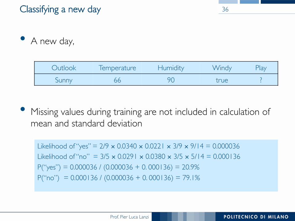
Classifying a new day
• A new day,
• Missing values during training are not included in calculation of mean and standard deviation
36
Outlook Temperature Humidity Windy PlaySunny 66 90 true ?
Likelihood of “yes” = 2/9 × 0.0340 × 0.0221 × 3/9 × 9/14 = 0.000036Likelihood of “no” = 3/5 × 0.0291 × 0.0380 × 3/5 × 5/14 = 0.000136P(“yes”) = 0.000036 / (0.000036 + 0. 000136) = 20.9%P(“no”) = 0.000136 / (0.000036 + 0. 000136) = 79.1%

Prof. Pier Luca Lanzi
Prof. Pier Luca Lanzi
Prof. Pier Luca Lanzi
Discussion
• Naïve Bayes works surprisingly well, even if independence assumption is clearly violated
• Why? Because classification doesn’t require accurate probability estimates as long as maximum probability is assigned to correct class
• However, adding too many redundant attributes will cause problems (e.g. identical attributes)
• Also, many numeric attributes are not normally distributed
39
Prof. Pier Luca Lanzi
Logistic Regression
Prof. Pier Luca Lanzi
Logistic Regression
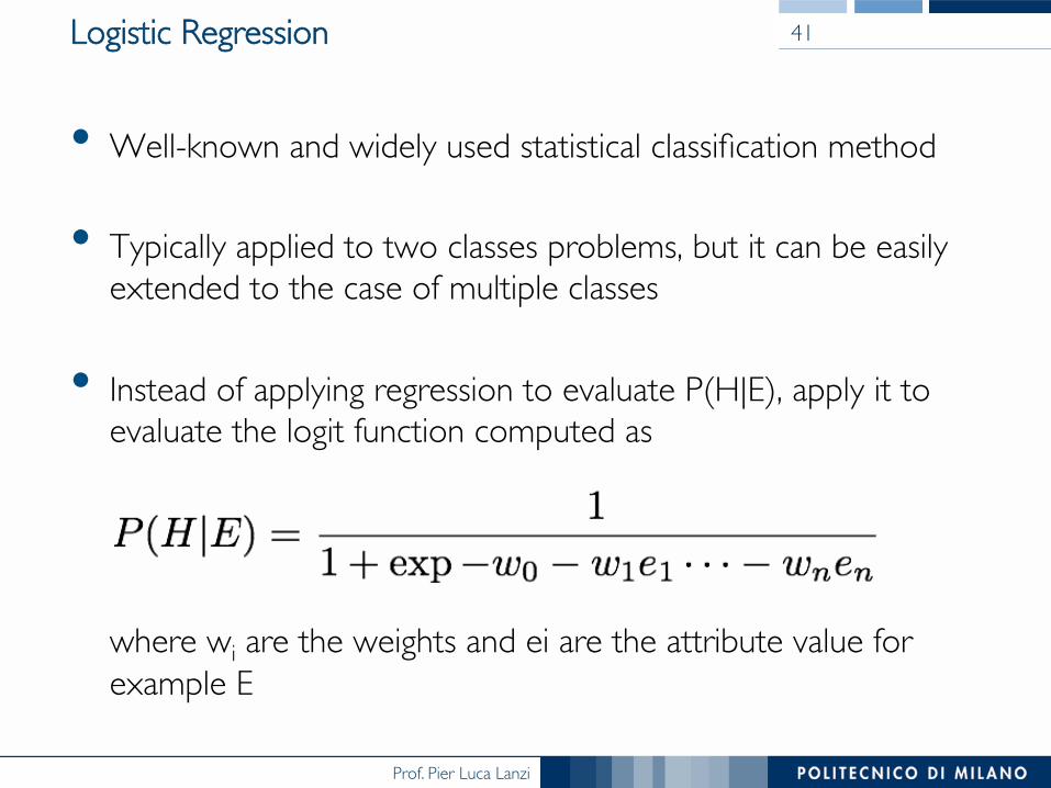
• Well-known and widely used statistical classification method
• Typically applied to two classes problems, but it can be easily extended to the case of multiple classes
• Instead of applying regression to evaluate P(H|E), apply it to evaluate the logit function computed as ���������������where wi are the weights and ei are the attribute value for example E
41
Prof. Pier Luca Lanzi
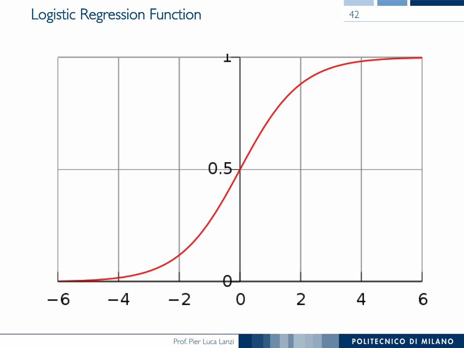
Logistic Regression Function 42
Prof. Pier Luca Lanzi
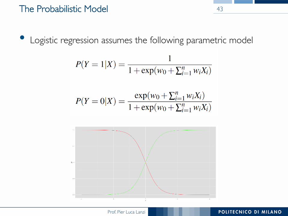
The Probabilistic Model
• Logistic regression assumes the following parametric model
43
Prof. Pier Luca Lanzi
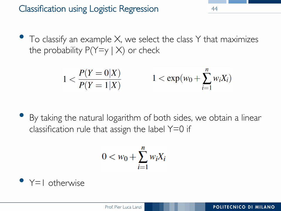
Classification using Logistic Regression
• To classify an example X, we select the class Y that maximizes the probability P(Y=y | X) or check
or
• By taking the natural logarithm of both sides, we obtain a linear classification rule that assign the label Y=0 if
• Y=1 otherwise
44
Prof. Pier Luca Lanzi
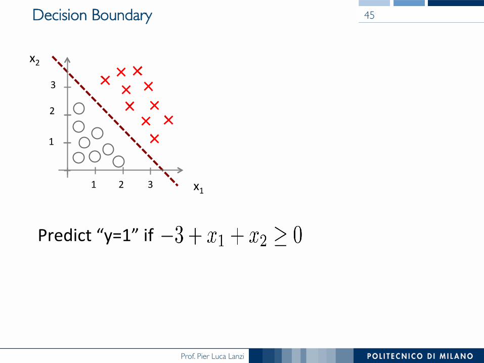
Decision Boundary 45
Predict “y=1” if
x1
x2
1 2 3
1
2
3
Prof. Pier Luca Lanzi
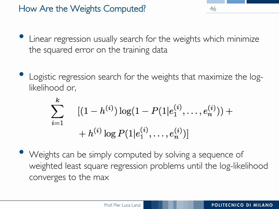
How Are the Weights Computed?
• Linear regression usually search for the weights which minimize the squared error on the training data
• Logistic regression search for the weights that maximize the log-likelihood or,
• Weights can be simply computed by solving a sequence of weighted least square regression problems until the log-likelihood converges to the max
46
Prof. Pier Luca Lanzi
Prof. Pier Luca Lanzi
Prof. Pier Luca Lanzi
Bayesian Belief Networks
Prof. Pier Luca Lanzi
Bayesian Belief Networks
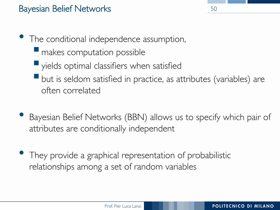
• The conditional independence assumption, § makes computation possible§ yields optimal classifiers when satisfied§ but is seldom satisfied in practice, as attributes (variables) are
often correlated
• Bayesian Belief Networks (BBN) allows us to specify which pair of attributes are conditionally independent
• They provide a graphical representation of probabilistic relationships among a set of random variables
50
Prof. Pier Luca Lanzi
Bayesian Belief Networks
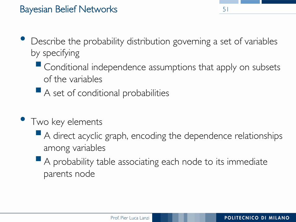
• Describe the probability distribution governing a set of variables by specifying § Conditional independence assumptions that apply on subsets
of the variables§ A set of conditional probabilities
• Two key elements§ A direct acyclic graph, encoding the dependence relationships
among variables§ A probability table associating each node to its immediate
parents node
51
Prof. Pier Luca Lanzi
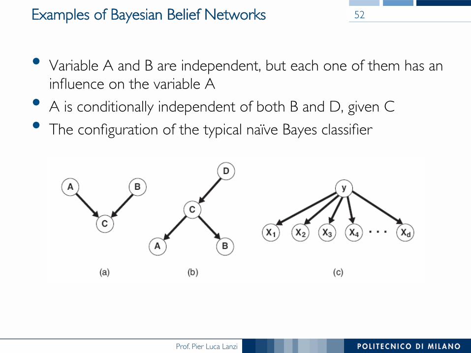
• Variable A and B are independent, but each one of them has an influence on the variable A
• A is conditionally independent of both B and D, given C• The configuration of the typical naïve Bayes classifier
Examples of Bayesian Belief Networks 52
Prof. Pier Luca Lanzi
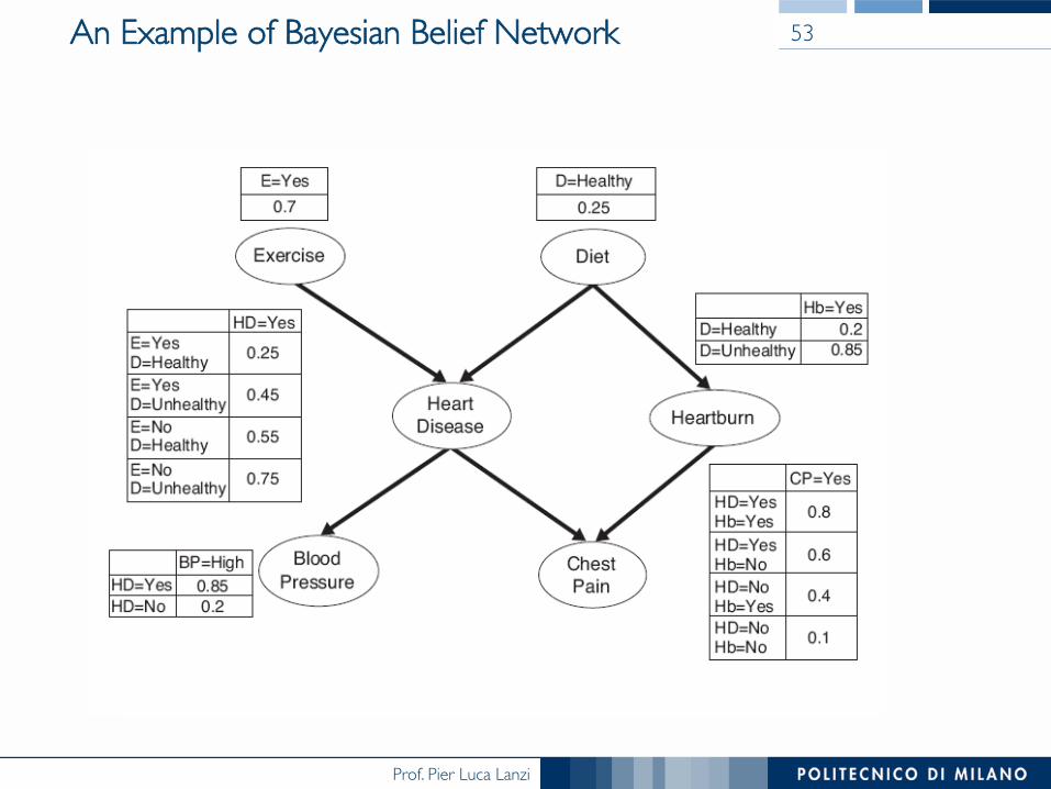
An Example of Bayesian Belief Network 53
Prof. Pier Luca Lanzi
Probability Tables
• The network topology imposes conditions regarding the variable conditional independence
• Each node is associated with a probability table§ If a node X does not have any parents, then ���
the table contains only the prior probability P(X)§ If a node X has only one any parent Y, then ���
the table contains only the conditional probability P(X|Y)§ If a node X has multiple parents, Y1, …, Yk the���
the table contains the conditional probability P(X|Y1…Yk)
54
Prof. Pier Luca Lanzi
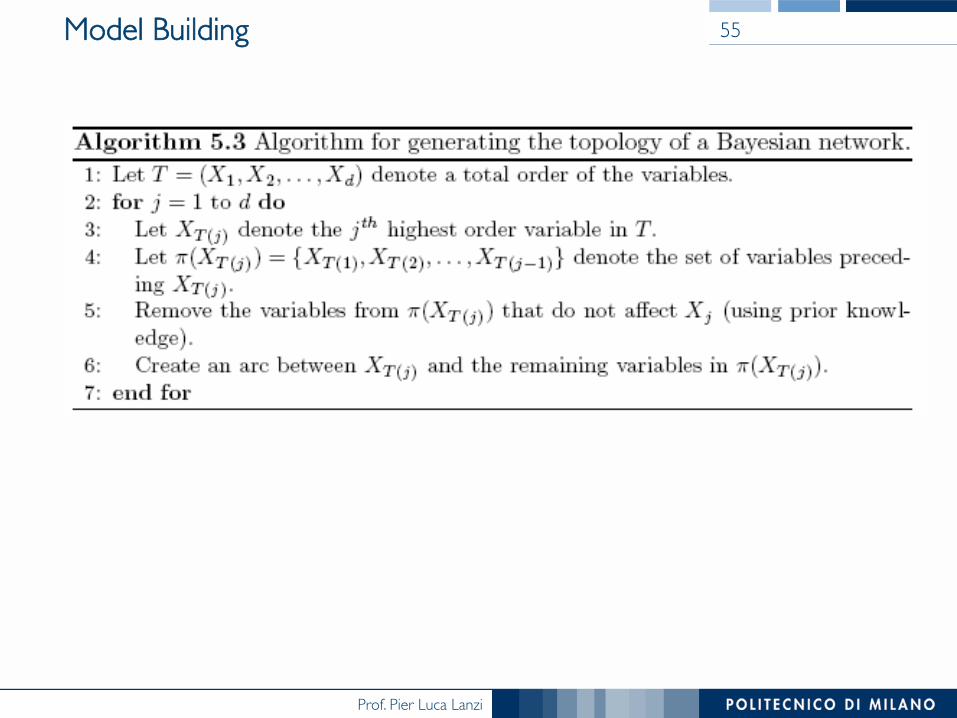
Model Building 55
Prof. Pier Luca Lanzi
Bayesian Belief Networks
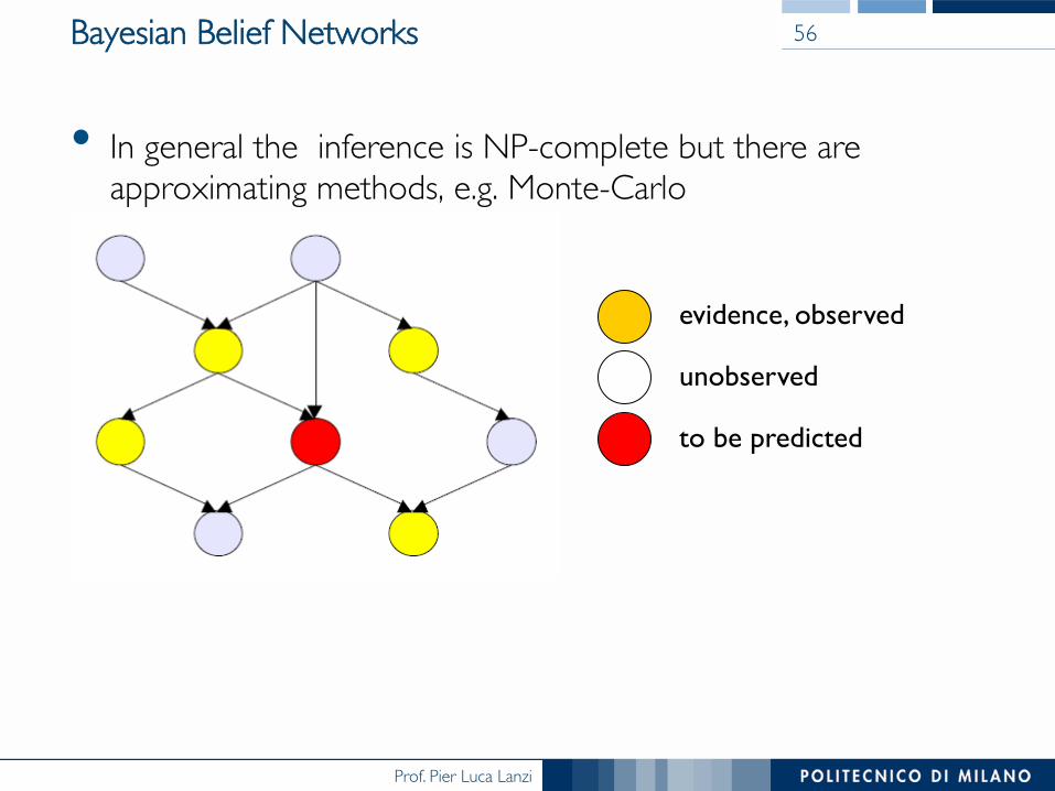
• In general the inference is NP-complete but there are approximating methods, e.g. Monte-Carlo
56
evidence, observed
unobserved
to be predicted

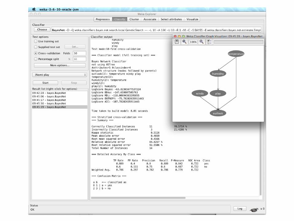
Prof. Pier Luca Lanzihttp://www.cs.waikato.ac.nz/~remco/weka.bn.pdf
Prof. Pier Luca Lanzi
Prof. Pier Luca Lanzi
Bayesian Belief Networks
• Bayesian belief network allows a subset of the variables conditionally independent
• A graphical model of causal relationships• Several cases of learning Bayesian belief networks§ Given both network structure and ���
all the variables is easy§ Given network structure but only some variables§ When the network structure is not known in advance
59
Prof. Pier Luca Lanzi
Bayesian Belief Networks
• BBN provides an approach for capturing prior knowledge of a particular domain using a graphical model
• Building the network is time consuming, but ���adding variables to a network is straightforward
• They can encode causal dependencies among variables• They are well suited to dealing with incomplete data• They are robust to overfitting
60

Prof. Pier Luca Lanzi
Support Vector Machines
Prof. Pier Luca Lanzi
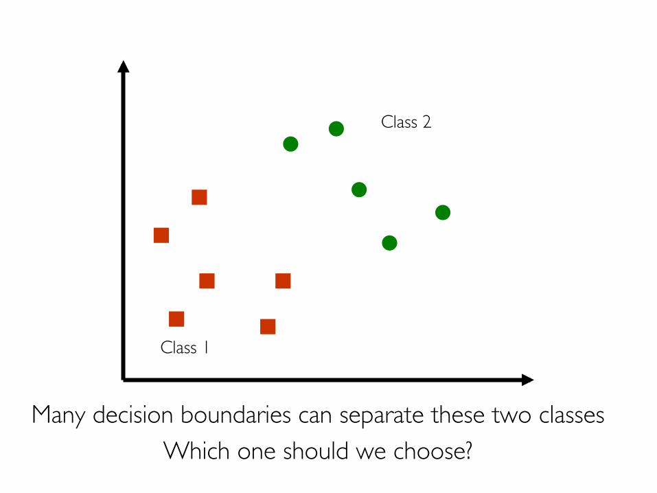
Many decision boundaries can separate these two classesWhich one should we choose?
Class 1
Class 2
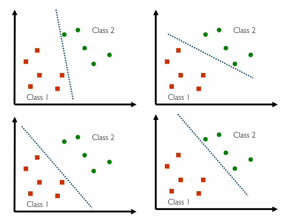
Prof. Pier Luca Lanzi
Class 1
Class 2
Class 1
Class 2
Class 1
Class 2
Class 1
Class 2
Prof. Pier Luca Lanzi
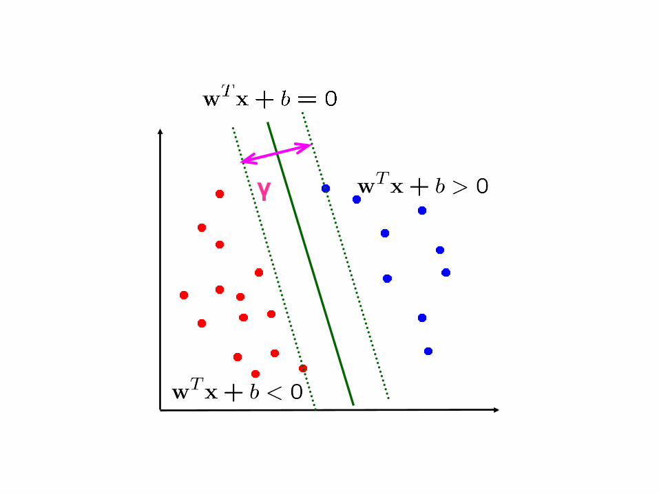
γ
Prof. Pier Luca Lanzi
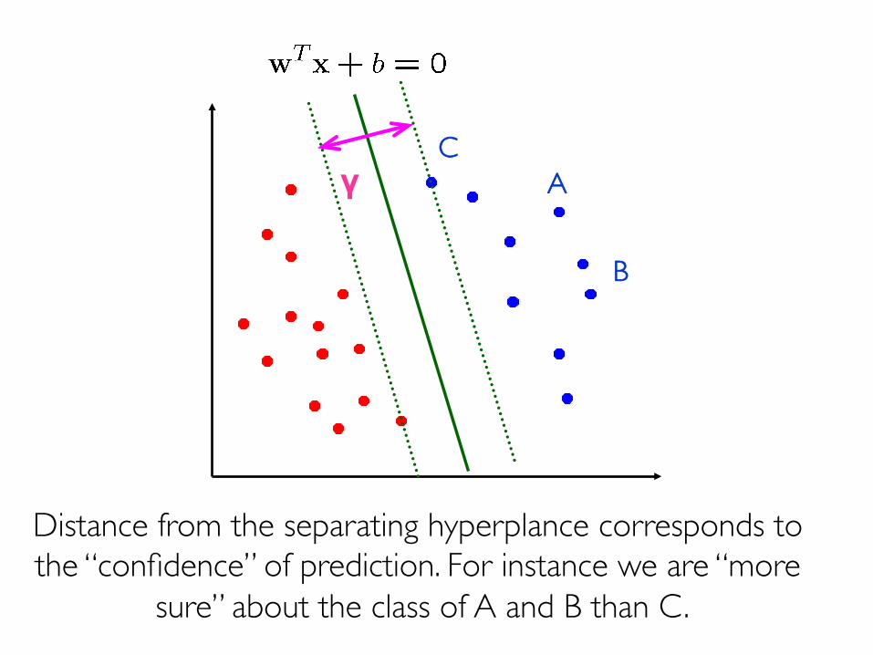
γ AC
B
Distance from the separating hyperplance corresponds to the “confidence” of prediction. For instance we are “more
sure” about the class of A and B than C.
Prof. Pier Luca Lanzi
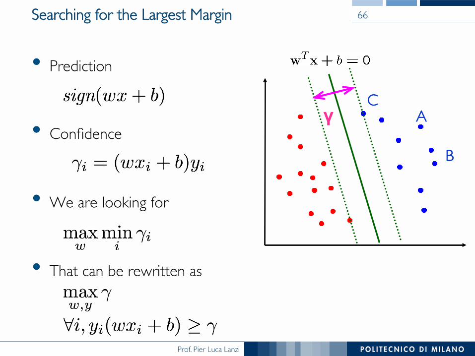
Searching for the Largest Margin
• Prediction
• Confidence
• We are looking for
• That can be rewritten as
66
γ AC
B
Prof. Pier Luca Lanzi
γ AC
B
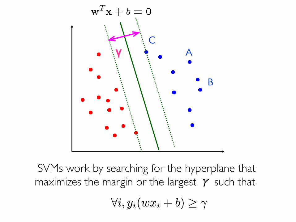
SVMs work by searching for the hyperplane that maximizes the margin or the largest γ such that
Prof. Pier Luca Lanzi
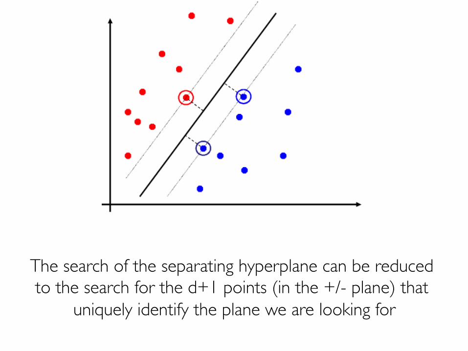
The search of the separating hyperplane can be reduced to the search for the d+1 points (in the +/- plane) that
uniquely identify the plane we are looking for
Prof. Pier Luca Lanzi
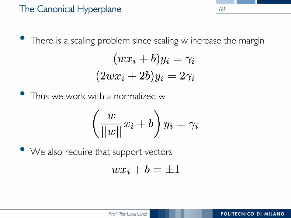
• There is a scaling problem since scaling w increase the margin
• Thus we work with a normalized w
• We also require that support vectors
The Canonical Hyperplane 69
Prof. Pier Luca Lanzi
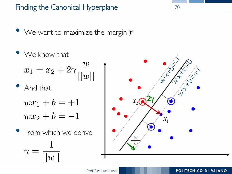
Finding the Canonical Hyperplane
• We want to maximize the marginγ
• We know that
• And that
• From which we derive
70
2γ 2x
1x
|||| ww
Prof. Pier Luca Lanzi
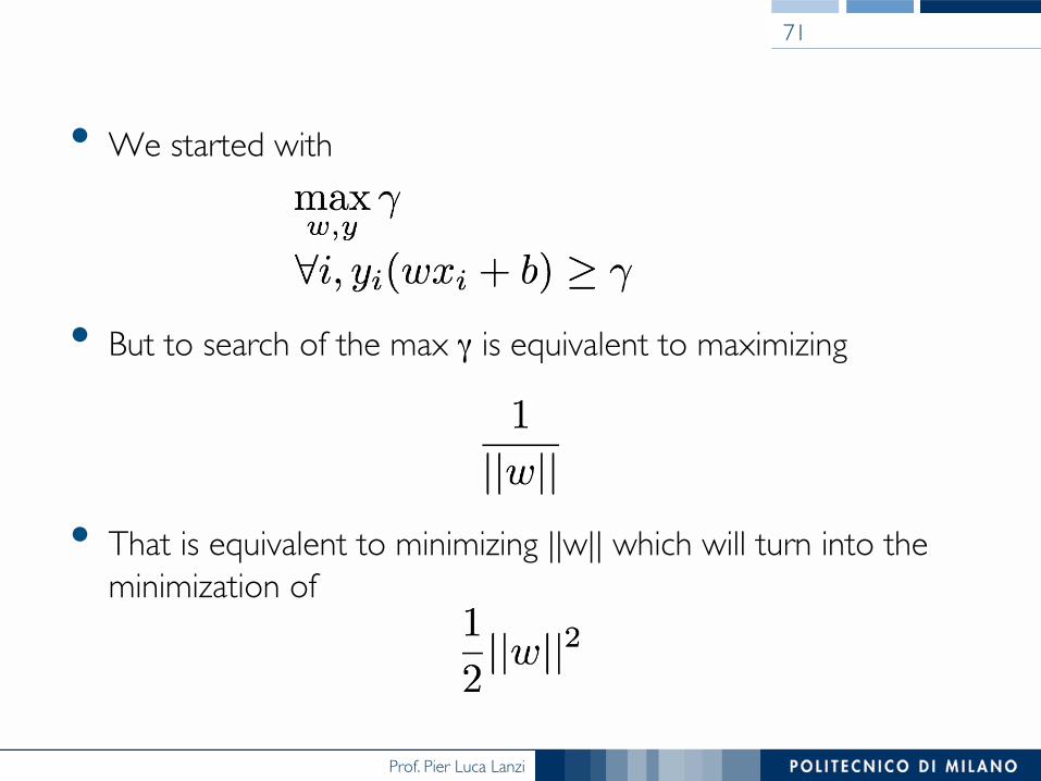
• We started with
• But to search of the max γ is equivalent to maximizing
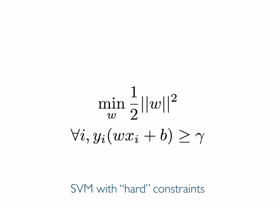
• That is equivalent to minimizing ||w|| which will turn into the minimization of
71
Prof. Pier Luca Lanzi
SVM with “hard” constraints

Prof. Pier Luca Lanzi
Soft-Margin SVMs
Prof. Pier Luca Lanzi
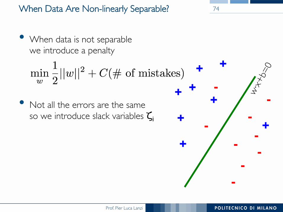
When Data Are Non-linearly Separable?
• When data is not separable���we introduce a penalty
• Not all the errors are the same ���so we introduce slack variables ζi
74
+ +
+ +
+
+
+ -
- -
-
- - -
+ -
-
Prof. Pier Luca Lanzi
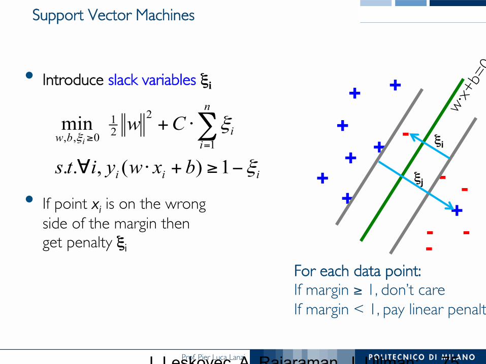
Support Vector Machines
• Introduce slack variables ξi
• If point xi is on the wrong ���side of the margin then ���get penalty ξi
J. Leskovec, A. Rajaraman, J. Ullman: Mining of Massive Datasets, http://www.mmds.org
75
iii
n
iibw
bxwyits
Cwi
ξ
ξξ
−≥+⋅∀
⋅+ ∑=
≥
1)(,..
min1
221
0,,
+ +
+ +
+
+ + - -
- - -
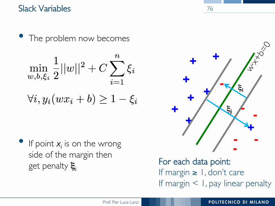
For each data point:If margin ≥ 1, don’t careIf margin < 1, pay linear penalty
+ ξj
- ξi
Prof. Pier Luca Lanzi
Slack Variables
• The problem now becomes
• If point xi is on the wrong ���side of the margin then ���get penalty ξi
76
+ +
+ +
+
+ + - -
- - -
For each data point:If margin ≥ 1, don’t careIf margin < 1, pay linear penalty
+ ξj
- ξi
Prof. Pier Luca Lanzi
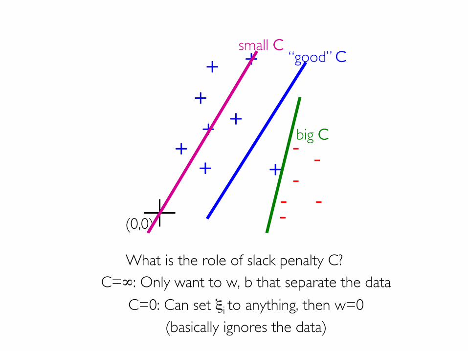
What is the role of slack penalty C?C=∞: Only want to w, b that separate the data
C=0: Can set ξi to anything, then w=0(basically ignores the data)
+ +
++
+
++ - -
---
+ -
big C
“good” Csmall C
(0,0)
Prof. Pier Luca Lanzi
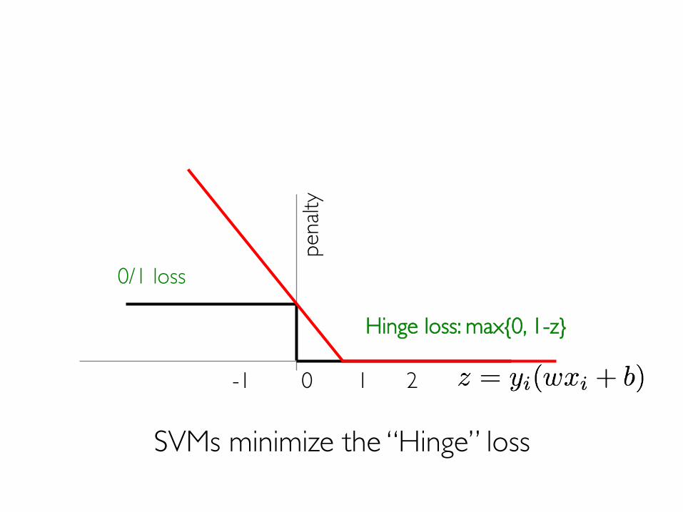
-1 0 1 2
0/1 losspe
nalty
Hinge loss: max{0, 1-z}
SVMs minimize the “Hinge” loss
Prof. Pier Luca Lanzi
How to Estimate w?
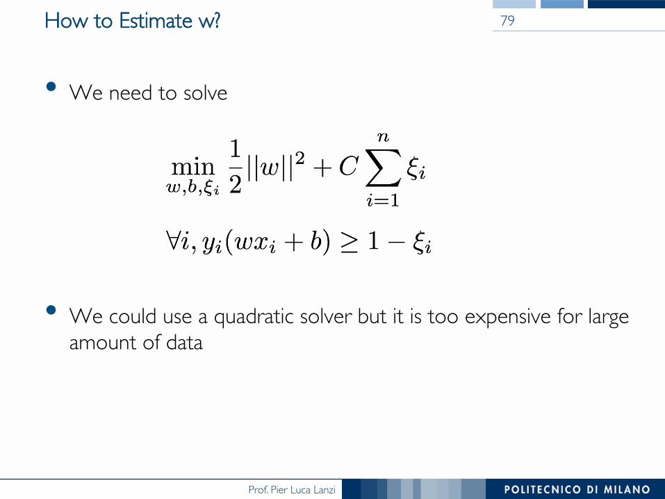
• We need to solve
• We could use a quadratic solver but it is too expensive for large amount of data
79
Prof. Pier Luca Lanzi
Alternative Approach
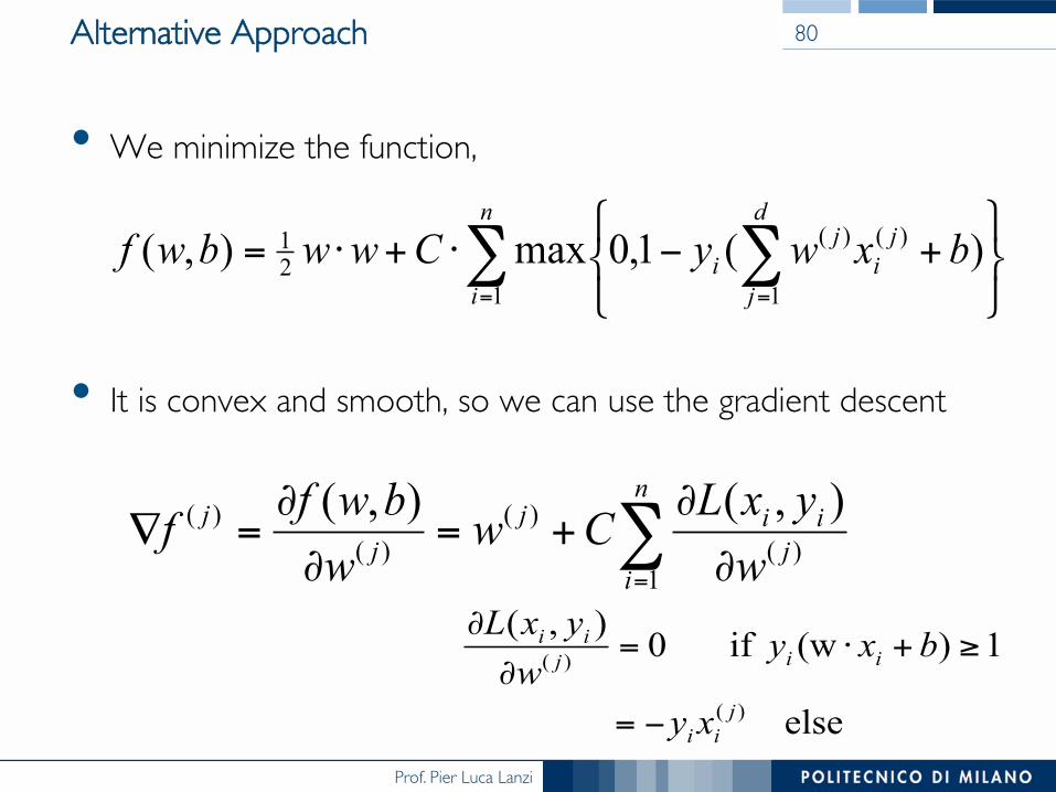
• We minimize the function,
• It is convex and smooth, so we can use the gradient descent
80
∑ ∑= = ⎭
⎬⎫
⎩⎨⎧
+−⋅+⋅=n
i
d
j
ji
ji bxwyCwwbwf
1 1
)()(21 )(1,0max),(
∑= ∂
∂+=
∂
∂=∇
n
ijiij
jj
wyxLCw
wbwff
1)(
)()(
)( ),(),(
else
1)(w if 0),(
)(
)(
jii
iijii
xy
bxywyxL
−=
≥+⋅=∂
∂
Prof. Pier Luca Lanzi
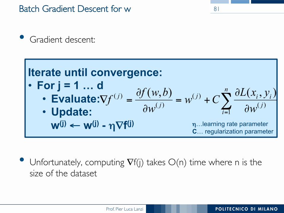
• Gradient descent:
• Unfortunately, computing ∇f(j) takes O(n) time where n is the size of the dataset
Iterate until convergence: • For j = 1 … d
• Evaluate: • Update:
w(j) ← w(j) - η∇f(j)
Batch Gradient Descent for w 81
∑= ∂
∂+=
∂
∂=∇
n
ijiij
jj
wyxLCw
wbwff
1)(
)()(
)( ),(),(
η…learning rate parameter C… regularization parameter
Prof. Pier Luca Lanzi
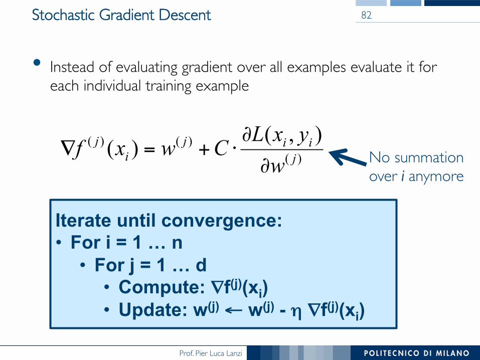
Stochastic Gradient Descent
• Instead of evaluating gradient over all examples evaluate it for each individual training example
82
)()()( ),()( j
iiji
j
wyxLCwxf
∂
∂⋅+=∇
Iterate until convergence: • For i = 1 … n
• For j = 1 … d • Compute: ∇f(j)(xi) • Update: w(j) ← w(j) - η ∇f(j)(xi)
No summation ���over i anymore

Prof. Pier Luca Lanzi
The Kernel Trick
Prof. Pier Luca Lanzi
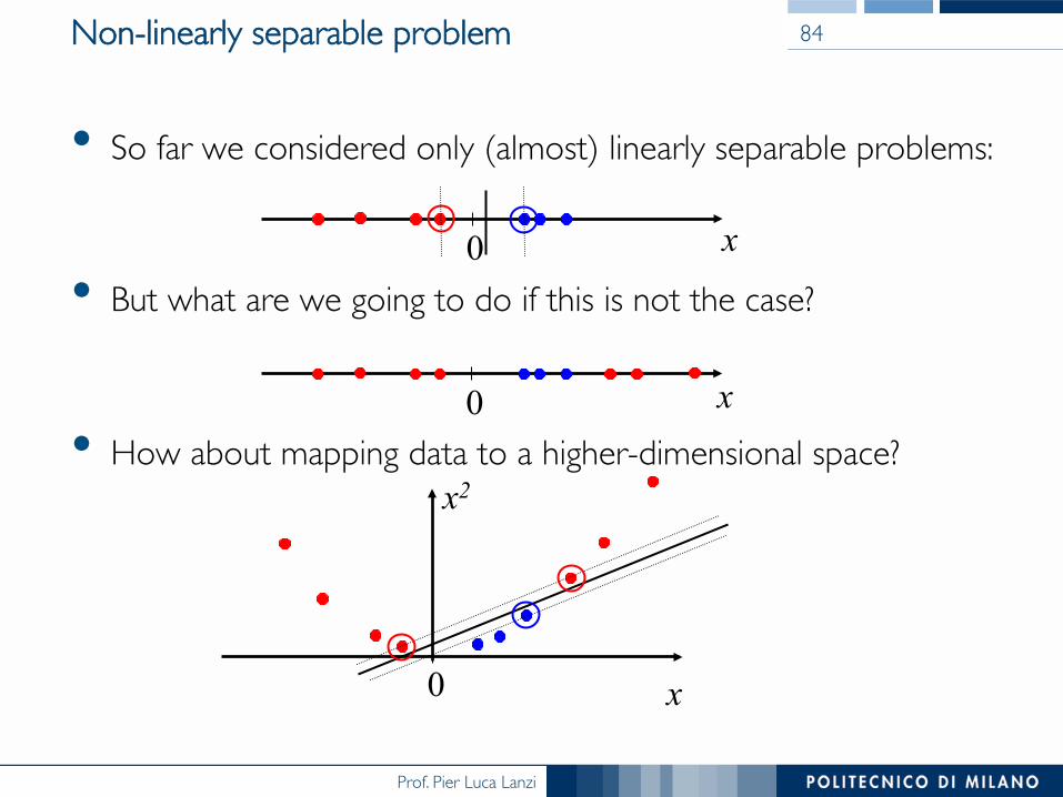
• So far we considered only (almost) linearly separable problems:
• But what are we going to do if this is not the case?
• How about mapping data to a higher-dimensional space?
0 x
0 x
0 x
x2
Non-linearly separable problem 84
Prof. Pier Luca Lanzi
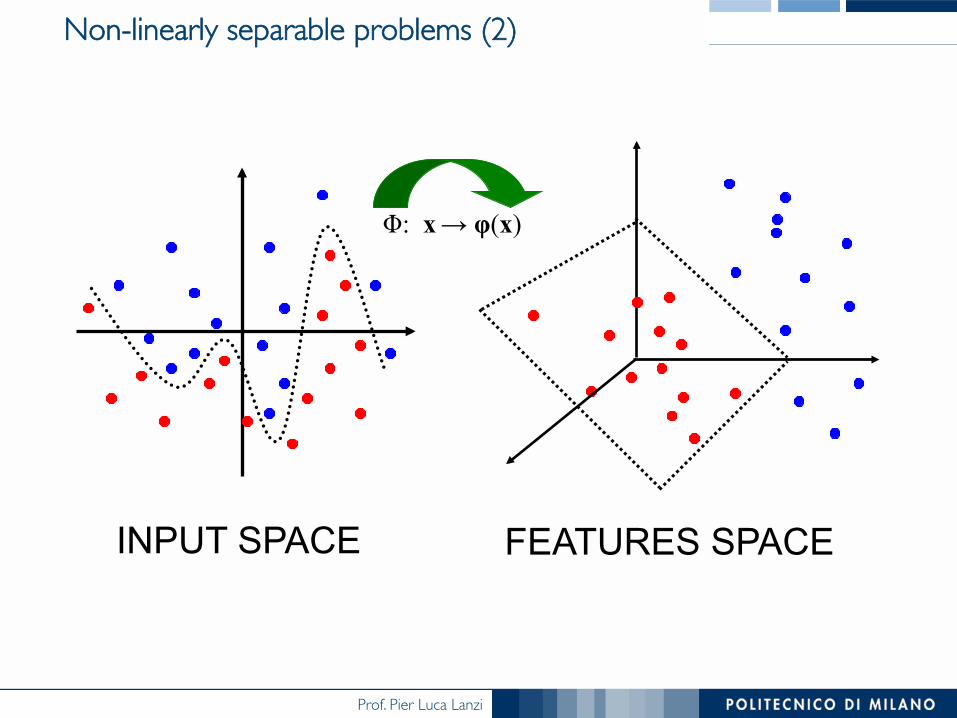
Non-linearly separable problems (2)
Φ: x → φ(x)
INPUT SPACE FEATURES SPACE
Prof. Pier Luca Lanzi
SVMs for Regression
Prof. Pier Luca Lanzi
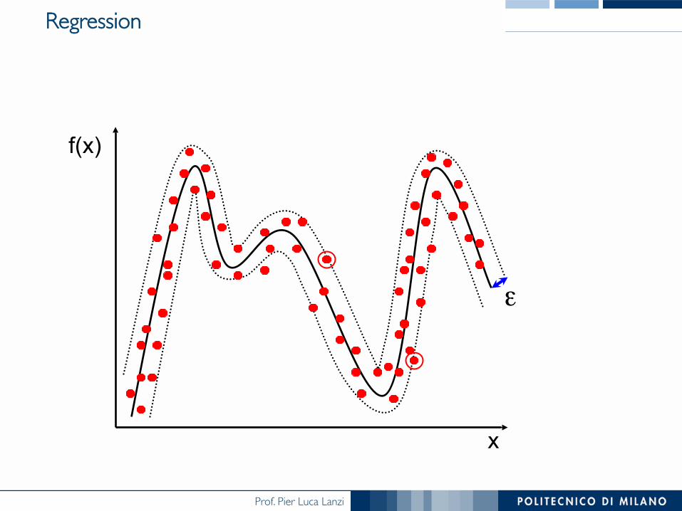
Regression
f(x)
x
ε
Prof. Pier Luca Lanzi
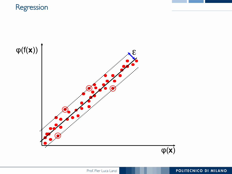
Regression
x
ε
φ(x)
φ(f(x))


![[DBND01] Naive Dreamer - Naive Muse (2010)](https://img.pdfslide.net/doc/110x75/568bda301a28ab2034a9d5d9/dbnd01-naive-dreamer-naive-muse-2010.jpg)