Embed Size (px)
Citation preview

MIS 6324 |Fall-2014|Group 2
1 | P a g e
Predicting delinquency
MIS 6324 Business Intelligence and Software Techniques Fall 2014 -GROUP 2
Submitted by
Arpan Shah
Dipesh Surana
Disha Gujar
Pragati Bora
Narayanan Ramakrishn (RK)
Under the guidance of
Dr.Prof.Radha Mookerjee
The University of Texas at Dallas
In Partial Fulfillment of the Requirements for the Degree of
Masters in Information Technology & Management
MIS 6324 |Fall-2014|Group 2
2 | P a g e
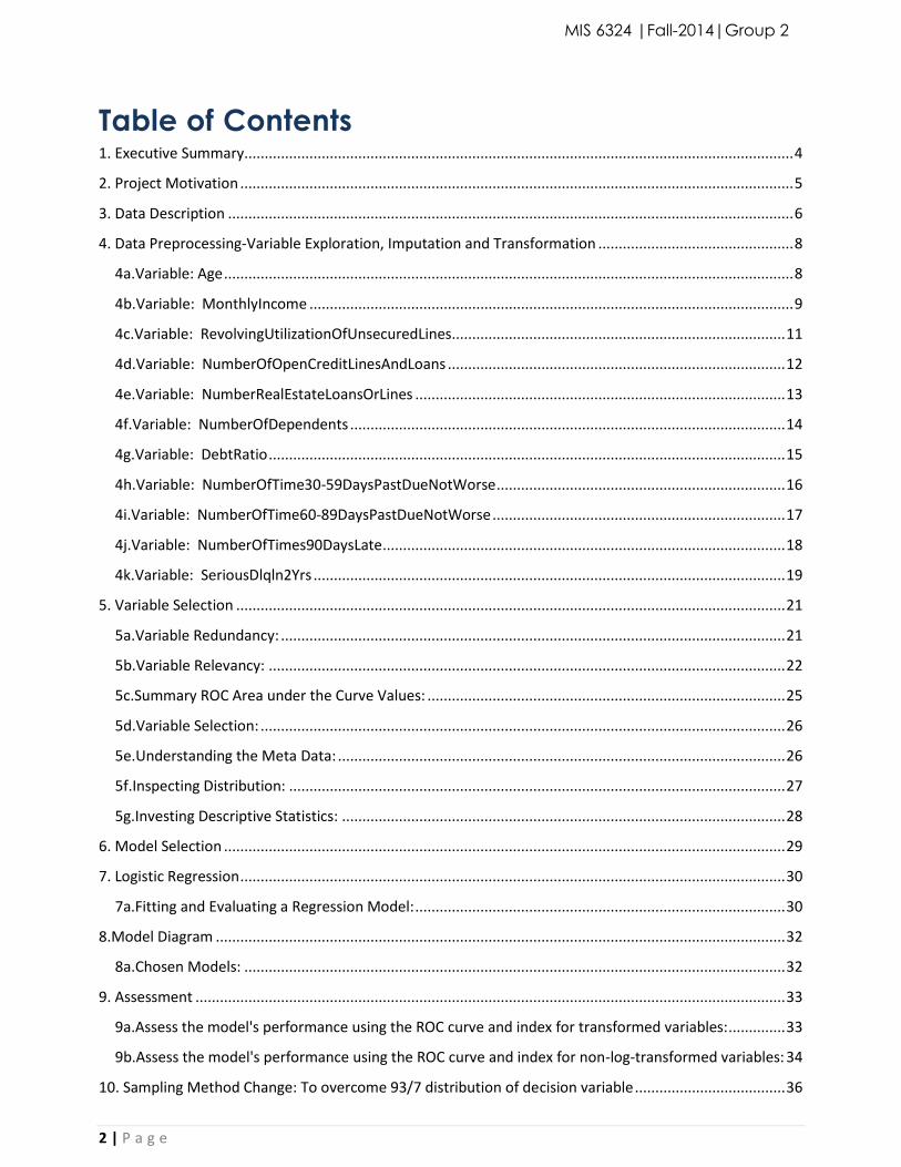
Table of Contents 1. Executive Summary ....................................................................................................................................... 4
2. Project Motivation ........................................................................................................................................ 5
3. Data Description ........................................................................................................................................... 6
4. Data Preprocessing-Variable Exploration, Imputation and Transformation ................................................ 8
4a.Variable: Age ............................................................................................................................................ 8
4b.Variable: MonthlyIncome ....................................................................................................................... 9
4c.Variable: RevolvingUtilizationOfUnsecuredLines .................................................................................. 11
4d.Variable: NumberOfOpenCreditLinesAndLoans ................................................................................... 12
4e.Variable: NumberRealEstateLoansOrLines ........................................................................................... 13
4f.Variable: NumberOfDependents ........................................................................................................... 14
4g.Variable: DebtRatio ............................................................................................................................... 15
4h.Variable: NumberOfTime30-59DaysPastDueNotWorse ....................................................................... 16
4i.Variable: NumberOfTime60-89DaysPastDueNotWorse ........................................................................ 17
4j.Variable: NumberOfTimes90DaysLate ................................................................................................... 18
4k.Variable: SeriousDlqln2Yrs .................................................................................................................... 19
5. Variable Selection ....................................................................................................................................... 21
5a.Variable Redundancy: ............................................................................................................................ 21
5b.Variable Relevancy: ............................................................................................................................... 22
5c.Summary ROC Area under the Curve Values: ........................................................................................ 25
5d.Variable Selection: ................................................................................................................................. 26
5e.Understanding the Meta Data: .............................................................................................................. 26
5f.Inspecting Distribution: .......................................................................................................................... 27
5g.Investing Descriptive Statistics: ............................................................................................................. 28
6. Model Selection .......................................................................................................................................... 29
7. Logistic Regression ...................................................................................................................................... 30
7a.Fitting and Evaluating a Regression Model: ........................................................................................... 30
8.Model Diagram ............................................................................................................................................ 32
8a.Chosen Models: ..................................................................................................................................... 32
9. Assessment ................................................................................................................................................. 33
9a.Assess the model's performance using the ROC curve and index for transformed variables: .............. 33
9b.Assess the model's performance using the ROC curve and index for non-log-transformed variables: 34
10. Sampling Method Change: To overcome 93/7 distribution of decision variable ..................................... 36
MIS 6324 |Fall-2014|Group 2
3 | P a g e
11. Findings ..................................................................................................................................................... 38
12. Conclusion ................................................................................................................................................. 39
13. Managerial Implications: .......................................................................................................................... 40
13a.Putting Accuracy to context - Business Sense ..................................................................................... 40
13b. Business Benefits ................................................................................................................................ 40
14. Attachments ............................................................................................................................................. 41
15. References ................................................................................................................................................ 41
MIS 6324 |Fall-2014|Group 2
4 | P a g e
1. Executive Summary
Banks play a crucial role in market economies. They decide who can get finance and on what
terms and can make or break investment decisions. For markets and society to function,
individuals and companies need access to credit.
Credit scoring algorithms, which make a guess at the probability of default, are the method banks
use to determine whether or not a loan should be granted. This project requires us to improve on
the state of the art in credit scoring, by predicting the probability that somebody will experience
financial distress in the next two years.
In this project, historical data on 150,000 borrowers is analyzed. We implemented various
classification algorithms for predicting whether some-body will experience financial distress in the
next two years by looking on various parameters like monthly income, age, number of open credit
lines and loans etc. An assessment of accuracy of implemented models is also done. Also, data
cleaning approaches used are explained in this report. The model can be used to help in making
best financial decisions when granting loans.

MIS 6324 |Fall-2014|Group 2
5 | P a g e
2. Project Motivation
The problem that we are attempting to solve is a classical one for analytics. It is commonly
desired for banks to accurately assess the probability of default for their customers so that they
can manage their loan risk better. With a better model, they can take calculated Risk in lending
out to customers thus improving the certainty of their profit. They can also tailor make interest rate
to cover for the level of risk they are exposed from the loan. Such models are heavily in demanded
triggered due to the 2008 financial crisis followed by competitive forces and globalization effects
which underscores the importance of business intelligence in financial risk.
However, developing such models still remains a challenge, especially with the growing demand
for consumer loans. Data size is huge, and we are often talking about panel data. Such initiative
necessitates bank to invest in proper data warehouse technologies to support development and
active updating of such models. Also, it is common to see banks using score cards or simple logistic
regression models to evaluate customer risk. This paper will attempt to use traditional analytics
models such as neural network and logistic regression and attempt to create a superior model
using the SEMMA methodology to better predict customers default.
The data is based on real consumer loan data. The data mining models also include decision tree,
neural networks and traditional logistic regression. In addition, we will conduct uni-variate and
multivariate analysis of data to identify insights into banking customers.
The details of the various techniques and data cleaning approach used are given in subsequent
sections in this paper.
MIS 6324 |Fall-2014|Group 2
6 | P a g e
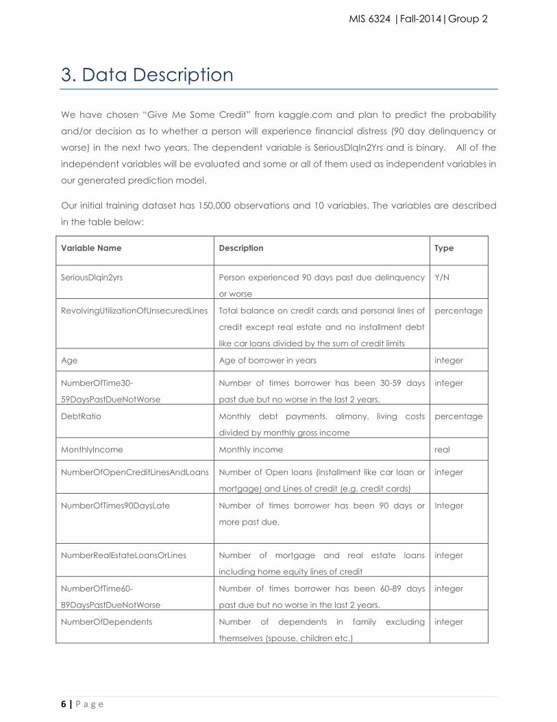
3. Data Description
We have chosen “Give Me Some Credit” from kaggle.com and plan to predict the probability
and/or decision as to whether a person will experience financial distress (90 day delinquency or
worse) in the next two years. The dependent variable is SeriousDlqIn2Yrs and is binary. All of the
independent variables will be evaluated and some or all of them used as independent variables in
our generated prediction model.
Our initial training dataset has 150,000 observations and 10 variables. The variables are described
in the table below:
Variable Name Description Type
SeriousDlqin2yrs Person experienced 90 days past due delinquency
or worse
Y/N
RevolvingUtilizationOfUnsecuredLines Total balance on credit cards and personal lines of
credit except real estate and no installment debt
like car loans divided by the sum of credit limits
percentage
Age Age of borrower in years integer
NumberOfTime30-
59DaysPastDueNotWorse
Number of times borrower has been 30-59 days
past due but no worse in the last 2 years.
integer
DebtRatio Monthly debt payments, alimony, living costs
divided by monthly gross income
percentage
MonthlyIncome Monthly income real
NumberOfOpenCreditLinesAndLoans Number of Open loans (installment like car loan or
mortgage) and Lines of credit (e.g. credit cards)
integer
NumberOfTimes90DaysLate Number of times borrower has been 90 days or
more past due.
Integer
NumberRealEstateLoansOrLines Number of mortgage and real estate loans
including home equity lines of credit
integer
NumberOfTime60-
89DaysPastDueNotWorse
Number of times borrower has been 60-89 days
past due but no worse in the last 2 years.
integer
NumberOfDependents Number of dependents in family excluding
themselves (spouse, children etc.)
integer
MIS 6324 |Fall-2014|Group 2
7 | P a g e
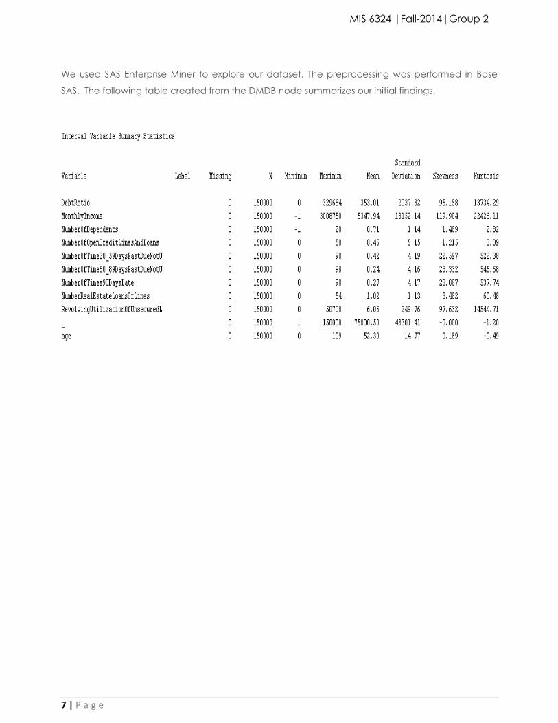
We used SAS Enterprise Miner to explore our dataset. The preprocessing was performed in Base
SAS. The following table created from the DMDB node summarizes our initial findings.
MIS 6324 |Fall-2014|Group 2
8 | P a g e
4. Data Preprocessing-Variable Exploration,
Imputation and Transformation
We also went on to graph each variable to get a better understanding of its distribution and
outliers. The following is a summary of each variable with its initial histogram and observations, an
explanation of the data clean up that was completed to remove outliers and/or missing values,
and our observations and a histogram of the variable after transforming it.
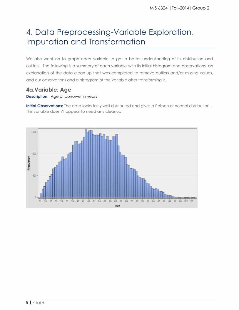
4a.Variable: Age Description: Age of borrower in years
Initial Observations: The data looks fairly well distributed and gives a Poisson or normal distribution.
This variable doesn’t appear to need any cleanup.
MIS 6324 |Fall-2014|Group 2
9 | P a g e
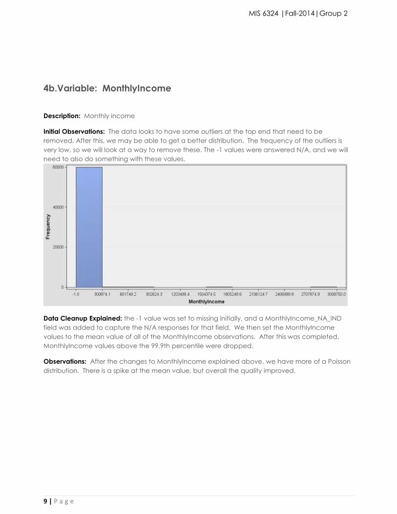
4b.Variable: MonthlyIncome
Description: Monthly income
Initial Observations: The data looks to have some outliers at the top end that need to be
removed. After this, we may be able to get a better distribution. The frequency of the outliers is
very low, so we will look at a way to remove these. The -1 values were answered N/A, and we will
need to also do something with these values.
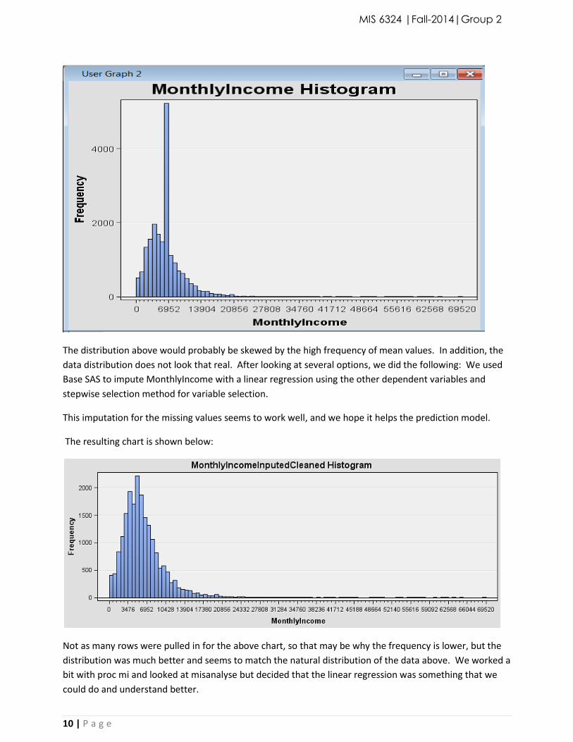
Data Cleanup Explained: the -1 value was set to missing initially, and a MonthlyIncome_NA_IND
field was added to capture the N/A responses for that field. We then set the MonthlyIncome
values to the mean value of all of the MonthlyIncome observations. After this was completed,
MonthlyIncome values above the 99.9th percentile were dropped.
Observations: After the changes to MonthlyIncome explained above, we have more of a Poisson
distribution. There is a spike at the mean value, but overall the quality improved.
MIS 6324 |Fall-2014|Group 2
10 | P a g e
The distribution above would probably be skewed by the high frequency of mean values. In addition, the
data distribution does not look that real. After looking at several options, we did the following: We used
Base SAS to impute MonthlyIncome with a linear regression using the other dependent variables and
stepwise selection method for variable selection.
This imputation for the missing values seems to work well, and we hope it helps the prediction model.
The resulting chart is shown below:
Not as many rows were pulled in for the above chart, so that may be why the frequency is lower, but the
distribution was much better and seems to match the natural distribution of the data above. We worked a
bit with proc mi and looked at misanalyse but decided that the linear regression was something that we
could do and understand better.
MIS 6324 |Fall-2014|Group 2
11 | P a g e
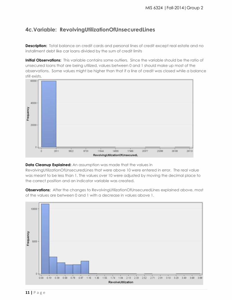
4c.Variable: RevolvingUtilizationOfUnsecuredLines
Description: Total balance on credit cards and personal lines of credit except real estate and no
installment debt like car loans divided by the sum of credit limits
Initial Observations: This variable contains some outliers. Since the variable should be the ratio of
unsecured loans that are being utilized, values between 0 and 1 should make up most of the
observations. Some values might be higher than that if a line of credit was closed while a balance
still exists.
Data Cleanup Explained: An assumption was made that the values in
RevolvingUtilizationOfUnsecuredLines that were above 10 were entered in error. The real value
was meant to be less than 1. The values over 10 were adjusted by moving the decimal place to
the correct position and an indicator variable was created.
Observations: After the changes to RevolvingUtilizationOfUnsecuredLines explained above, most
of the values are between 0 and 1 with a decrease in values above 1.
MIS 6324 |Fall-2014|Group 2
12 | P a g e
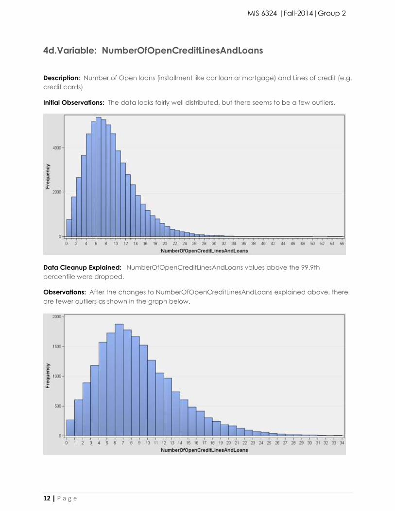
4d.Variable: NumberOfOpenCreditLinesAndLoans
Description: Number of Open loans (installment like car loan or mortgage) and Lines of credit (e.g.
credit cards)
Initial Observations: The data looks fairly well distributed, but there seems to be a few outliers.
Data Cleanup Explained: NumberOfOpenCreditLinesAndLoans values above the 99.9th
percentile were dropped.
Observations: After the changes to NumberOfOpenCreditLinesAndLoans explained above, there
are fewer outliers as shown in the graph below.
MIS 6324 |Fall-2014|Group 2
13 | P a g e
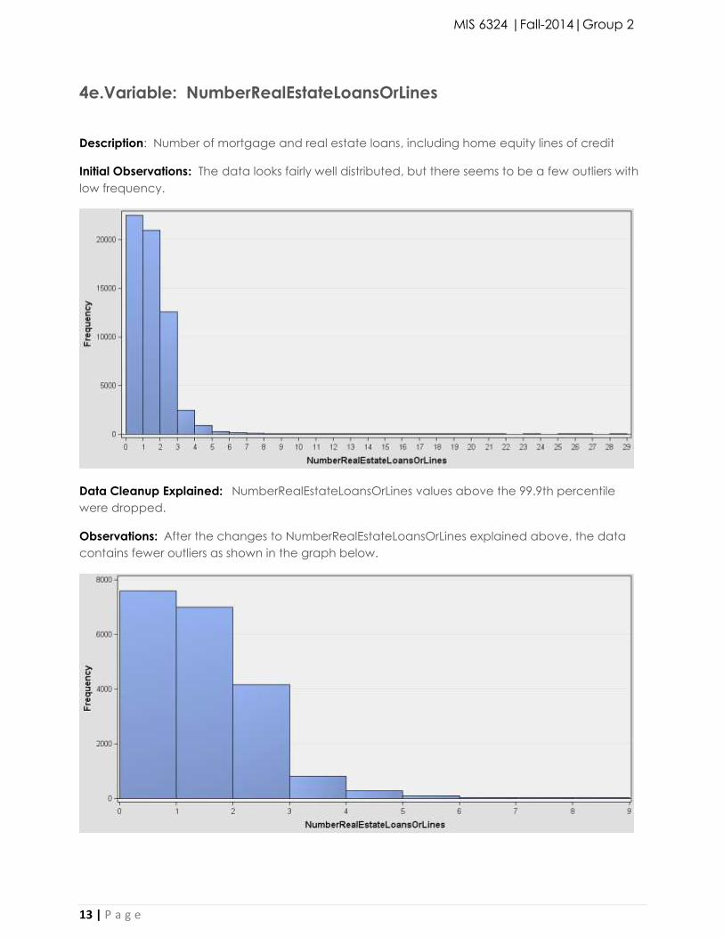
4e.Variable: NumberRealEstateLoansOrLines
Description: Number of mortgage and real estate loans, including home equity lines of credit
Initial Observations: The data looks fairly well distributed, but there seems to be a few outliers with
low frequency.
Data Cleanup Explained: NumberRealEstateLoansOrLines values above the 99.9th percentile
were dropped.
Observations: After the changes to NumberRealEstateLoansOrLines explained above, the data
contains fewer outliers as shown in the graph below.
MIS 6324 |Fall-2014|Group 2
14 | P a g e
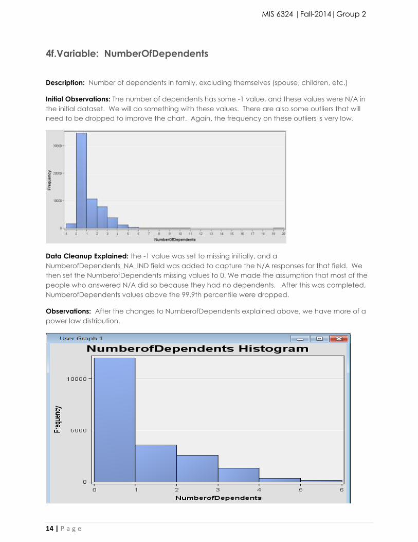
4f.Variable: NumberOfDependents
Description: Number of dependents in family, excluding themselves (spouse, children, etc.)
Initial Observations: The number of dependents has some -1 value, and these values were N/A in
the initial dataset. We will do something with these values. There are also some outliers that will
need to be dropped to improve the chart. Again, the frequency on these outliers is very low.
Data Cleanup Explained: the -1 value was set to missing initially, and a
NumberofDependents_NA_IND field was added to capture the N/A responses for that field. We
then set the NumberofDependents missing values to 0. We made the assumption that most of the
people who answered N/A did so because they had no dependents. After this was completed,
NumberofDependents values above the 99.9th percentile were dropped.
Observations: After the changes to NumberofDependents explained above, we have more of a
power law distribution.
MIS 6324 |Fall-2014|Group 2
15 | P a g e
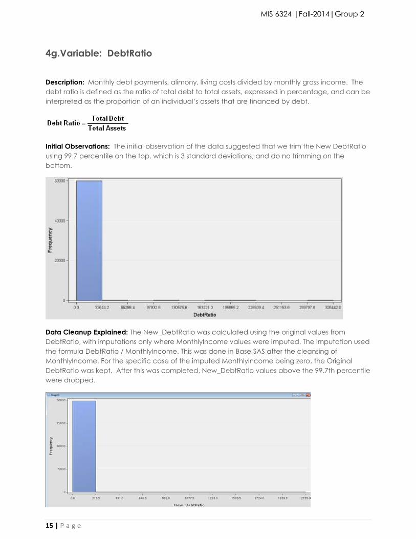
4g.Variable: DebtRatio
Description: Monthly debt payments, alimony, living costs divided by monthly gross income. The
debt ratio is defined as the ratio of total debt to total assets, expressed in percentage, and can be
interpreted as the proportion of an individual’s assets that are financed by debt.
Initial Observations: The initial observation of the data suggested that we trim the New DebtRatio
using 99.7 percentile on the top, which is 3 standard deviations, and do no trimming on the
bottom.
Data Cleanup Explained: The New_DebtRatio was calculated using the original values from
DebtRatio, with imputations only where MonthlyIncome values were imputed. The imputation used
the formula DebtRatio / MonthlyIncome. This was done in Base SAS after the cleansing of
MonthlyIncome. For the specific case of the imputed MonthlyIncome being zero, the Original
DebtRatio was kept. After this was completed, New_DebtRatio values above the 99.7th percentile
were dropped.
MIS 6324 |Fall-2014|Group 2
16 | P a g e
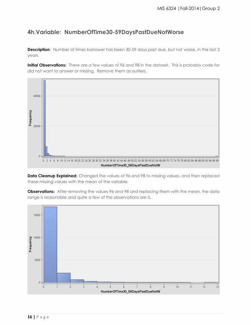
4h.Variable: NumberOfTime30-59DaysPastDueNotWorse
Description: Number of times borrower has been 30-59 days past due, but not worse, in the last 2
years.
Initial Observations: There are a few values of 96 and 98 in the dataset. This is probably code for
did not want to answer or missing. Remove them as outliers.
Data Cleanup Explained: Changed the values of 96 and 98 to missing values, and then replaced
these missing values with the mean of the variable.
Observations: After removing the values 96 and 98 and replacing them with the mean, the data
range is reasonable and quite a few of the observations are 0.
MIS 6324 |Fall-2014|Group 2
17 | P a g e
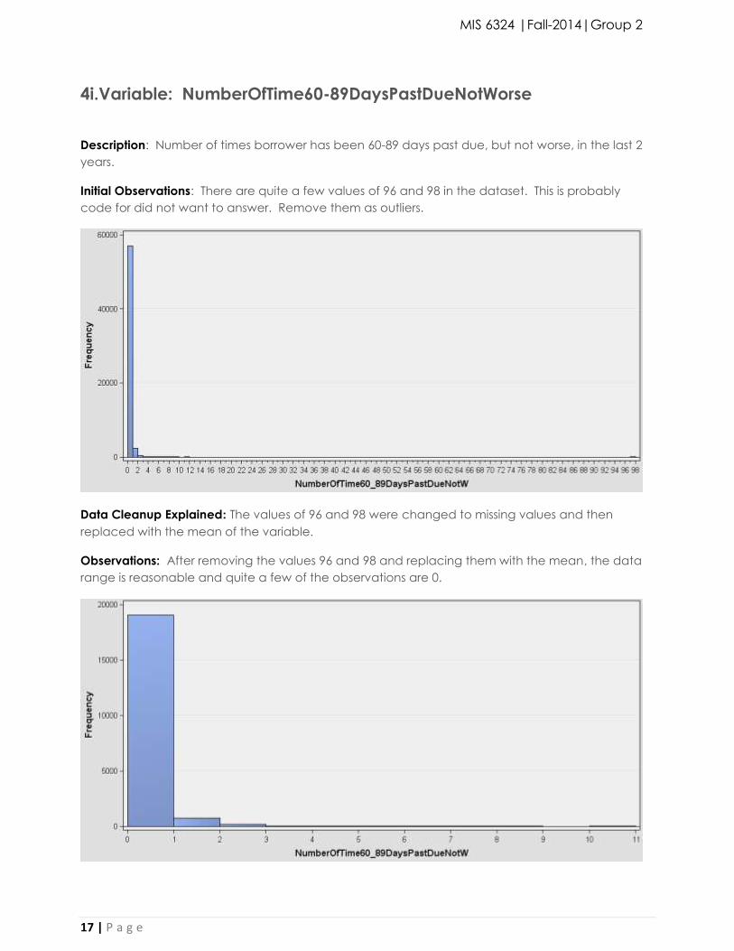
4i.Variable: NumberOfTime60-89DaysPastDueNotWorse
Description: Number of times borrower has been 60-89 days past due, but not worse, in the last 2
years.
Initial Observations: There are quite a few values of 96 and 98 in the dataset. This is probably
code for did not want to answer. Remove them as outliers.
Data Cleanup Explained: The values of 96 and 98 were changed to missing values and then
replaced with the mean of the variable.
Observations: After removing the values 96 and 98 and replacing them with the mean, the data
range is reasonable and quite a few of the observations are 0.
MIS 6324 |Fall-2014|Group 2
18 | P a g e
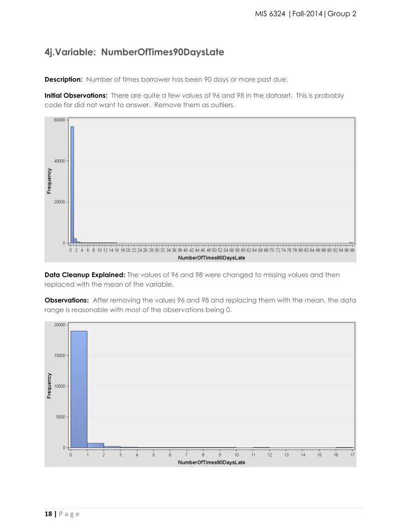
4j.Variable: NumberOfTimes90DaysLate
Description: Number of times borrower has been 90 days or more past due.
Initial Observations: There are quite a few values of 96 and 98 in the dataset. This is probably
code for did not want to answer. Remove them as outliers.
Data Cleanup Explained: The values of 96 and 98 were changed to missing values and then
replaced with the mean of the variable.
Observations: After removing the values 96 and 98 and replacing them with the mean, the data
range is reasonable with most of the observations being 0.
MIS 6324 |Fall-2014|Group 2
19 | P a g e
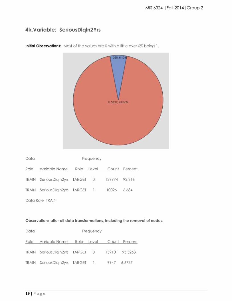
4k.Variable: SeriousDlqln2Yrs
Initial Observations: Most of the values are 0 with a little over 6% being 1.
Data Frequency
Role Variable Name Role Level Count Percent
TRAIN SeriousDlqin2yrs TARGET 0 139974 93.316
TRAIN SeriousDlqin2yrs TARGET 1 10026 6.684
Data Role=TRAIN
Observations after all data transformations, including the removal of nodes:
Data Frequency
Role Variable Name Role Level Count Percent
TRAIN SeriousDlqin2yrs TARGET 0 139101 93.3263
TRAIN SeriousDlqin2yrs TARGET 1 9947 6.6737
MIS 6324 |Fall-2014|Group 2
20 | P a g e
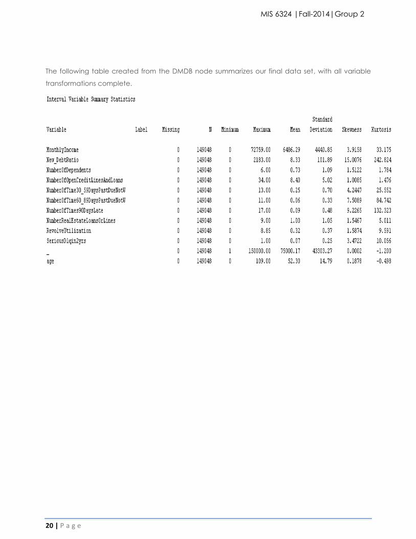
The following table created from the DMDB node summarizes our final data set, with all variable
transformations complete.
MIS 6324 |Fall-2014|Group 2
21 | P a g e
5. Variable Selection
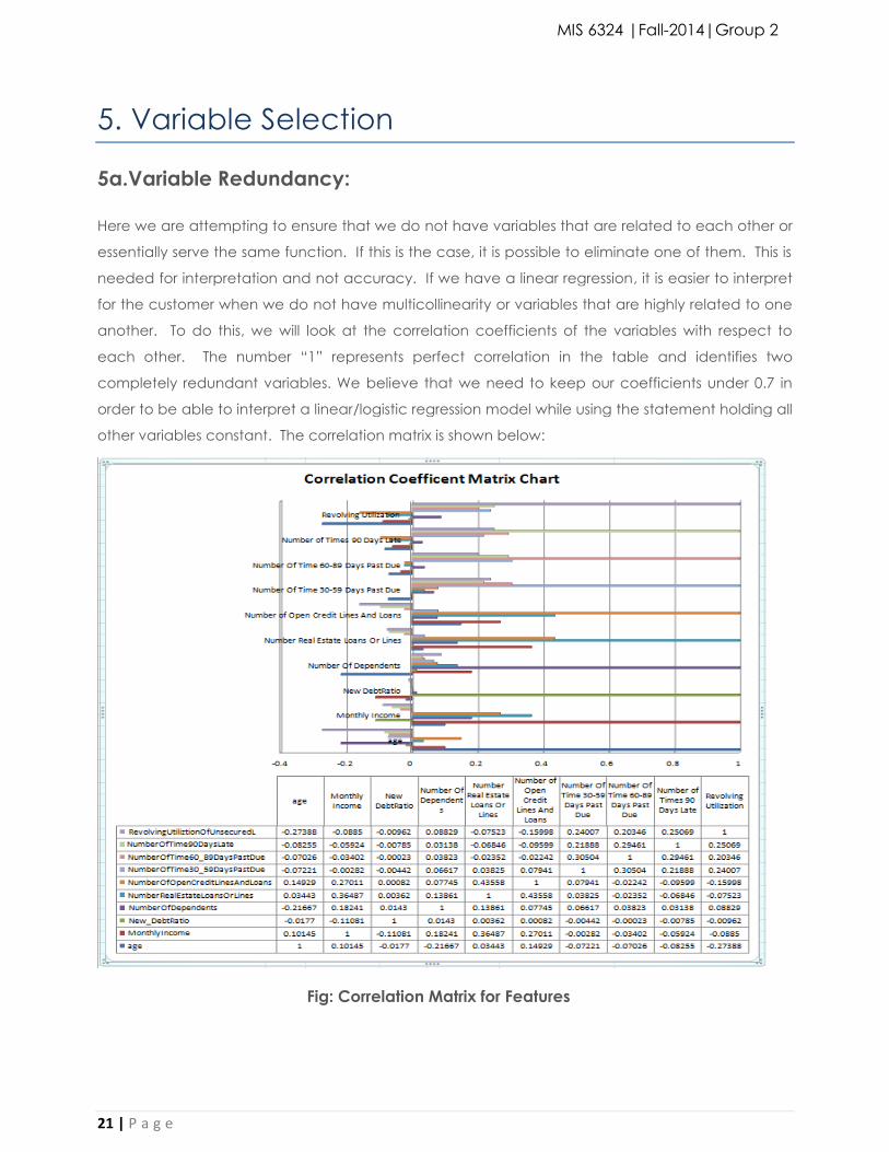
5a.Variable Redundancy:
Here we are attempting to ensure that we do not have variables that are related to each other or
essentially serve the same function. If this is the case, it is possible to eliminate one of them. This is
needed for interpretation and not accuracy. If we have a linear regression, it is easier to interpret
for the customer when we do not have multicollinearity or variables that are highly related to one
another. To do this, we will look at the correlation coefficients of the variables with respect to
each other. The number “1” represents perfect correlation in the table and identifies two
completely redundant variables. We believe that we need to keep our coefficients under 0.7 in
order to be able to interpret a linear/logistic regression model while using the statement holding all
other variables constant. The correlation matrix is shown below:
Fig: Correlation Matrix for Features
MIS 6324 |Fall-2014|Group 2
22 | P a g e
In the correlation matrix, we ignore the 1’s as those are a variable that is correlated against it. The
highest is NumberofOpenCreditLinesAndLoans and NumberRealEstateLoansOrLines at 0 .44. This is
not too high, and for interpretability we should be able to interpret a linear equation if we do not
take the log or execute another complex function on the features. It does not appear that there
are any variables that need to be removed for multicollinearity.
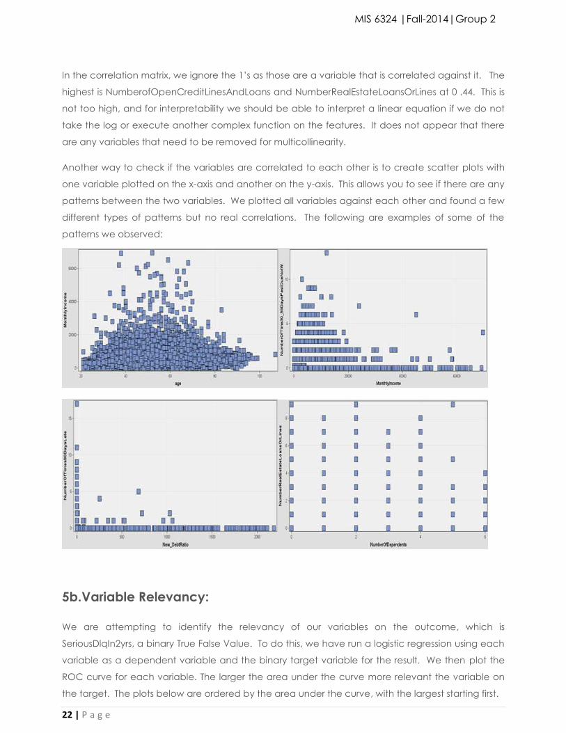
Another way to check if the variables are correlated to each other is to create scatter plots with
one variable plotted on the x-axis and another on the y-axis. This allows you to see if there are any
patterns between the two variables. We plotted all variables against each other and found a few
different types of patterns but no real correlations. The following are examples of some of the
patterns we observed:
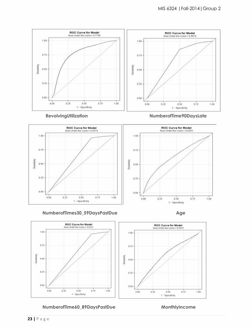
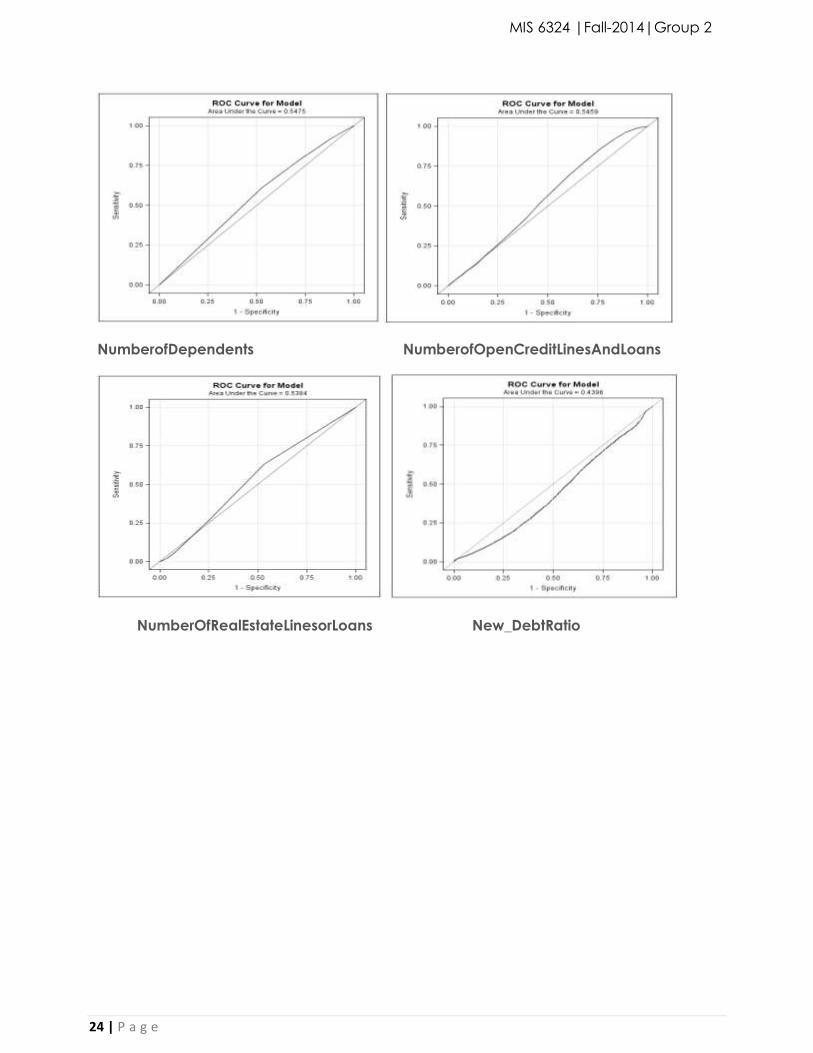
5b.Variable Relevancy:
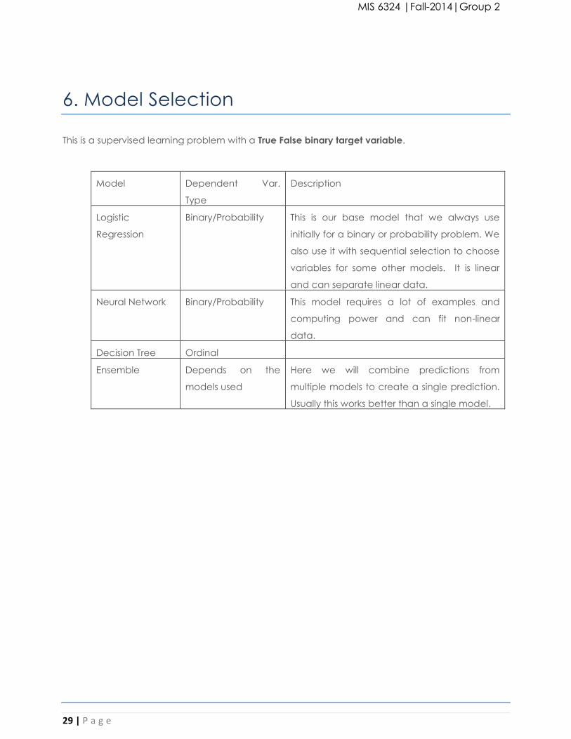
We are attempting to identify the relevancy of our variables on the outcome, which is
SeriousDlqIn2yrs, a binary True False Value. To do this, we have run a logistic regression using each
variable as a dependent variable and the binary target variable for the result. We then plot the
ROC curve for each variable. The larger the area under the curve more relevant the variable on
the target. The plots below are ordered by the area under the curve, with the largest starting first.
MIS 6324 |Fall-2014|Group 2
23 | P a g e
RevolvingUtilization NumberofTime90DaysLate
NumberofTimes30_59DaysPastDue Age
NumberofTime60_89DaysPastDue MonthlyIncome
MIS 6324 |Fall-2014|Group 2
24 | P a g e
NumberofDependents NumberofOpenCreditLinesAndLoans
NumberOfRealEstateLinesorLoans New_DebtRatio
MIS 6324 |Fall-2014|Group 2
25 | P a g e
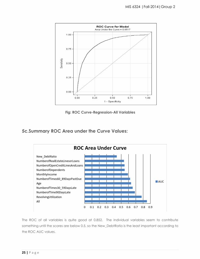
Fig: ROC Curve-Regression-All Variables
5c.Summary ROC Area under the Curve Values:
The ROC of all variables is quite good at 0.852. The individual variables seem to contribute
something until the scores are below 0.5, so the New_DebtRatio is the least important according to
the ROC AUC values.
MIS 6324 |Fall-2014|Group 2
26 | P a g e
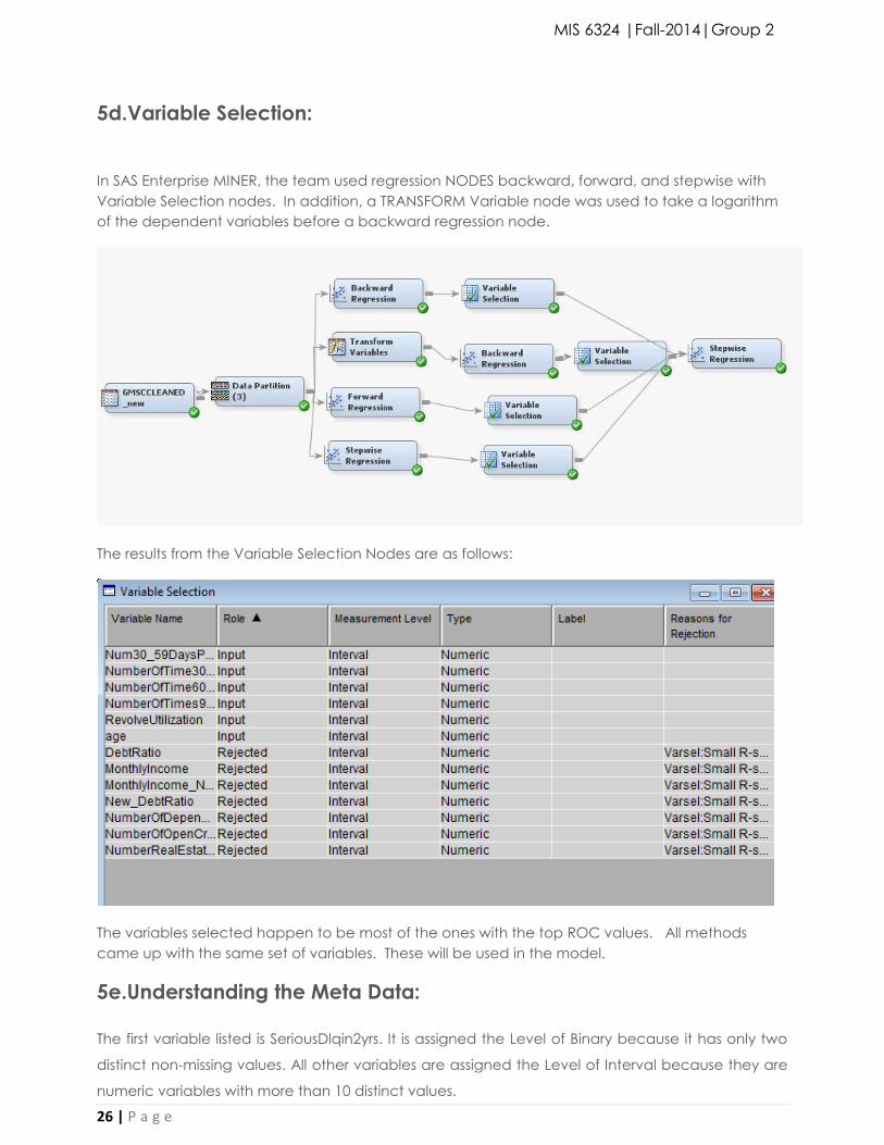
5d.Variable Selection:
In SAS Enterprise MINER, the team used regression NODES backward, forward, and stepwise with
Variable Selection nodes. In addition, a TRANSFORM Variable node was used to take a logarithm
of the dependent variables before a backward regression node.
The results from the Variable Selection Nodes are as follows:
The variables selected happen to be most of the ones with the top ROC values. All methods
came up with the same set of variables. These will be used in the model.
5e.Understanding the Meta Data:
The first variable listed is SeriousDlqin2yrs. It is assigned the Level of Binary because it has only two
distinct non-missing values. All other variables are assigned the Level of Interval because they are
numeric variables with more than 10 distinct values.
MIS 6324 |Fall-2014|Group 2
27 | P a g e
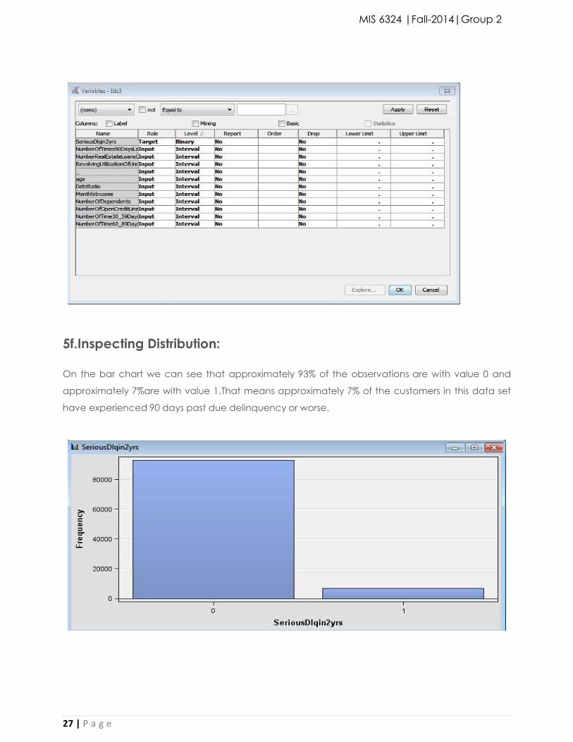
5f.Inspecting Distribution:
On the bar chart we can see that approximately 93% of the observations are with value 0 and
approximately 7%are with value 1.That means approximately 7% of the customers in this data set
have experienced 90 days past due delinquency or worse.
28 | P a g e
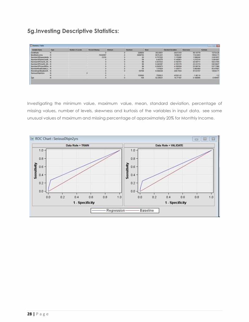
5g.Investing Descriptive Statistics:
Investigating the minimum value, maximum value, mean, standard deviation, percentage of
missing values, number of levels, skewness and kurtosis of the variables in input data, see some
unusual values of maximum and missing percentage of approximately 20% for Monthly Income.
MIS 6324 |Fall-2014|Group 2
29 | P a g e
6. Model Selection
This is a supervised learning problem with a True False binary target variable.
Model Dependent Var.
Type
Description
Logistic
Regression
Binary/Probability This is our base model that we always use
initially for a binary or probability problem. We
also use it with sequential selection to choose
variables for some other models. It is linear
and can separate linear data.
Neural Network Binary/Probability This model requires a lot of examples and
computing power and can fit non-linear
data.
Decision Tree Ordinal
Ensemble Depends on the
models used
Here we will combine predictions from
multiple models to create a single prediction.
Usually this works better than a single model.
MIS 6324 |Fall-2014|Group 2
30 | P a g e
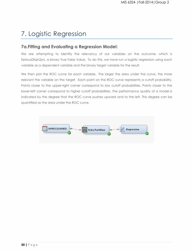
7. Logistic Regression
7a.Fitting and Evaluating a Regression Model:
We are attempting to identify the relevancy of our variables on the outcome, which is
SeriousDlqIn2yrs, a binary True False Value. To do this, we have run a logistic regression using each
variable as a dependent variable and the binary target variable for the result.
We then plot the ROC curve for each variable. The larger the area under the curve, the more
relevant the variable on the target. Each point on the ROC curve represents a cutoff probability.
Points closer to the upper-right corner correspond to low cutoff probabilities. Points closer to the
lower-left corner correspond to higher cutoff probabilities. The performance quality of a model is
indicated by the degree that the ROC curve pushes upward and to the left. This degree can be
quantified as the area under the ROC curve.
MIS 6324 |Fall-2014|Group 2
31 | P a g e
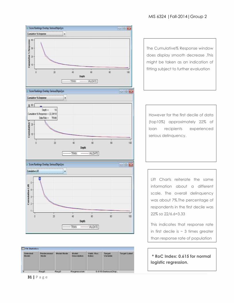
The Cumulative% Response window
does display smooth decrease .This
might be taken as an indication of
fitting subject to further evaluation
However for the first decile of data
(top10%) approximately 22% of
loan recipients experienced
serious delinquency.
(
T
h
i
s
c
a
n
b
e
l
i
n
k
e
d
w
i
t
h
i
n
Lift Charts reiterate the same
information about a different
scale. The overall delinquency
was about 7%.The percentage of
respondents in the first decile was
22% so 22/6.6=3.33
This indicates that response rate
in first decile is ~ 3 times greater
than response rate of population
* RoC Index: 0.615 for normal
logistic regression.
MIS 6324 |Fall-2014|Group 2
32 | P a g e
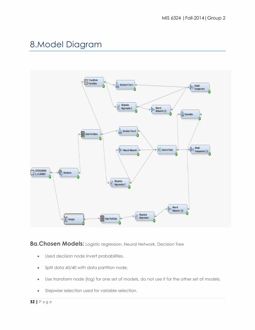
8.Model Diagram
8a.Chosen Models: Logistic regression, Neural Network, Decision Tree
Used decision node invert probabilities.
Split data 60/40 with data partition node.
Use transform node (log) for one set of models, do not use it for the other set of models.
Stepwise selection used for variable selection.
MIS 6324 |Fall-2014|Group 2
33 | P a g e
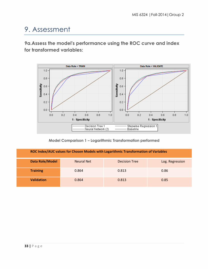
9. Assessment
9a.Assess the model's performance using the ROC curve and index
for transformed variables:
Model Comparison 1 – Logarithmic Transformation performed
ROC Index/AUC values for Chosen Models with Logarithmic Transformation of Variables
Data Role/Model Neural Net Decision Tree Log. Regression
Training 0.864 0.813 0.86
Validation 0.864 0.813 0.85
MIS 6324 |Fall-2014|Group 2
34 | P a g e
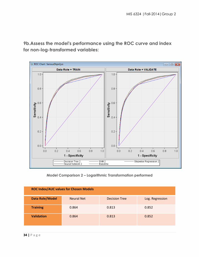
9b.Assess the model's performance using the ROC curve and index
for non-log-transformed variables:
Model Comparison 2 – Logarithmic Transformation performed
ROC Index/AUC values for Chosen Models
Data Role/Model Neural Net Decision Tree Log. Regression
Training 0.864 0.813 0.852
Validation 0.864 0.813 0.852
MIS 6324 |Fall-2014|Group 2
35 | P a g e
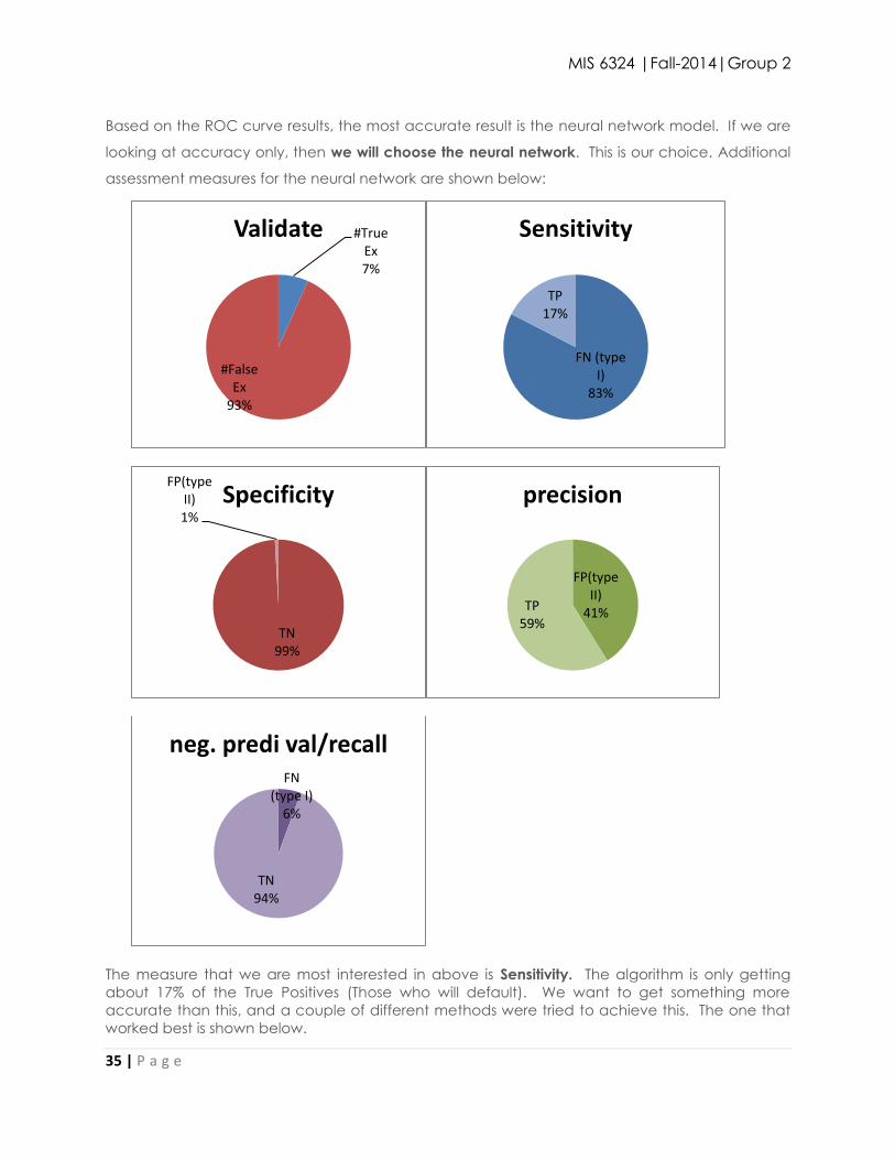
Based on the ROC curve results, the most accurate result is the neural network model. If we are
looking at accuracy only, then we will choose the neural network. This is our choice. Additional
assessment measures for the neural network are shown below:
The measure that we are most interested in above is Sensitivity. The algorithm is only getting
about 17% of the True Positives (Those who will default). We want to get something more
accurate than this, and a couple of different methods were tried to achieve this. The one that
worked best is shown below.
#True Ex 7%
#False Ex
93%
Validate
FN (type I)
83%
TP 17%
Sensitivity
TN 99%
FP(type II) 1%
Specificity
FP(type II)
41% TP 59%
precision
FN (type I)
6%
TN 94%
neg. predi val/recall
MIS 6324 |Fall-2014|Group 2
36 | P a g e
10. Sampling Method Change: To overcome
93/7 distribution of decision variable
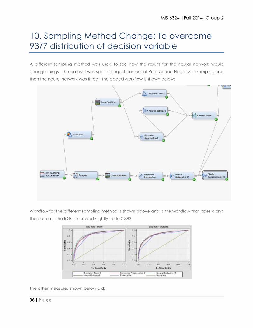
A different sampling method was used to see how the results for the neural network would
change things. The dataset was split into equal portions of Positive and Negative examples, and
then the neural network was fitted. The added workflow is shown below:
Workflow for the different sampling method is shown above and is the workflow that goes along
the bottom. The ROC improved slightly up to 0.883.
The other measures shown below did:
MIS 6324 |Fall-2014|Group 2
37 | P a g e
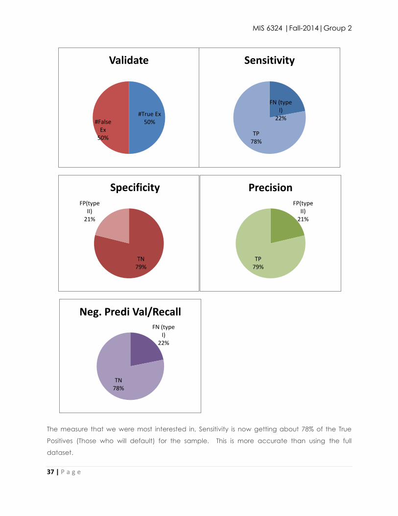
The measure that we were most interested in, Sensitivity is now getting about 78% of the True
Positives (Those who will default) for the sample. This is more accurate than using the full
dataset.
#True Ex 50% #False
Ex 50%
Validate
FN (type I)
22%
TP 78%
Sensitivity
TN 79%
FP(type II)
21%
Specificity FP(type
II) 21%
TP 79%
Precision
FN (type I)
22%
TN 78%
Neg. Predi Val/Recall
MIS 6324 |Fall-2014|Group 2
38 | P a g e
11. Findings
In accordance with to the SEMMA methodology, after obtaining the sample data we started by
exploring the data .We found that Histograms were very useful in Exploring and
understanding the spread of the data. Also, skewness of the data has significant effect on
analysis. So, different methods need to be implemented to overcome such shortcomings of the
dataset. Also, dealing with missing values is an important step of data cleaning. Different
methods like mean, percentile, regression were used to treat the missing values. Also
other techniques like scatter plots, correlation were used to identify variable relevancy
and importance. When modifying the data we followed tried logarithmic
transformations, although they did not impact our findings. We further modeled our data
using various classification techniques like logarithmic regression, decision trees,
Neural Networks. Then when assessing the various techniques, we used ROC Index,
Precision, Recall, Sensitivity, etc. to compare the results. ROC values were almost
similar for most of the techniques but the results were not great in terms of Sensitivity. This was
because of the 93:7 proportion of events .So, on changing the sampling method; we were able
to get better results of about 78% of the True Positives (Those who will default) for the
sample this is more accurate.

MIS 6324 |Fall-2014|Group 2
39 | P a g e
12. Conclusion
In conclusion, we have shown that it is possible to use superior analytics algorithm through the
use of ensemble methods to correctly classify customers according to their probability of
default. We believe our neural network ensemble model is as close to the true model as possible.
Such model can be easily updated within a single data and would have the capability to scale
up for banking usage in the commercial world. We are confident that development and up-
keeping of this model will help the bank gain extra profitability.
MIS 6324 |Fall-2014|Group 2
40 | P a g e
13. Managerial Implications:
13a.Putting Accuracy to context - Business Sense • Examining a slice of the customer database (150,000 customers) we find that 6.6% of
customers were seriously delinquent in payment the last two years
• If only 5% of their carried debt was the store credit card this is potentially an:
― Average loss of $8.12 per customer
― Potential overall loss of $1.2 million
• This could be used to decrease credit limits or cancel credit lines for current risky
customers to minimize potential loss
• We could save $600,000 over two years if we correctly predicted 50% of the customers
that would default and changed their account to prevent it
• The potential loss is minimized by ~$8,000 for every 100,000 customers with each
percentage point increase in accuracy
13b. Business Benefits
• Product Mangers can closely monitor the customer behavior and determine limits per
account accordingly
• Monitoring Corporate or cardholders behavior to identify payment realization problems
in initial stage itself and thereby eliminate the credit risk
• Transaction monitoring facilitates strategy making for corrective actions or raises an
alarm to avoid further increase in Delinquency
• Model forecast monthly delinquency through predictive scores and helps in right
targeting and effort optimization for reducing delinquency.
MIS 6324 |Fall-2014|Group 2
41 | P a g e
14. Attachments
BASE SAS Code:
Final Code.txt
15. References
https://www.kaggle.com/c/GiveMeSomeCredit
http://support.sas.com/rnd/base/index.html
http://www.iaesjournal.com/online/index.php/TELKOMNIKA/article/viewFile/1323/pdf
http://www.solvith.com/Credit%20Default.pdf
https://www.youtube.com/watch?v=cggp8EoGN4Y
http://cs.jhu.edu/~vmohan3/document/ml_financial.pdf
http://www.sas.com/en_us/software/analytics/enterprise-miner.html
Data Mining for Business Intelligence: Concepts, Techniques, and Applications in
Microsoft Office Excel® with XLMiner®, 2nd Edition by-Galit Shmueli, Nitin R. Patel, Peter
C. Bruce