1

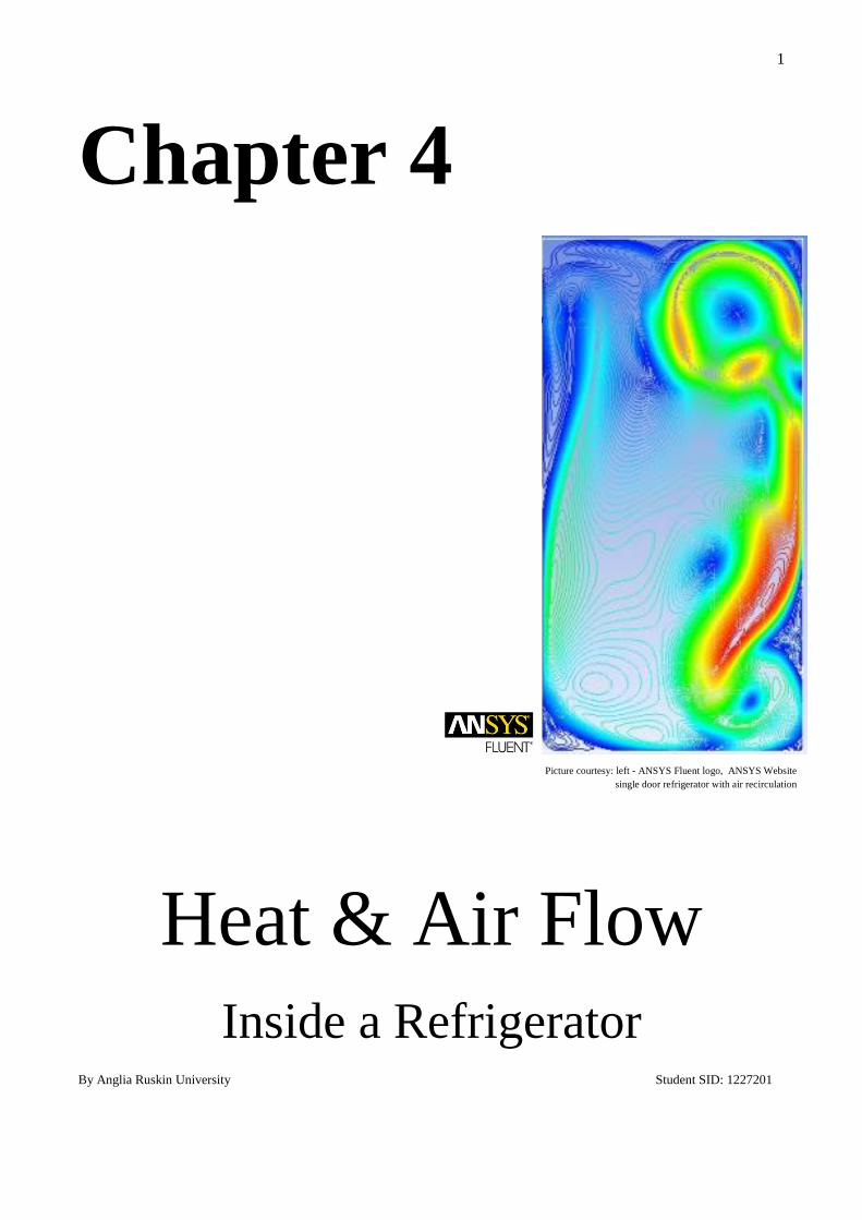
Chapter 4

Heat & Air Flow

Inside a Refrigerator By Anglia Ruskin University Student SID: 1227201

Picture courtesy: left - ANSYS Fluent logo, ANSYS Website

single door refrigerator with air recirculation

2

Table of Contents

Table of figures................................................................................................................................................ 3

Introduction ..................................................................................................................................................... 4

Basics types of domestic refrigerators ............................................................................................................. 4

Literature Review: ........................................................................................................................................... 5

Airflow near a Vertical Plate: ...................................................................................................................... 6

Air Flow in empty closed cavity and heat transfer: ..................................................................................... 7

Air Flow recirculation in a refrigerator ....................................................................................................... 7

Basic of airflow: ...................................................................................................................................... 7

Relation of heat and airflow in a refrigerator .............................................................................................. 9

Effect of door ajar on airflow and temperature of a refrigerator ............................................................... 10

Effect of compressor on & off mode on temperature. ............................................................................... 10

Energy loss in refrigerator cavity .............................................................................................................. 11

Methodology - Using Fluent CFD for case study .......................................................................................... 13

Pre Processing ........................................................................................................................................... 13

Boundary Conditions ............................................................................................................................. 13

Meshing ................................................................................................................................................. 15

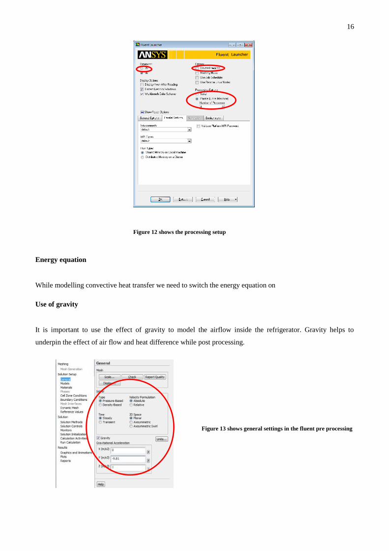
General Settings ......................................................................................................................................... 15

Energy equation ..................................................................................................................................... 16

Use of gravity ........................................................................................................................................ 16

Convergence .......................................................................................................................................... 17

Post Processing - Airflow analysis inside a refrigerator ............................................................................ 17

Case 1: Side wall cold and door warm with top and bottom walls as zero heat flux (no fan) ............... 18

Case 2: Top wall cold and bottom wall warm with both sides to be zero heat flux with a fan ............. 19

Case 3: Top wall warm and bottom wall cold along with sidewalls as zero heat flux along with fan .. 20

Results & Conclusion: ................................................................................................................................... 21

References ..................................................................................................................................................... 22

3

Table of figures

Figure 1 a) Static refrigerator b) Brewed Refrigerator c) No Frost refrigerator ........................................ 5

Figure 2 shows the vertical plate with an air flow in y axis ................................................................................ 6

Figure 3 shows the boundary layer and the velocity profile in natural convection ............................................. 7

Figure 4 shows the laminar and turbulent flow of air .......................................................................................... 8

Figure 5 shows the heat exchange and air flow in the refrigerator cavity ........................................................... 9

Figure 6 shows temperature fluctuation with in with compressor on - off ........................................................ 11

Figure 7 shows a) changes in energy efficiency b) thermal efficiency c) cycle power ................................... 12

Figure 8 shows defining the boundary conditions for refrigerator with fan ...................................................... 13

Figure 9 shows the boundary conditions. The x axis is in the opposite direction ............................................. 14

Figure 10 shows standard boundary conditions of a refrigerator without a fan ................................................ 14

Figure 11 shows the meshing of the refrigerator ............................................................................................... 15

Figure 12 shows the processing setup ............................................................................................................... 16

Figure 13 shows general settings in the fluent pre processing .......................................................................... 16

Figure 14 shows the convergence of the equations, continuity and energy equation ........................................ 17

Figure 15 shows a) temperature distribution contours b) air flow inside the cavity contours ..................... 18

Figure 16 shows a) temperature distribution b) air flow inside the cavity ................................................. 19

Figure 17 shows a) temperature distribution b) air flow with a fan ........................................................... 20

4

Introduction

Epidemiological data from Europe, North America, Australia and New Zealand indicate that a substantial

proportion of foodborne disease is attributed to improper food preparation practices in consumers’ homes.

Product temperature is a quality and safety-determining factor. It is therefore necessary to fully understand the

mechanism of heat transfer and airflow inside a refrigerator.

Several numerical studies have been carried out on heat transfer in empty domestic refrigerators (Pereira and

Nieckele, 1997; Silva and Melo, 1998; Deschamps et al, 1999). The numerical studies provide knowledge on

the temperature and velocity inside the cavity of the refrigerator. Laguerre et al (2007) carried out CFD

simulation (Fluent software) on empty and static refrigerator (without a fan). In this study, airflow along the

refrigerator walls and temperature stratification along the height are shown. In spite that CFD is a powerful

simulation tool; its use is limited because of calculation time and geometry assumptions.

Basics types of domestic refrigerators

There are three different types of refrigerator, however the working of the refrigerators are similar in all the

three cases. They work on same thermodynamic principle, same general laws of heat transfer but differ in the

temperature and operations due to the regulation of the air flow inside the cavity.

Domestic Refrigerators

Static Refrigerator Brewed Refrigerator No- frost refrigerator

Static Refrigerator:

In these types of refrigerators heat is transferred principally by natural convection and airflow is due

to variations in air density. These variations are related principally to the temperature and humidity gradients

(see figure 1). They most widely used in Europe.

Brewed Refrigerator:

The brewed type is a static refrigerator equipped with a fan. It allows air circulation and the

temperature decreases rapidly after door opening. Air temperature is more homogeneous in this case than in

the static type but the energy consumption is higher due to the fan (figure 1)

5

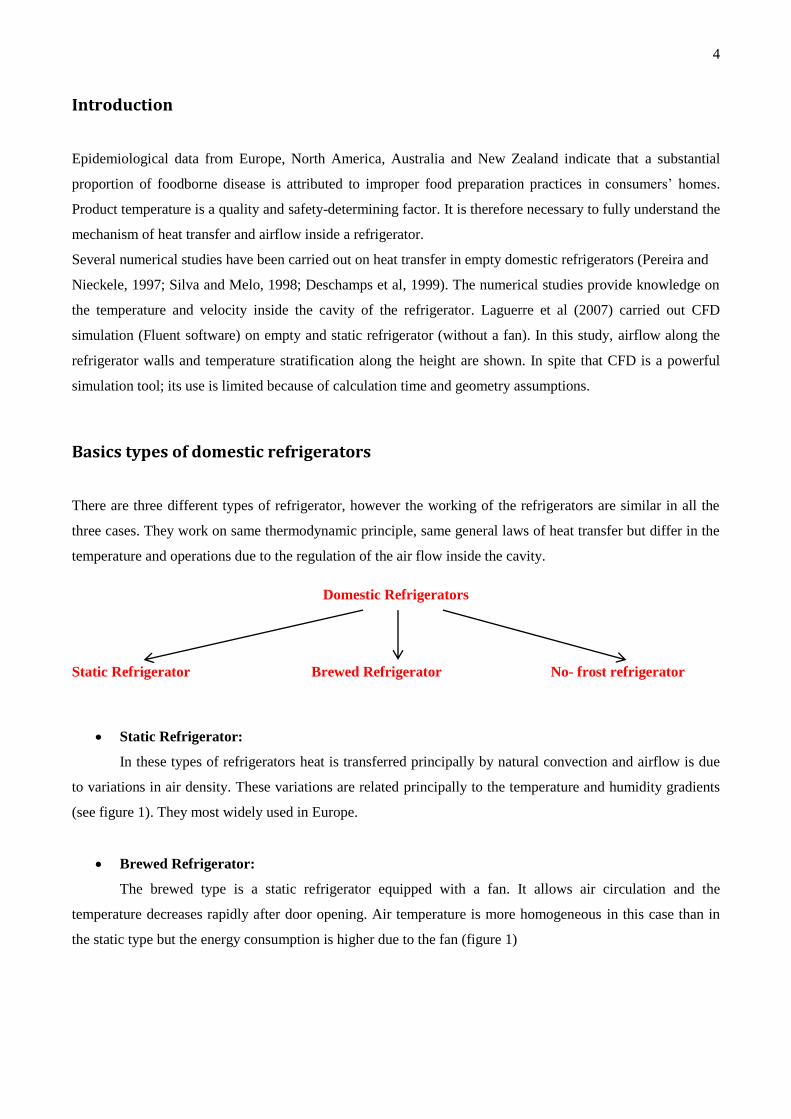
No- frost refrigerator:

In a no-frost refrigerator (figure 1), a fan (embedded in the back wall) pushes air to flow over the

evaporator before entering into the refrigerating compartment. Air temperature is more homogeneous

compared to the two other refrigerator types. Disadvantages of no-frost type are noise, energy consumption,

drying on food surface and high price.

Figure 1 a) Static refrigerator b) Brewed Refrigerator c) No Frost refrigerator

Literature Review:

There has been very few or limited studies conducted on the study of the air recirculation inside refrigerators

due to the complexity of scientific study of measurement. However very limited edition of the study of the air

flow inside a refrigerator by Lacerda et al (Sergelidis, 1995) using PIV technology was mainly influenced by

the on & off cycles of the compressor. The factors that played a great role were the natural convection of the

heat transfer and the dependency of the air viscosity. Air flow inside a refrigerator cavity is mainly influenced

by the aspect ratio of the refrigerator i.e. the ratio of height to the width (Laguerre, 2008).

To understand the implications of the natural convection and air flow couple of illustrations are represented

below having some common configurations of cold vertical plate with an air flow & air flow in empty closed

cavity and heat transfer.

6

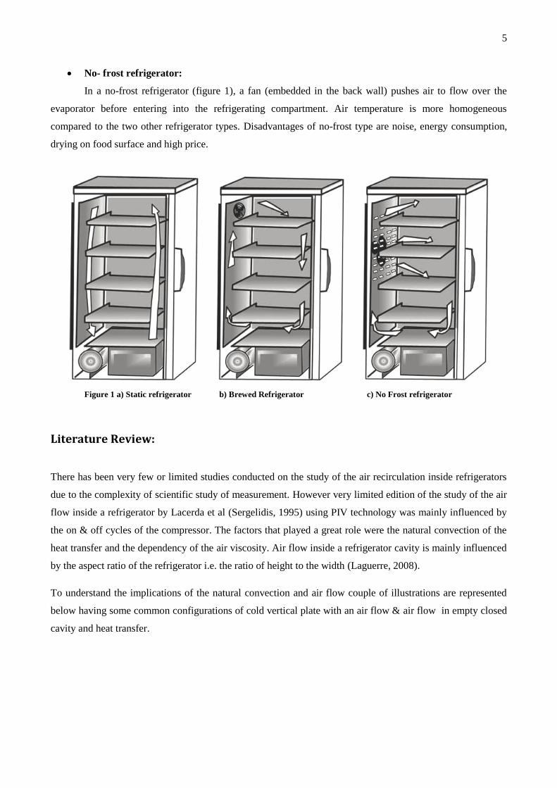
Airflow near a Vertical Plate:

The flow is best understood when a vertical cold plate is placed in the warm region (without limiting walls on

the either side). The convection will ease the understanding of the airflow by natural convection that occurs

near the evaporator of the refrigerator. If a tracer is induced in the flow, it gives a more effective

understanding. It shows a laminar flow near the wall but as moved further from the wall turbulent region can

be seen.

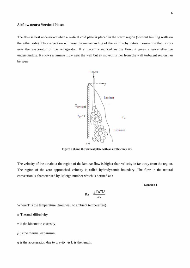
The velocity of the air about the region of the laminar flow is higher than velocity in far away from the region.

The region of the zero approached velocity is called hydrodynamic boundary. The flow in the natural

convection is characterised by Raleigh number which is defined as :

Equation 1

Ra =𝑔𝛽∆TL3

𝛼v

Where T is the temperature (from wall to ambient temperature)

𝛼 Thermal diffusivity

v is the kinematic viscosity

𝛽 is the thermal expansion

g is the acceleration due to gravity & L is the length.

Figure 2 shows the vertical plate with an air flow in y axis

7

Figure 3 shows the boundary layer and the velocity profile in natural convection

Air Flow in empty closed cavity and heat transfer:

Air recirculation inside a closed cavity of the refrigerator completely depends upon the aspect ratio of the

cavity and the temperature difference between the walls of the flow regime. Experimental studies from

Ostrach () & Yang () showed when the bottom horizontal wall is cold, stable temperature difference is

obtained. When the upper horizontal wall is cold there is an unstable distribution of the air inside the

refrigerator due to the effect of gravity. While having the side walls as the colder region shows a stagnation of

cold air around the wall and hotter air at the centre. .

Air Flow recirculation in a refrigerator

Air recirculation inside a refrigerator plays an important role in keeping the consumables fresh and healthy.

Since it needs to keep a constant temperature inside the cavity, the temperature needs to be uniformly

distributed. Air is the ultimate fluid which is used as source to keep the consumables cold. Hence airflow

plays a crucial role in determining the efficiency and cooling of the refrigerators.

Basic of airflow:

Whenever an air flows it generates a resistance. This resistance results into two different forms of flows:

8

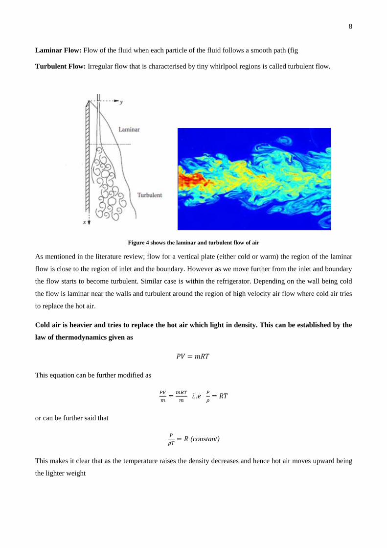
Laminar Flow: Flow of the fluid when each particle of the fluid follows a smooth path (fig

Turbulent Flow: Irregular flow that is characterised by tiny whirlpool regions is called turbulent flow.

Figure 4 shows the laminar and turbulent flow of air

As mentioned in the literature review; flow for a vertical plate (either cold or warm) the region of the laminar

flow is close to the region of inlet and the boundary. However as we move further from the inlet and boundary

the flow starts to become turbulent. Similar case is within the refrigerator. Depending on the wall being cold

the flow is laminar near the walls and turbulent around the region of high velocity air flow where cold air tries

to replace the hot air.

Cold air is heavier and tries to replace the hot air which light in density. This can be established by the

law of thermodynamics given as

𝑃𝑉 = 𝑚𝑅𝑇

This equation can be further modified as

𝑃𝑉

𝑚=

𝑚𝑅𝑇

𝑚 i..e

𝑃

𝜌= 𝑅𝑇

or can be further said that

𝑃

𝜌𝑇= 𝑅 (constant)

This makes it clear that as the temperature raises the density decreases and hence hot air moves upward being

the lighter weight

9

Relation of heat and airflow in a refrigerator

As the equation 𝑃

𝜌𝑇= 𝑅 states that warm air rises up and cold air replaces being heavily dense, this generates

circular airflow in the cavity & temperature stratification along the height.

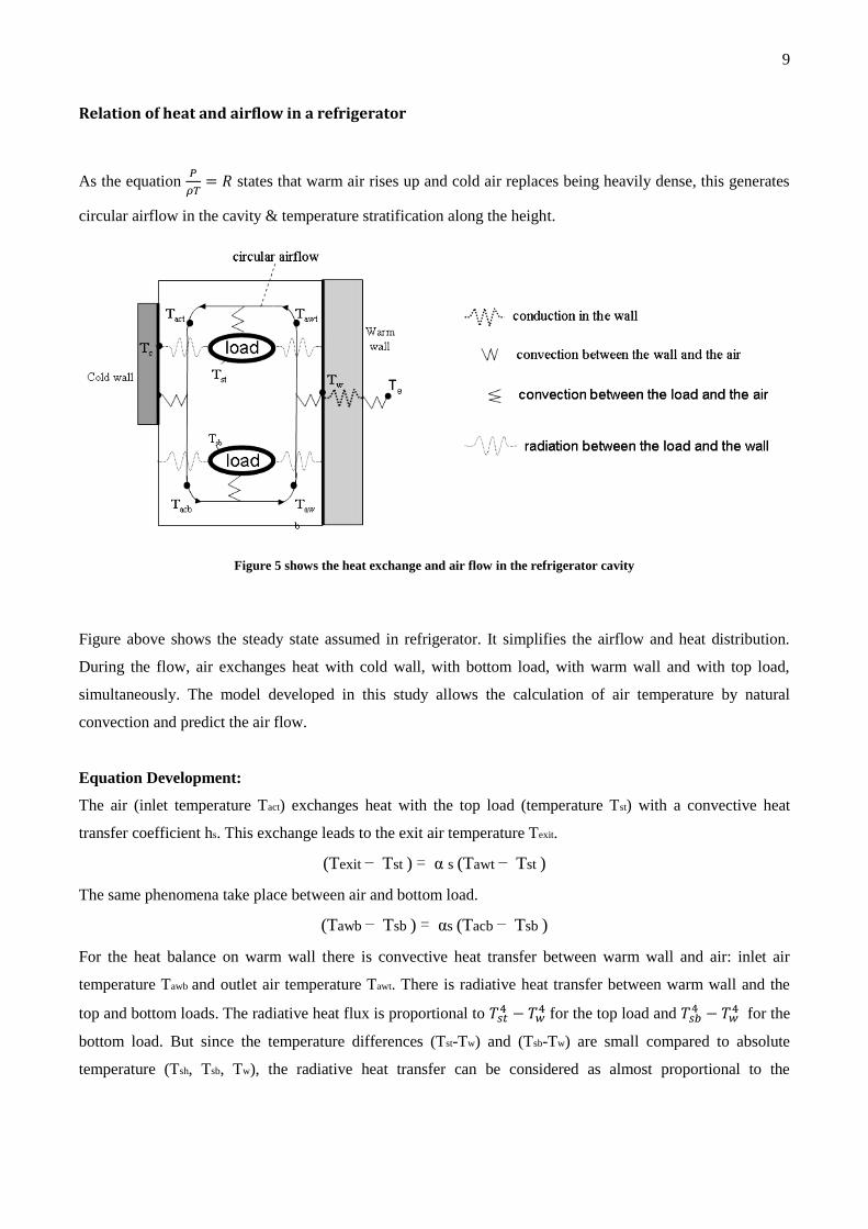
Figure 5 shows the heat exchange and air flow in the refrigerator cavity

Figure above shows the steady state assumed in refrigerator. It simplifies the airflow and heat distribution.

During the flow, air exchanges heat with cold wall, with bottom load, with warm wall and with top load,

simultaneously. The model developed in this study allows the calculation of air temperature by natural

convection and predict the air flow.

Equation Development:

The air (inlet temperature Tact) exchanges heat with the top load (temperature Tst) with a convective heat

transfer coefficient hs. This exchange leads to the exit air temperature Texit.

(Texit − Tst ) = α s (Tawt − Tst )

The same phenomena take place between air and bottom load.

(Tawb − Tsb ) = αs (Tacb − Tsb )

For the heat balance on warm wall there is convective heat transfer between warm wall and air: inlet air

temperature Tawb and outlet air temperature Tawt. There is radiative heat transfer between warm wall and the

top and bottom loads. The radiative heat flux is proportional to 𝑇𝑠𝑡4 − 𝑇𝑤

4 for the top load and 𝑇𝑠𝑏4 − 𝑇𝑤

4 for the

bottom load. But since the temperature differences (Tst-Tw) and (Tsb-Tw) are small compared to absolute

temperature (Tsh, Tsb, Tw), the radiative heat transfer can be considered as almost proportional to the

10

temperature differences. In steady state, the convective and radiative heat fluxes on the warm wall is balanced

with heat flux from this wall to ambience with the coefficient he.

�̇�Cp (Tawb − Tawt ) + hrwtArwt (Tst − Tw ) + hrwbArwb (Tsb − Tw ) = heAe (Tw − Te )

Or (Tawb − Tawt ) + βrwt (Tst − Tw ) + βrwb (Tsb − Tw ) = βe (Tw − Te )

Heat balance on the top load.

There is convective heat exchange between the top load and air and radiative heat exchange between the load

and the cold and warm walls.

�̇�Cp (Tawt − Tact ) + hrctArct (Tc − Tst ) + hrwtArwt (Tw − Tst ) = 0

Or (Tawt − Tact ) + βrct (Tc − Tst ) + βrwt (Tw − Tst ) = 0

Heat balance on the bottom load:

The same phenomena take place on the bottom load.

(Tacb − Tawb ) + βrcb (Tc − Tsb ) + βrwb (Tw − Tsb ) = 0

Experimentally it is supposed that the room temperature (Te) and air temperature near the thermostat (Tth) are

known. Since, the thermostat sensor is generally located at the bottom of the back wall; it is reasonably to

represent Tth by Tacb. The eqns. can be expressed as:

A.T = B.Te + C.Tth

Where A, B and C are matrix of dimensionless coefficients and T is matrix of temperature to be predicted.

Effect of door ajar on airflow and temperature of a refrigerator

When door is opened, hot and humid ambient air mixes with the chamber cold air. That’s why moisture

transfer increases with increasing the number of door opening. The hot and humid surroundings air cool down

and freeze at the freezer temperature. Then double energy is required to make frost and to defrost it again.

Whereas if the number of door opening increase, the convective heat transfer will increase.

Effect of compressor on & off mode on temperature.

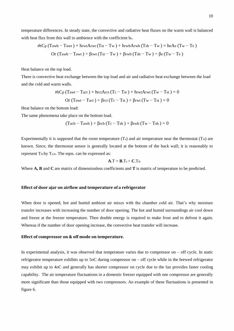
In experimental analysis, it was observed that temperature varies due to compressor on – off cycle. In static

refrigerator temperature exhibits up to 5oC during compressor on – off cycle while in the brewed refrigerator

may exhibit up to 4oC and generally has shorter compressor on cycle due to the fan provides faster cooling

capability. The air temperature fluctuations in a domestic freezer equipped with one compressor are generally

more significant than those equipped with two compressors. An example of these fluctuations is presented in

figure 6.

11

Figure 6 shows temperature fluctuation with in with compressor on - off

Energy loss in refrigerator cavity

Experimental analysis by Alissi et al. found that the presence of door openings caused increases in the daily

energy use of the refrigerator unit by up to 32% over the energy used during a closed door test under the same

ambient conditions. It was also discovered that an increase of 15 of (8 K) in the ambient temperature for an

open door test caused an increase in energy consumption by 44%, and at 70 of, an increase of the relative

humidity from 22% to 91 % caused an increase in the energy consumption by 13%.

The major internal losses include the losses due to the refrigerant irreversible, compression related to the

cylinder inside, the losses due to the refrigerant irreversible decompression in the decompressor, and the

losses of indicated power.

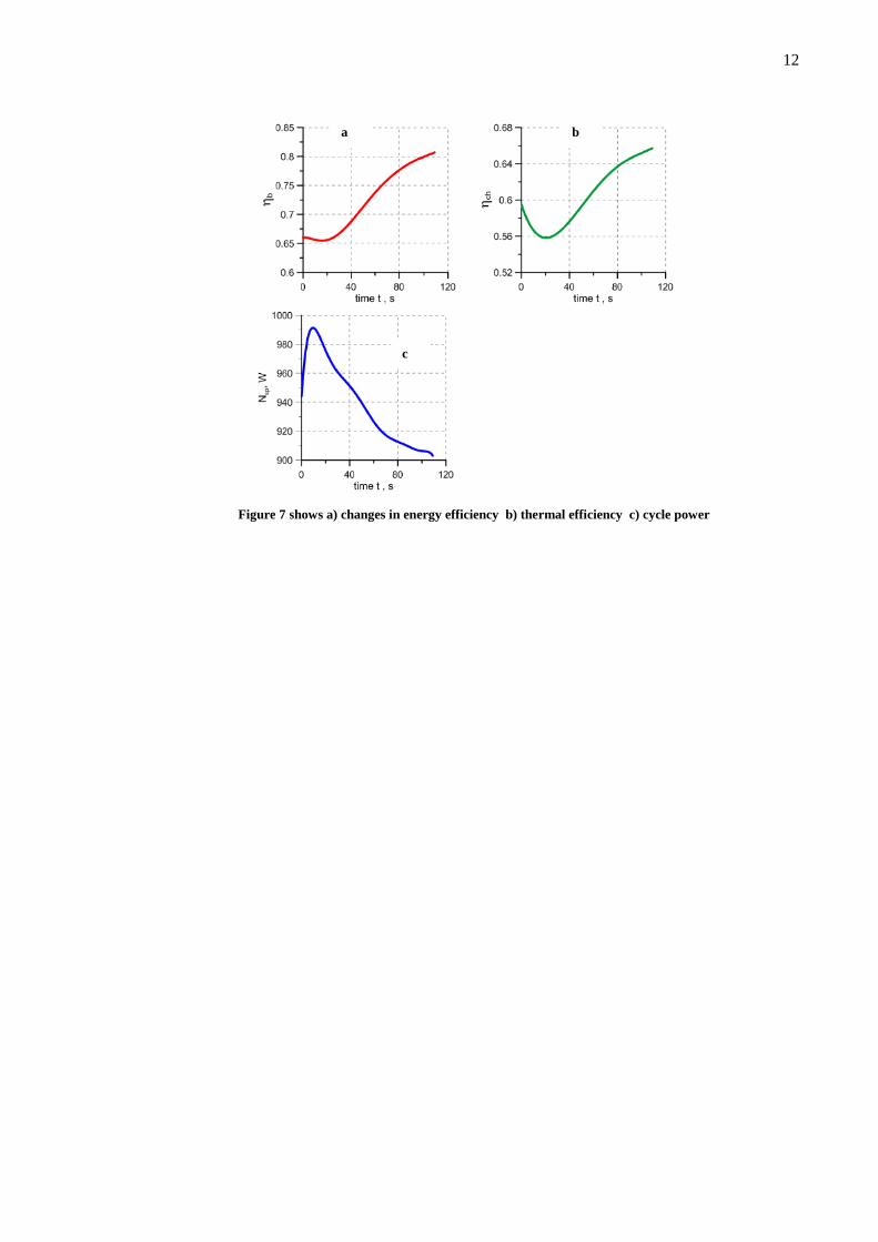
Experimental analysis by Anna Warmińska (Warmińska, 2013) showed the changes in pressure (like opening

the door), temperature and driving power during operation prove that a pressure drop due to a refrigerant flow

through the refrigerator individual elements are inconsiderable and hardly influence energy losses. The largest

energy losses occur during a start-up as shown in the graphs in figure .The examination demonstrated that the

consumption of unit powering energy during a single refrigeration cycle of the immersion refrigerator to

distribute the heat/ temperature and air flow basically depends on refrigerant mass and the use of the

evaporator side. More mass of a refrigerated liquid requires more energy under given circumstances. Any

further increase in unit mass is expected to increase unit energy because of refrigerator limited cooling

efficiency.

12

Figure 7 shows a) changes in energy efficiency b) thermal efficiency c) cycle power

a b

c

13

Methodology - Using Fluent CFD for case study

Pre Processing

Boundary Conditions

Boundary conditions serve the important and most required conditions for the mathematical model (Bakker,

2002). These direct the motion flow of the fluid in the domain.

The inlet & outlet boundary is the condition which serves as the input and output or inlet & outlet of the fluid

flow in the domain. They can be of different types, such as:

For incompressible flows: Velocity inlet and outflow.

General: Pressure inlet and outlet.

For compressible flow: Mass inlet and outlet

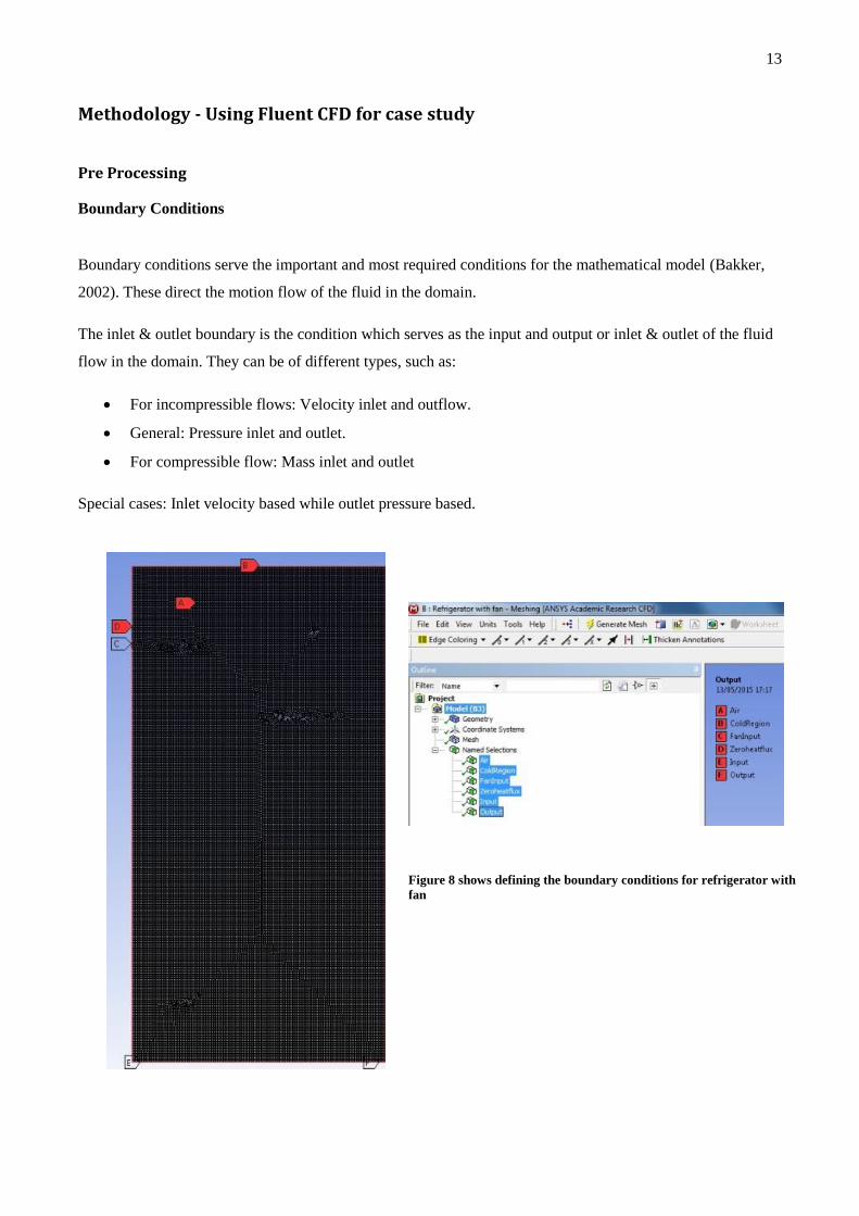
Special cases: Inlet velocity based while outlet pressure based.

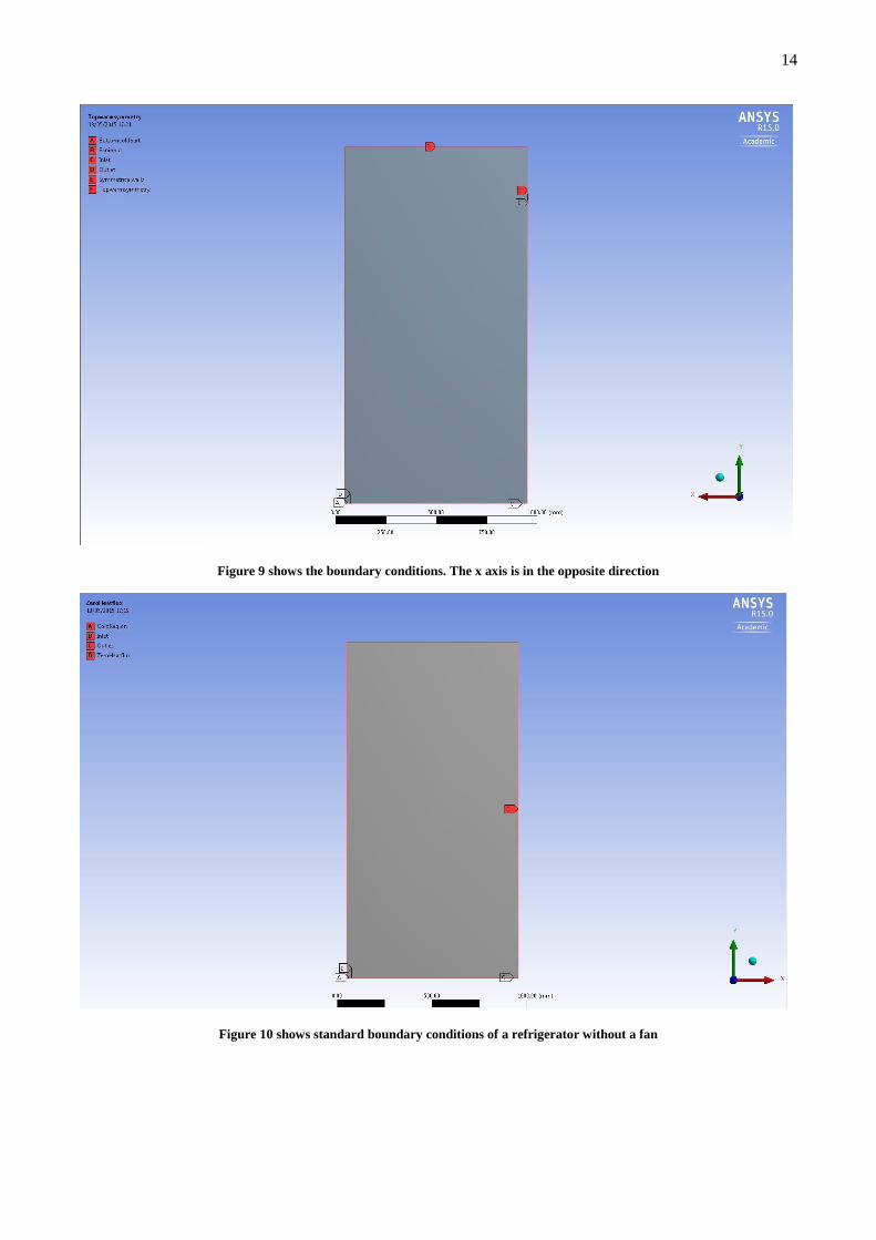
Figure 8 shows defining the boundary conditions for refrigerator with

fan

14

Figure 9 shows the boundary conditions. The x axis is in the opposite direction

Figure 10 shows standard boundary conditions of a refrigerator without a fan

15

Meshing

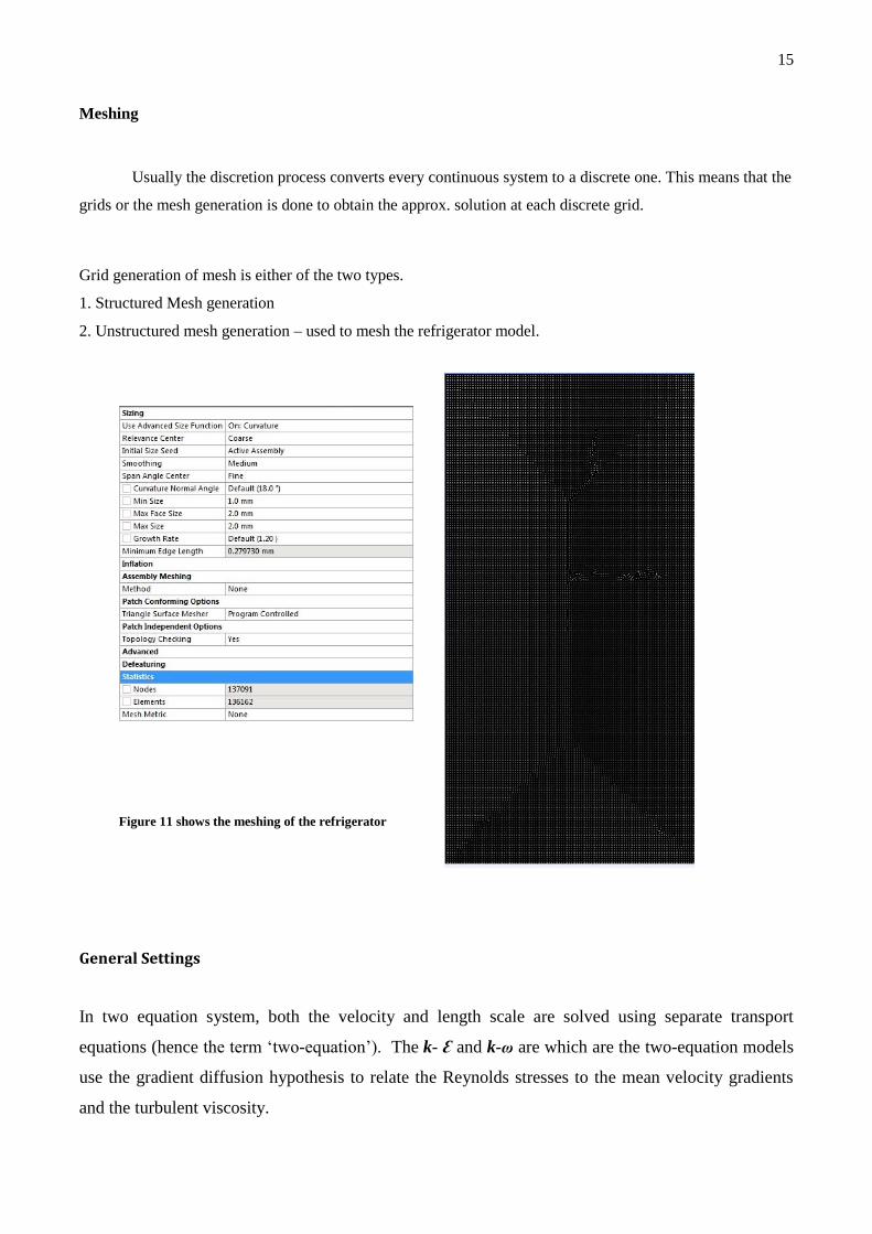
Usually the discretion process converts every continuous system to a discrete one. This means that the

grids or the mesh generation is done to obtain the approx. solution at each discrete grid.

Grid generation of mesh is either of the two types.

1. Structured Mesh generation

2. Unstructured mesh generation – used to mesh the refrigerator model.

General Settings

In two equation system, both the velocity and length scale are solved using separate transport

equations (hence the term ‘two-equation’). The k- Ɛ and k-ω are which are the two-equation models

use the gradient diffusion hypothesis to relate the Reynolds stresses to the mean velocity gradients

and the turbulent viscosity.

Figure 11 shows the meshing of the refrigerator

16

Energy equation

While modelling convective heat transfer we need to switch the energy equation on

Use of gravity

It is important to use the effect of gravity to model the airflow inside the refrigerator. Gravity helps to

underpin the effect of air flow and heat difference while post processing.

Figure 13 shows general settings in the fluent pre processing

Figure 12 shows the processing setup

17

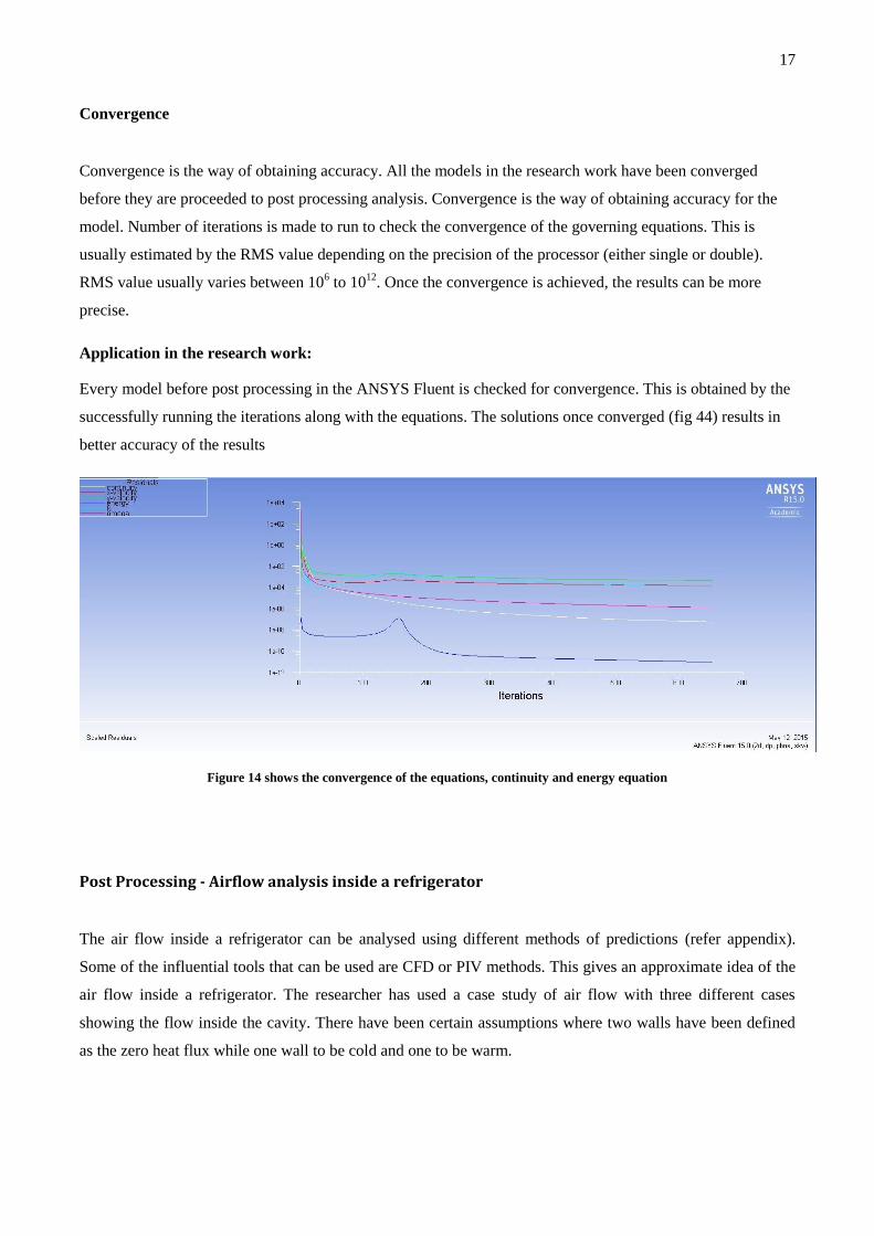
Convergence

Convergence is the way of obtaining accuracy. All the models in the research work have been converged

before they are proceeded to post processing analysis. Convergence is the way of obtaining accuracy for the

model. Number of iterations is made to run to check the convergence of the governing equations. This is

usually estimated by the RMS value depending on the precision of the processor (either single or double).

RMS value usually varies between 106 to 10

12. Once the convergence is achieved, the results can be more

precise.

Application in the research work:

Every model before post processing in the ANSYS Fluent is checked for convergence. This is obtained by the

successfully running the iterations along with the equations. The solutions once converged (fig 44) results in

better accuracy of the results

Figure 14 shows the convergence of the equations, continuity and energy equation

Post Processing - Airflow analysis inside a refrigerator

The air flow inside a refrigerator can be analysed using different methods of predictions (refer appendix).

Some of the influential tools that can be used are CFD or PIV methods. This gives an approximate idea of the

air flow inside a refrigerator. The researcher has used a case study of air flow with three different cases

showing the flow inside the cavity. There have been certain assumptions where two walls have been defined

as the zero heat flux while one wall to be cold and one to be warm.

18

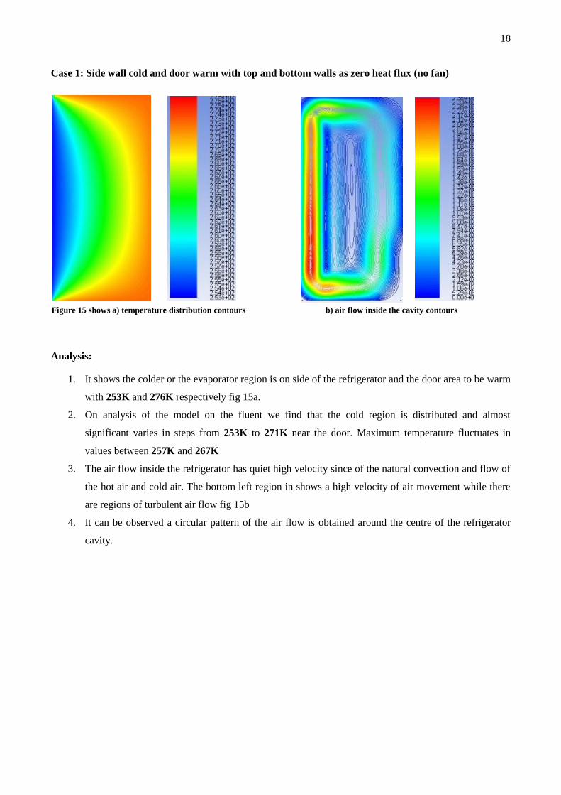
Case 1: Side wall cold and door warm with top and bottom walls as zero heat flux (no fan)

Analysis:

1. It shows the colder or the evaporator region is on side of the refrigerator and the door area to be warm

with 253K and 276K respectively fig 15a.

2. On analysis of the model on the fluent we find that the cold region is distributed and almost

significant varies in steps from 253K to 271K near the door. Maximum temperature fluctuates in

values between 257K and 267K

3. The air flow inside the refrigerator has quiet high velocity since of the natural convection and flow of

the hot air and cold air. The bottom left region in shows a high velocity of air movement while there

are regions of turbulent air flow fig 15b

4. It can be observed a circular pattern of the air flow is obtained around the centre of the refrigerator

cavity.

Figure 15 shows a) temperature distribution contours b) air flow inside the cavity contours

19

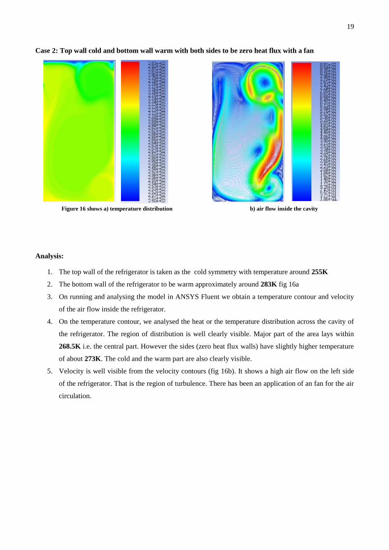
Case 2: Top wall cold and bottom wall warm with both sides to be zero heat flux with a fan

Analysis:

1. The top wall of the refrigerator is taken as the cold symmetry with temperature around 255K

2. The bottom wall of the refrigerator to be warm approximately around 283K fig 16a

3. On running and analysing the model in ANSYS Fluent we obtain a temperature contour and velocity

of the air flow inside the refrigerator.

4. On the temperature contour, we analysed the heat or the temperature distribution across the cavity of

the refrigerator. The region of distribution is well clearly visible. Major part of the area lays within

268.5K i.e. the central part. However the sides (zero heat flux walls) have slightly higher temperature

of about 273K. The cold and the warm part are also clearly visible.

5. Velocity is well visible from the velocity contours (fig 16b). It shows a high air flow on the left side

of the refrigerator. That is the region of turbulence. There has been an application of an fan for the air

circulation.

Figure 16 shows a) temperature distribution b) air flow inside the cavity

20

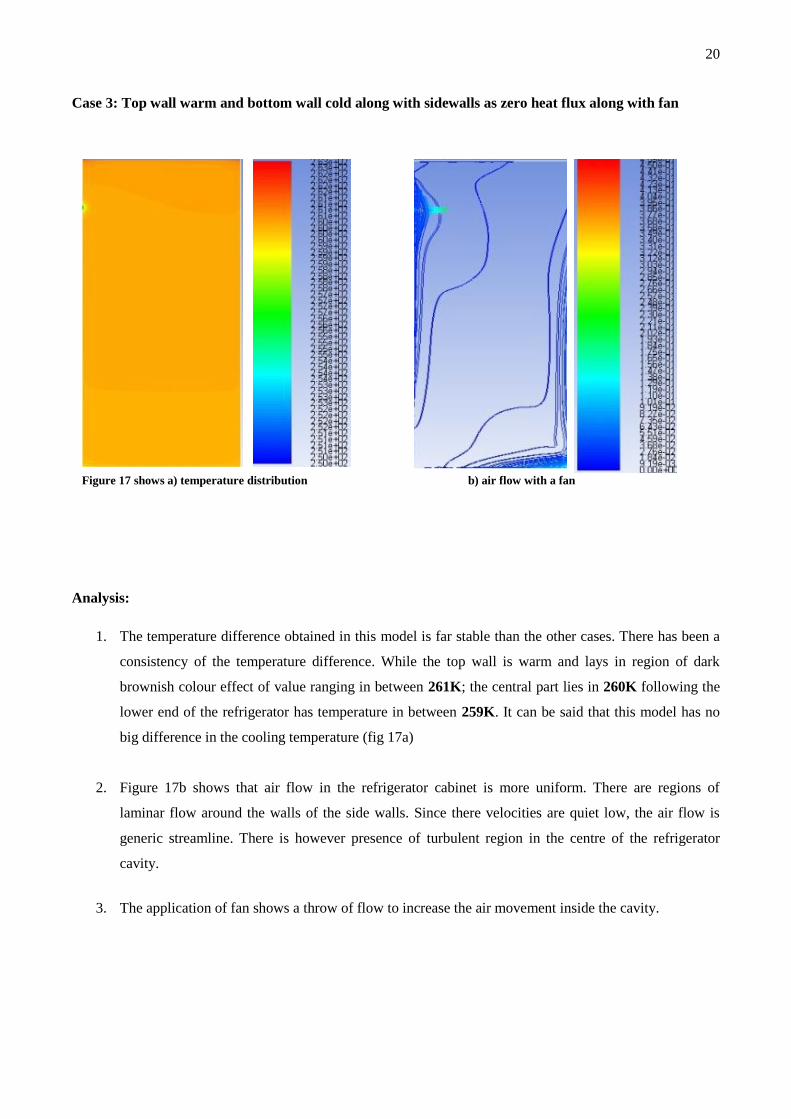
Case 3: Top wall warm and bottom wall cold along with sidewalls as zero heat flux along with fan

Analysis:

1. The temperature difference obtained in this model is far stable than the other cases. There has been a

consistency of the temperature difference. While the top wall is warm and lays in region of dark

brownish colour effect of value ranging in between 261K; the central part lies in 260K following the

lower end of the refrigerator has temperature in between 259K. It can be said that this model has no

big difference in the cooling temperature (fig 17a)

2. Figure 17b shows that air flow in the refrigerator cabinet is more uniform. There are regions of

laminar flow around the walls of the side walls. Since there velocities are quiet low, the air flow is

generic streamline. There is however presence of turbulent region in the centre of the refrigerator

cavity.

3. The application of fan shows a throw of flow to increase the air movement inside the cavity.

Figure 17 shows a) temperature distribution b) air flow with a fan

21

Results & Conclusion:

Heat transfer plays an important role in the air recirculation inside the refrigerator. Air flow inside a

refrigerator cavity can hugely affect the efficiency of the refrigerator. The best practice to have 10% more

efficient cooling is to have the bottom wall cold while the top wall to be warm along with an internal fan. It is

to be reminded that the model was developed based on a given refrigerator design (single door, without a fan).

In future work the model could be used to evaluate the influence of environmental temperatures and operating

conditions on the product temperature evolution along the cold chain (sensitivity study).

22

References

Autodesk Inventor Professional. (2014, March Tuesday ). Autodesk Inventor Help . Retrieved April 16, 2015,

from Autodesk Inventor: http://help.autodesk.com/view/INVNTOR/2014/ENU/?guid=GUID-

B1667D21-A38F-4B20-901B-186EA039DF5A

Bakker, A. (2002). Bakker Organisation. Retrieved April 26, 2015, from Computational Fluid Dynamics:

http://www.bakker.org/dartmouth06/engs150/06-bound.pdf

Clausing, M. R. (1992). Sensible and Latent Energy Loading on a Refrigerator During Open Door

Conditions. Urbana. IL 61801: University of Illinois.

Engineering Tool. (2014, March 20). Retrieved April Tuesday, 2015, from Engineering Tool Box:

http://www.engineeringtoolbox.com/equation-continuity-d_180.html

Laguerre, O. (2008). PIV measurement of the flow field in a domestic refrigerator model: Comparison with

3D simulations. international journal of refrigeration, 1-13.

SAS IP. (n.d.). Meshing. Retrieved April 1st, 2015, from ANSYS CFD online:

http://www.arc.vt.edu/ansys_help/flu_ug/flu_ug_mesh_quality.html

Sergelidis, D. (1995). Temperature distribution and prevalence of Listeria spp. in domestic, retail and

industrial refrigerators in Greece. International Journal of food microbiology, 2-3.

Wakley, J. (2006). Mesh Quality of a three dimensional finite element solutions on anisotropic materials.

Leeds: University of Leeds.

Warmińska, A. (2013). Energy Losses in the Immersion Compression Refrigerator. Lubiin : Politechnika

Lubelska.

Kuzmin, D. (2013). Introduction to Computational Fluid Dynamics. Dortmud: Institute of Applied

Mathematic, University of Dortmud

23

Appendix

NAVIER STOKES EQUATION

The Navier Stokes equation provides the foundation for fluids in motion. It is one more important

topic along with equation of continuity. It is important to discuss Navier Stokes equation as it forms the base

of the analysis if the fluid flows in CFD. Fluid has no limits for distortion when forces are applied. This means

that the fluid goes through number of forces. To simplify Navier derived an equation for the viscous fluid

Stokes slightly modified the equation to form a basic equation called Navier-Stokes equation:

The easy way to remember Navier Stokes equation is by understanding the concept1. The whole process is

categorised into following three sections:

Transient

Convection

Diffusion.

Transient: It refers to the rate of change of the quantity in an infinite volume for a temporary time. Assuming

φ is any random physical quantity like mass, pressure, density, temperature or any other factor. Hence

mathematically transient process can be defined as

𝜕𝜌φ

𝜕𝑡

Convection: If there is any presence of the velocity within the field, the quantity is transported. This is

defined as the convection method and is the first derivative multiplied by the velocity. Mathematically

represented as

𝛻. (𝝆𝒖𝛗)

Diffusion: It refers to the transport of the quantity due to the presence of gradients of that quantity. It is

referred in the mathematical terms as

𝛻. λ𝛻𝛗

Where λ refers to the diffusion constant. This is equal to the thermal conductivity in the heat transfer.

Finally all the three equations are combined to obtain an accumulated equation referred to general transport

equation shown as

. Transient + Convection = Diffusion + Source

1 Shown in Patankar’s brief for understanding Navier Stokes Equation.

24

𝜕𝜌φ

𝜕𝑡+ 𝛻. (𝝆𝒖𝛗) = 𝛻. λ𝛻𝛗 + 𝑆𝑜𝑢𝑟𝑐𝑒𝛗

When obtaining the equation of continuity it can be said that 𝛗 is 1 (for compressible flows). When the

diffusion is not present and absence of the source all the terms can be set to 0.

𝜕𝜌

𝜕𝑡+ 𝛻. (𝝆𝒖) = 0

To obtain the Navier Stokes equation the physical factor φ can be replaced by the velocity component at the

time t. This represents the Navier Stokes equation as:

𝜕𝜌𝑢

𝜕𝑡+ 𝛻. (𝝆𝒖𝑢) = 𝛻. 𝜇𝛻𝑢 −

𝜕𝜌

𝜕𝑥+ 𝜌𝑔𝑥 Equation 12

Similarly in the equation if u is replaced by v and w for y and z coordinates’.

CONTINUTY EQUATION

According to the law of conservation, it can be stated that the mass can neither be created nor be destroyed.

This law can be used in the steady flow process which means that there is no change in the flow rate with time

through a control volume when the stored mass of the control does not change. (Engineering Tool, 2014)

This means inflow is equal to the outflow.

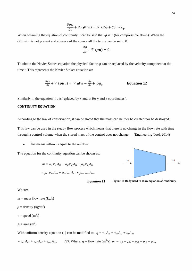
The equation for the continuity equation can be shown as:

m = ρi1 vi1 Ai1 + ρi2 vi2 Ai2 + ρin vin Aim

= ρo1 vo1 Ao1 + ρo2 vo2 Ao2 + ρom vom Aom

Equation 11

Where:

m = mass flow rate (kg/s)

ρ = density (kg/m3)

v = speed (m/s)

A = area (m2)

With uniform density equation (1) can be modified to : q = vi1 Ai1 + vi2 Ai2 +vin Aim

= vo1 Ao1 + vo2 Ao2 + vom Aom (2); Where: q = flow rate (m3/s) ρi1 = ρi2 = ρin = ρo1 = ρo2 = ρom

Figure 18 Body used to show equation of continuity