Embed Size (px)
Citation preview
Convolution Neural Network
By-Amit Kushwaha
• The basic learning entity in the network - Perceptron
•Important Aspects of Deep Learning
Presentation Covers

Machine Learning Engineer @
Who am I
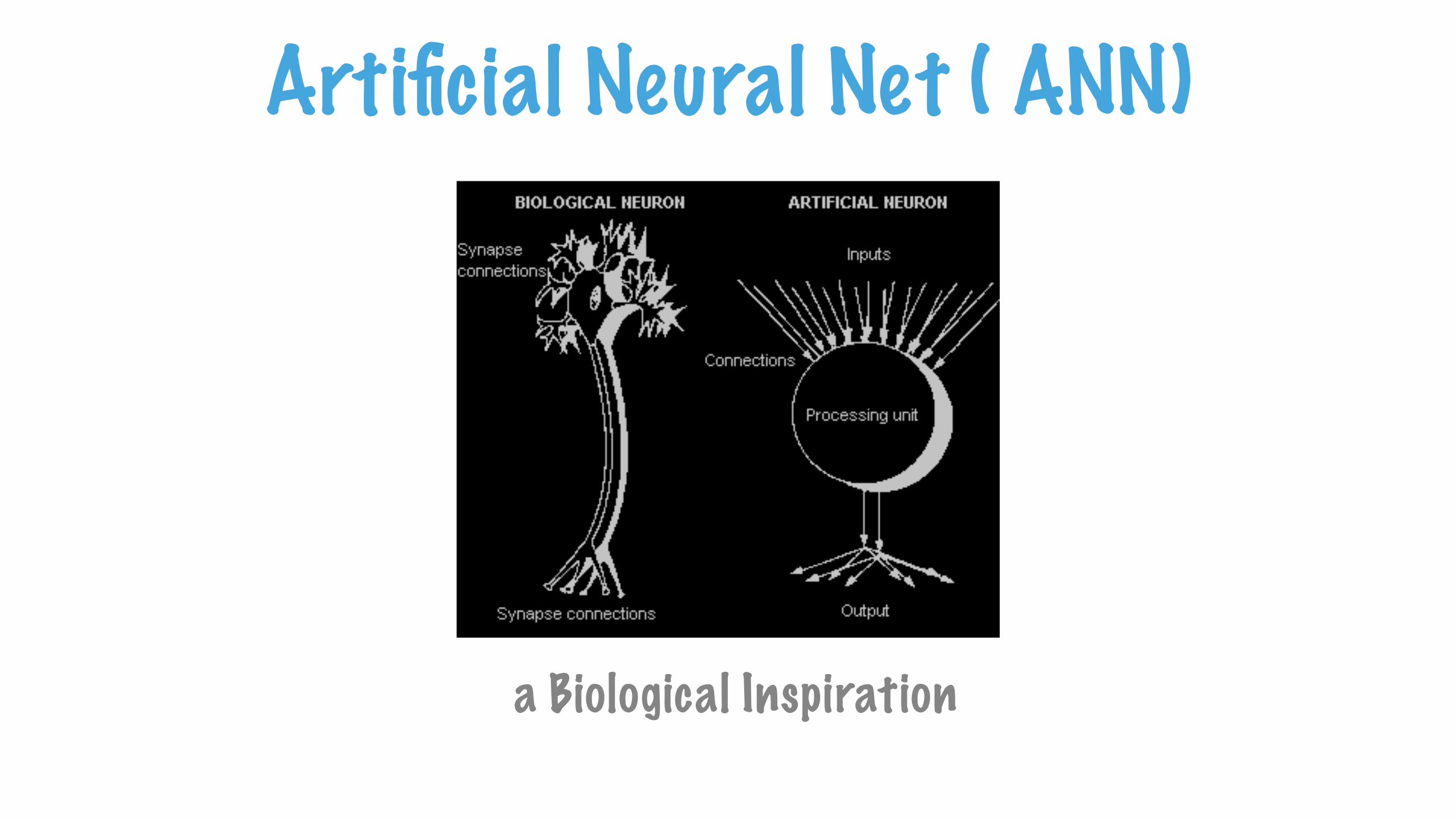
a Biological Inspiration
Artificial Neural Net ( ANN)
The most basic form of neural network which can also learn
Perceptron
The elementary entity of a neural network.
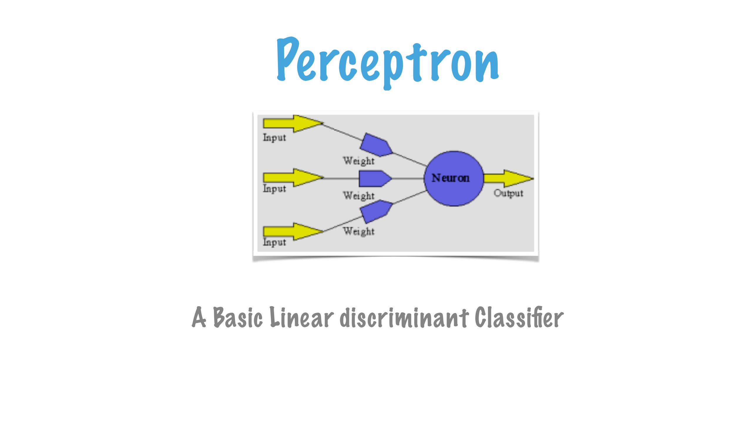
Perceptron
A Basic Linear discriminant Classifier
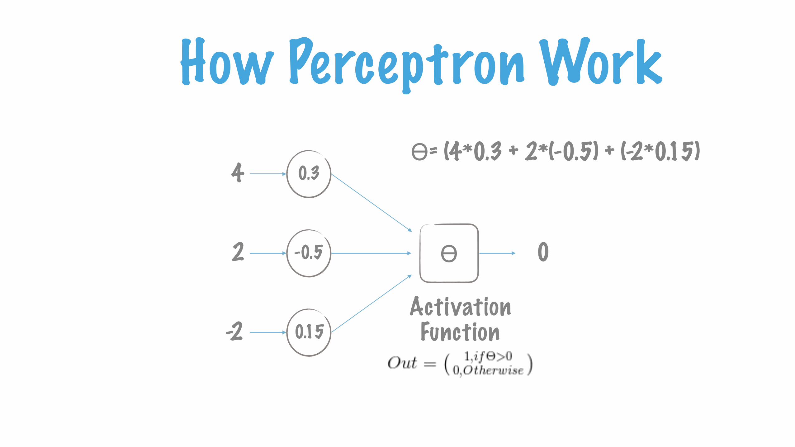
How Perceptron Work0.3
-0.5
0.15Activation Function
ϴ
4
2
-2
0
ϴ= (4*0.3 + 2*(-0.5) + (-2*0.15)
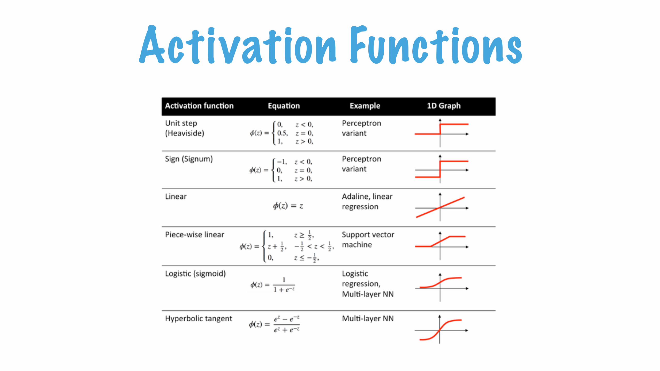
Activation Functions
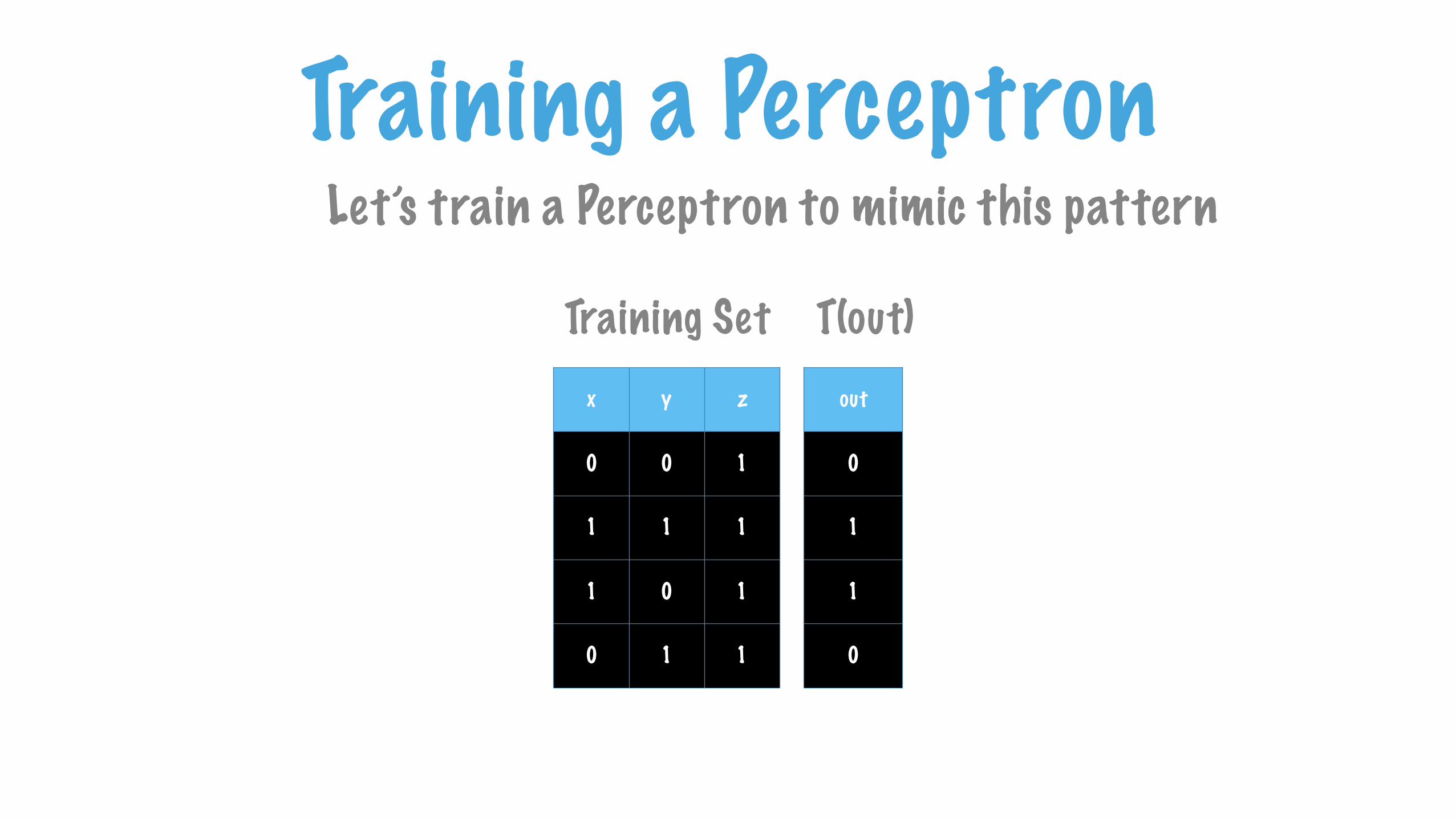
Training a PerceptronLet’s train a Perceptron to mimic this pattern
x y z
0 0 1
1 1 1
1 0 1
0 1 1
Training Setout
0
1
1
0
T(out)

Training a PerceptronPerceptron Model
W1
w4Activation Function
ϴ OutPutW2
W3
x
y
z
1

Wi = Wi + ∆Wi ∆W = -η * ( target output - perceptron output)*X
η is learning rate for perceptron
Training Rules :
W1
w4Activation Function
ϴ OutPutW2
W3
x
y
z
1
Training a Perceptron
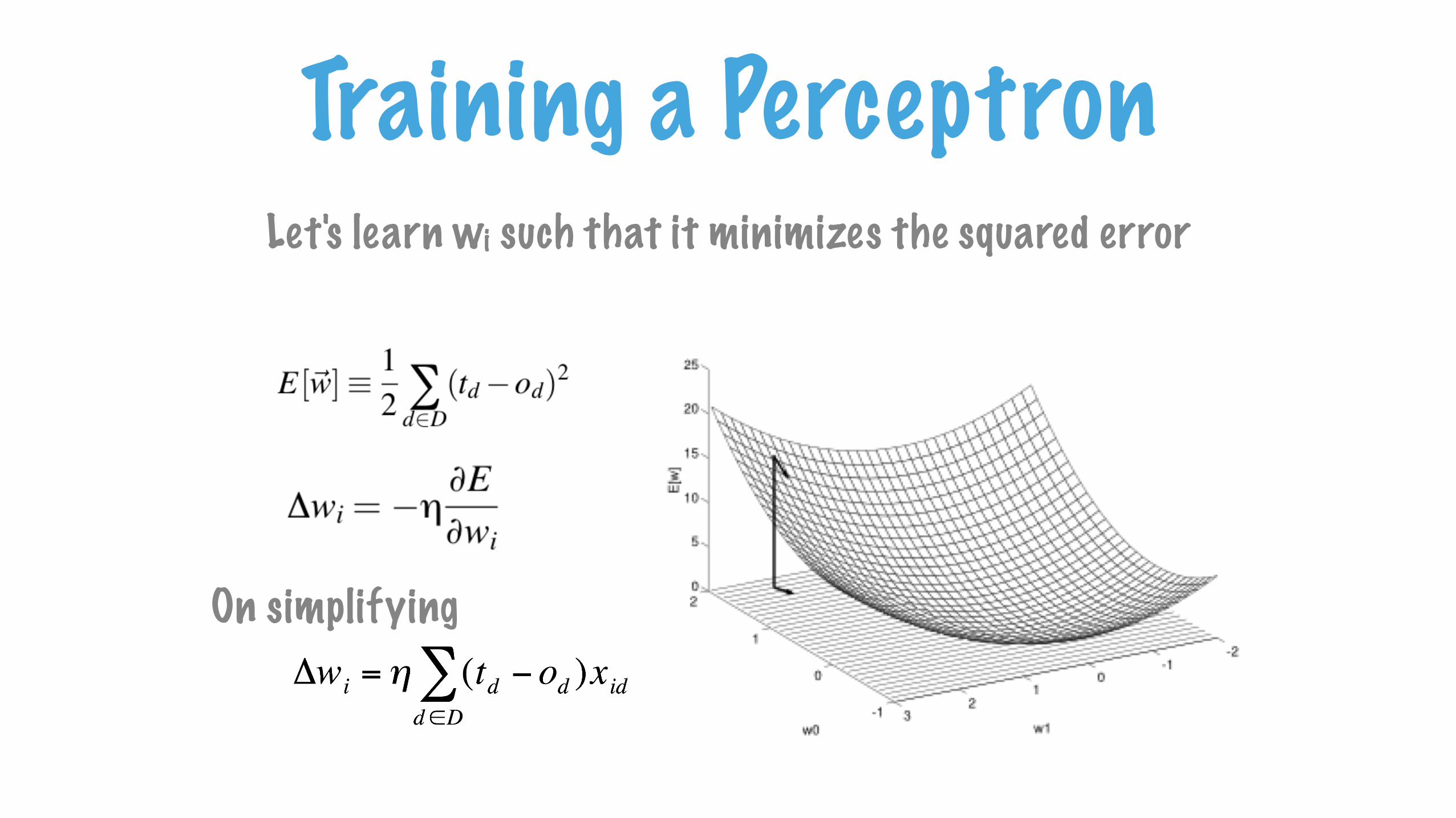
Let's learn wi such that it minimizes the squared error
On simplifying
Training a Perceptron

W1
ϴ Out
Assign random values to Weight Vector([W1,W2,W3,W4])
x y z bias0 0 1 11 1 1 11 0 1 10 1 1 10 0 1 11 1 1 11 0 1 10 1 1 1
Training Setout01100110
T(out)
W2
W3
W4
x
y
z
bias
{{
epoch 1
epoch 2
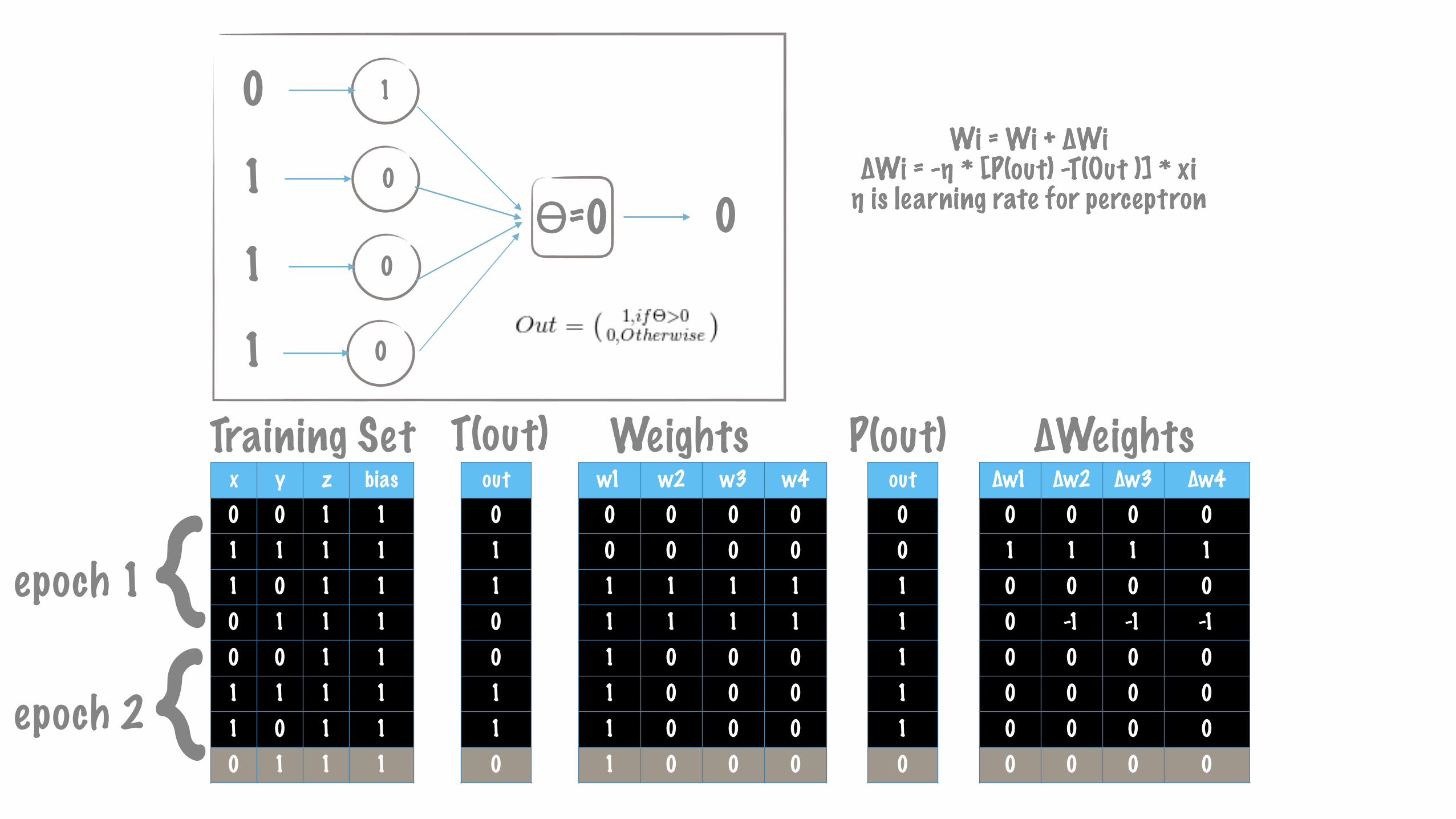
Wi = Wi + ∆Wi ∆Wi = -η * [P(out) -T(Out )] * xi η is learning rate for perceptron
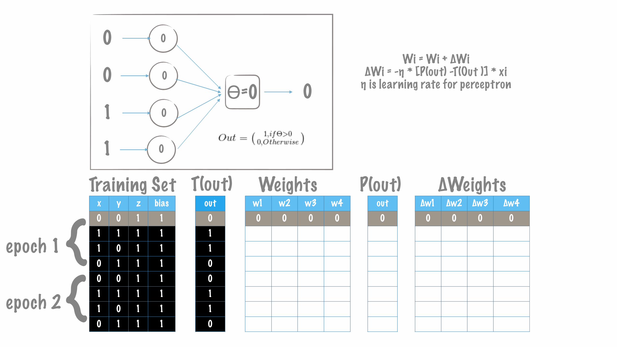
x y z bias0 0 1 11 1 1 11 0 1 10 1 1 10 0 1 11 1 1 11 0 1 10 1 1 1
∆w1 ∆w2 ∆w3 ∆w40 0 0 01 1 1 10 0 0 00 -1 -1 -10 0 0 00 0 0 00 0 0 00 0 0 0
w1 w2 w3 w40 0 0 00 0 0 01 1 1 11 1 1 11 0 0 01 0 0 01 0 0 01 0 0 0
out00110110
Training Set Weights P(out) ∆Weightsout00110110
T(out)
0
ϴ=0 00
0
0
0
0
1
1
{{
epoch 1
epoch 2
Wi = Wi + ∆Wi ∆Wi = -η * [P(out) -T(Out )] * xi η is learning rate for perceptron
out01100110
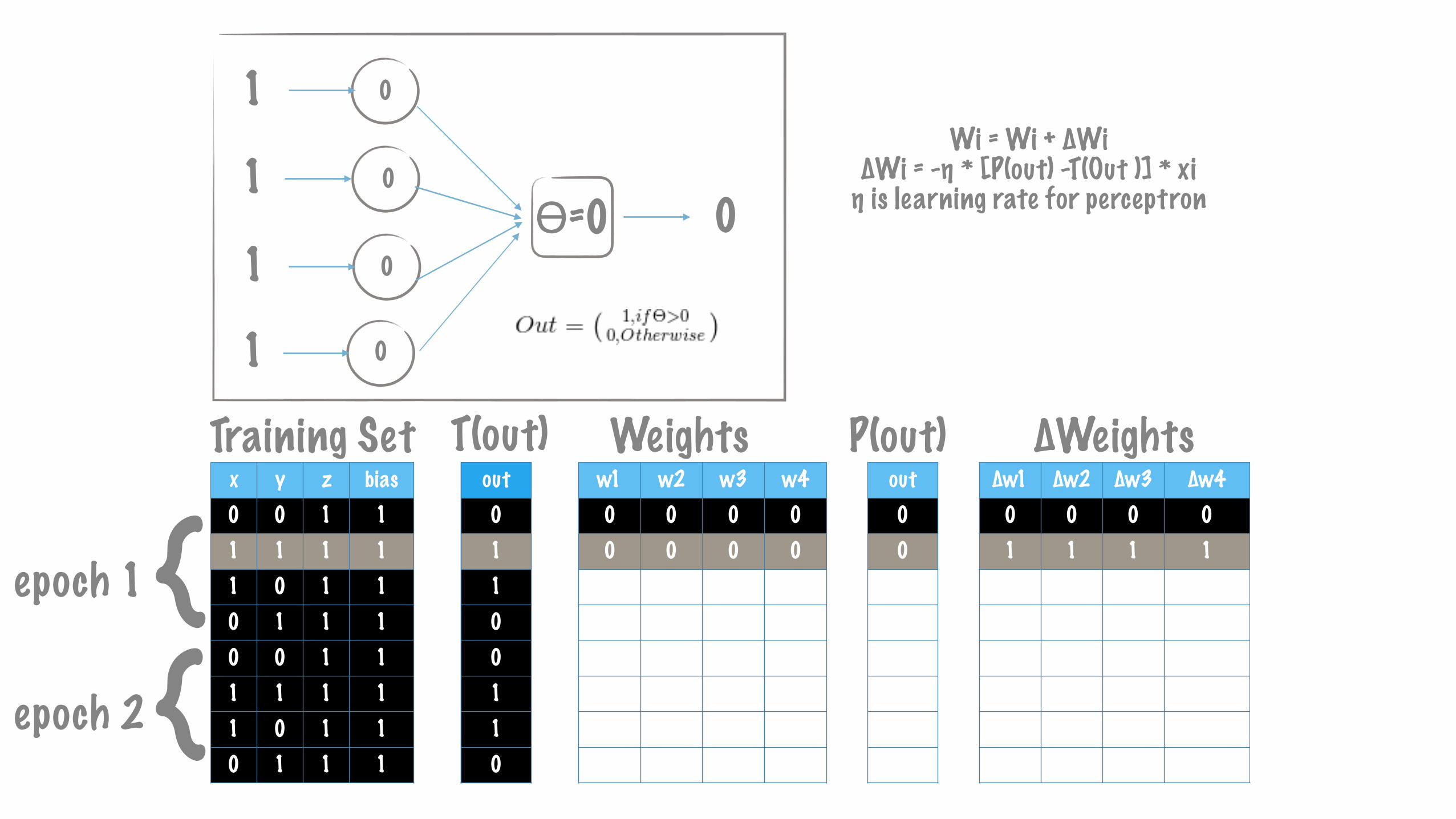
x y z bias0 0 1 11 1 1 11 0 1 10 1 1 10 0 1 11 1 1 11 0 1 10 1 1 1
∆w1 ∆w2 ∆w3 ∆w40 0 0 01 1 1 10 0 0 00 -1 -1 -10 0 0 00 0 0 00 0 0 00 0 0 0
w1 w2 w3 w40 0 0 00 0 0 01 1 1 11 1 1 11 0 0 01 0 0 01 0 0 01 0 0 0
out00110110
Training Set Weights P(out) ∆Weightsout00110110
T(out)
{{
epoch 1
epoch 2
0
ϴ=0 00
0
0
1
1
1
1
Wi = Wi + ∆Wi ∆Wi = -η * [P(out) -T(Out )] * xi η is learning rate for perceptron
out01100110

x y z bias0 0 1 11 1 1 11 0 1 10 1 1 10 0 1 11 1 1 11 0 1 10 1 1 1
∆w1 ∆w2 ∆w3 ∆w40 0 0 01 1 1 10 0 0 00 -1 -1 -10 0 0 00 0 0 00 0 0 00 0 0 0
w1 w2 w3 w40 0 0 00 0 0 01 1 1 11 1 1 11 0 0 01 0 0 01 0 0 01 0 0 0
out00110110
Training Set Weights P(out) ∆WeightsT(out)
{{
epoch 1
epoch 2
0
ϴ=0 00
0
0
1
0
1
1
Wi = Wi + ∆Wi ∆Wi = -η * [P(out) -T(Out )] * xi η is learning rate for perceptron
out01100110

x y z bias0 0 1 11 1 1 11 0 1 10 1 1 10 0 1 11 1 1 11 0 1 10 1 1 1
∆w1 ∆w2 ∆w3 ∆w40 0 0 01 1 1 10 0 0 00 -1 -1 -10 0 0 00 0 0 00 0 0 00 0 0 0
w1 w2 w3 w40 0 0 00 0 0 01 1 1 11 1 1 11 0 0 01 0 0 01 0 0 01 0 0 0
out00110110
Training Set Weights P(out) ∆Weightsout01100110
T(out)
{{
epoch 1
epoch 2
1
ϴ=1 10
1
1
0
1
1
1
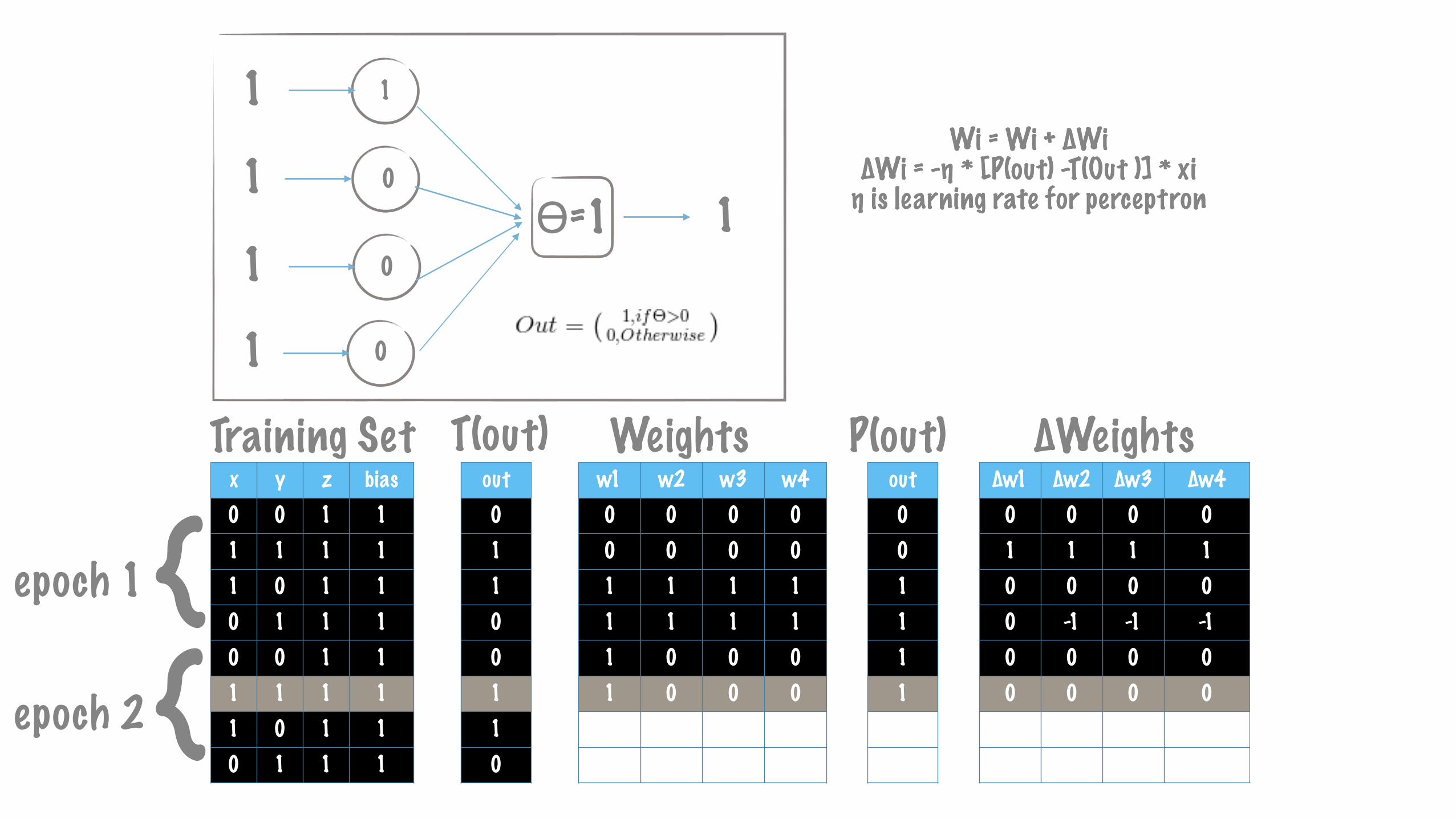
Wi = Wi + ∆Wi ∆Wi = -η * [P(out) -T(Out )] * xi η is learning rate for perceptron

x y z bias0 0 1 11 1 1 11 0 1 10 1 1 10 0 1 11 1 1 11 0 1 10 1 1 1
∆w1 ∆w2 ∆w3 ∆w40 0 0 01 1 1 10 0 0 00 -1 -1 -10 0 0 00 0 0 00 0 0 00 0 0 0
w1 w2 w3 w40 0 0 00 0 0 01 1 1 11 1 1 11 0 0 01 0 0 01 0 0 01 0 0 0
out00110110
Training Set Weights P(out) ∆Weightsout01100110
T(out)
1
ϴ=2 10
1
1
0
0
1
1
Wi = Wi + ∆Wi ∆Wi = -η * [P(out) -T(Out )] * xi η is learning rate for perceptron
{{
epoch 1
epoch 2
Wi = Wi + ∆Wi ∆Wi = -η * [P(out) -T(Out )] * xi η is learning rate for perceptron
x y z bias0 0 1 11 1 1 11 0 1 10 1 1 10 0 1 11 1 1 11 0 1 10 1 1 1
∆w1 ∆w2 ∆w3 ∆w40 0 0 01 1 1 10 0 0 00 -1 -1 -10 0 0 00 0 0 00 0 0 00 0 0 0
w1 w2 w3 w40 0 0 00 0 0 01 1 1 11 1 1 11 0 0 01 0 0 01 0 0 01 0 0 0
out00111110
Training Set Weights P(out) ∆Weightsout01100110
T(out)
1
ϴ=1 10
0
0
1
1
1
1
Wi = Wi + ∆Wi ∆Wi = -η * [P(out) -T(Out )] * xi η is learning rate for perceptron
{{
epoch 1
epoch 2
Wi = Wi + ∆Wi ∆Wi = -η * [P(out) -T(Out )] * xi η is learning rate for perceptron
x y z bias0 0 1 11 1 1 11 0 1 10 1 1 10 0 1 11 1 1 11 0 1 10 1 1 1
∆w1 ∆w2 ∆w3 ∆w40 0 0 01 1 1 10 0 0 00 -1 -1 -10 0 0 00 0 0 00 0 0 00 0 0 0
w1 w2 w3 w40 0 0 00 0 0 01 1 1 11 1 1 11 0 0 01 0 0 01 0 0 01 0 0 0
out00111110
Training Set Weights P(out) ∆Weightsout01100110
T(out)
1
ϴ=1 10
0
0
1
0
1
1
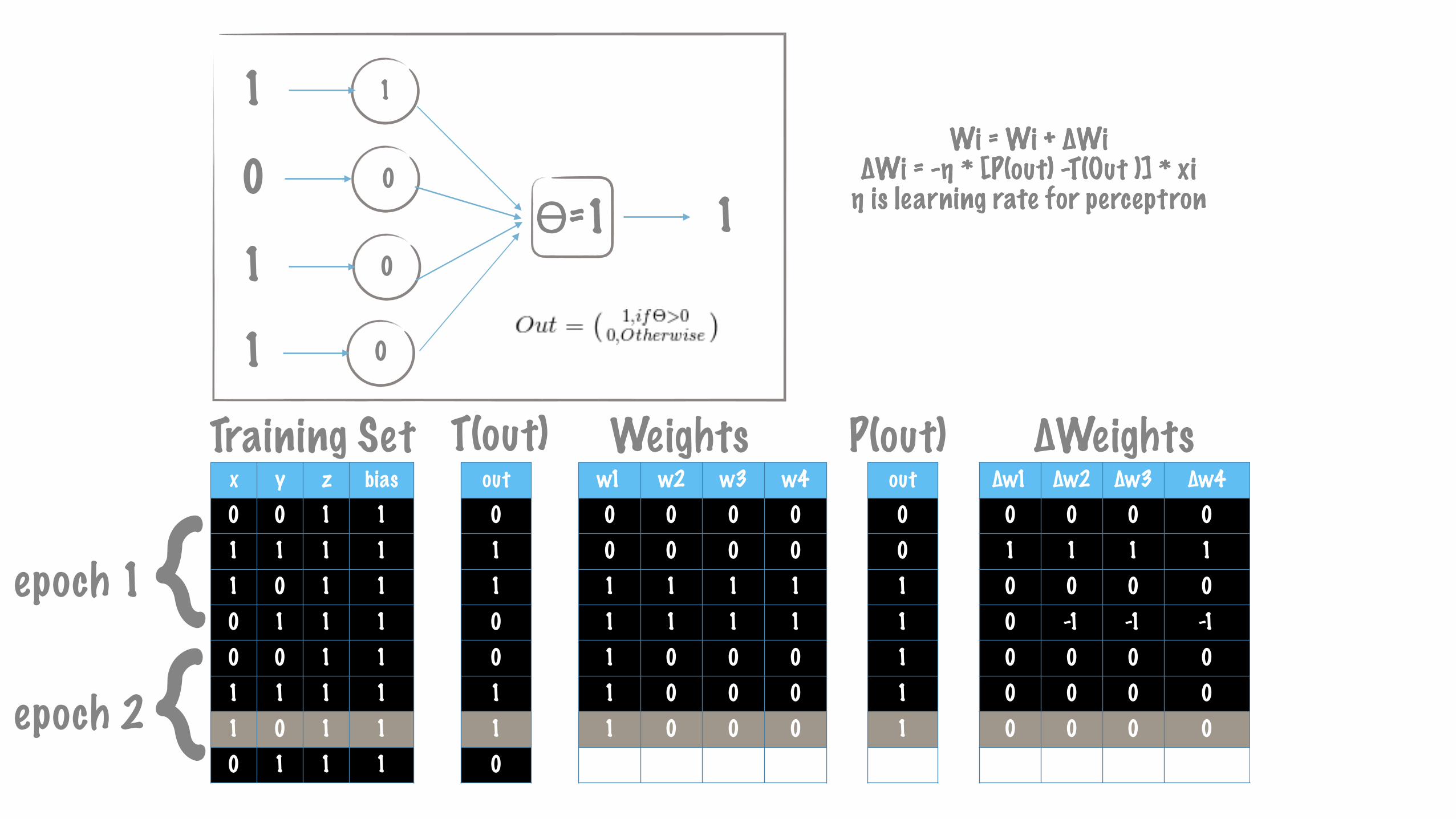
Wi = Wi + ∆Wi ∆Wi = -η * [P(out) -T(Out )] * xi η is learning rate for perceptron
{{
epoch 1
epoch 2
Wi = Wi + ∆Wi ∆Wi = -η * [P(out) -T(Out )] * xi η is learning rate for perceptron
x y z bias0 0 1 11 1 1 11 0 1 10 1 1 10 0 1 11 1 1 11 0 1 10 1 1 1
∆w1 ∆w2 ∆w3 ∆w40 0 0 01 1 1 10 0 0 00 -1 -1 -10 0 0 00 0 0 00 0 0 00 0 0 0
w1 w2 w3 w40 0 0 00 0 0 01 1 1 11 1 1 11 0 0 01 0 0 01 0 0 01 0 0 0
out00111110
Training Set Weights P(out) ∆Weightsout01100110
T(out)
1
ϴ=0 00
0
0
0
1
1
1
Wi = Wi + ∆Wi ∆Wi = -η * [P(out) -T(Out )] * xi η is learning rate for perceptron
{{
epoch 1
epoch 2
Wi = Wi + ∆Wi ∆Wi = -η * [P(out) -T(Out )] * xi η is learning rate for perceptron
x y z bias0 0 1 11 1 1 11 0 1 10 1 1 10 0 1 11 1 1 11 0 1 10 1 1 1
∆w1 ∆w2 ∆w3 ∆w40 0 0 00 0 0 01 0 1 10 0 0 00 0 -1 -10 0 0 00 0 0 00 0 0 0
w1 w2 w3 w41 0 0 00 0 0 00 0 0 01 0 1 11 0 1 11 0 0 01 0 0 01 0 0 0
out00011110
Training Set Weights P(out) ∆Weightsout01100110
T(out)
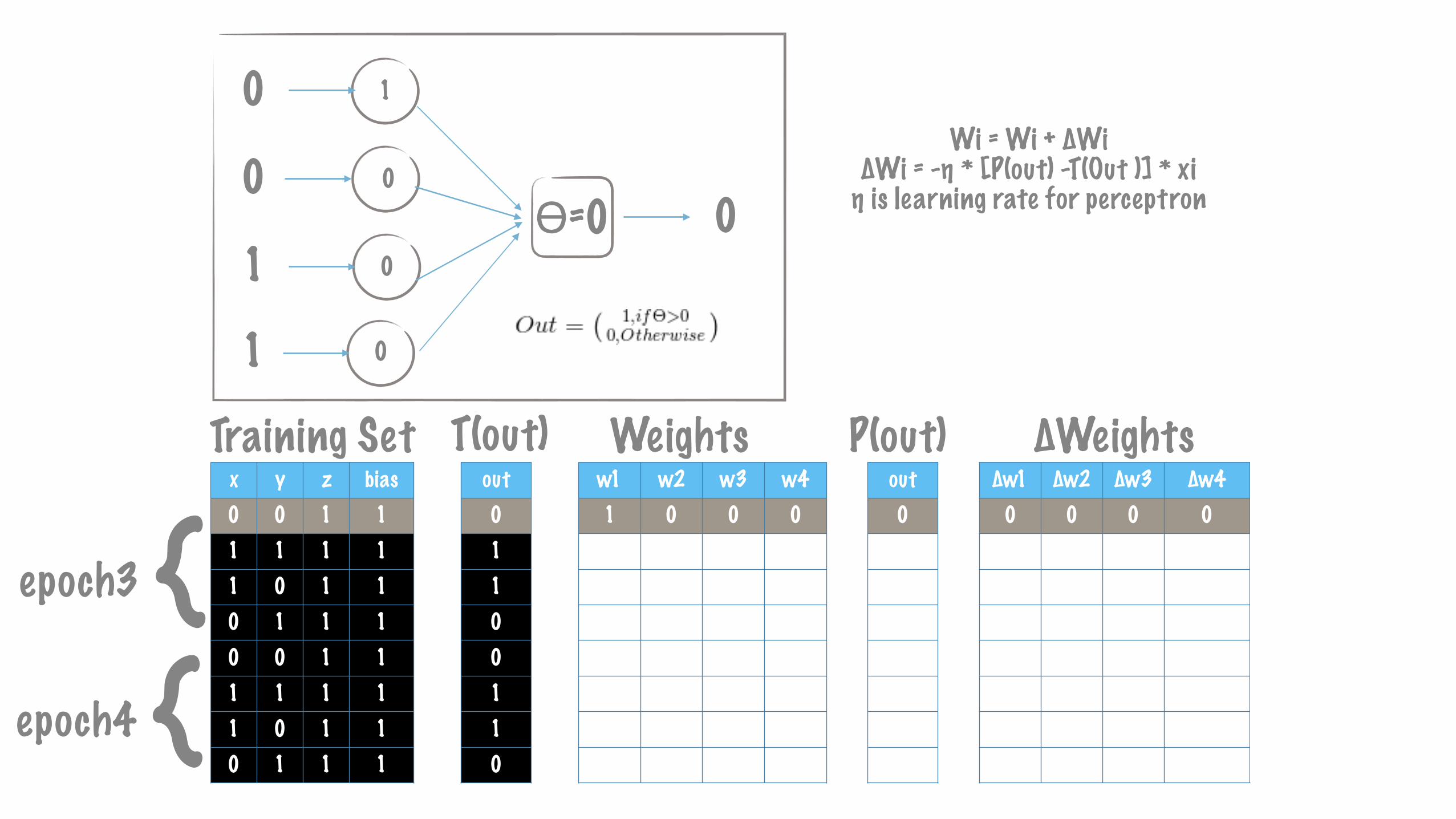
{epoch3
1
ϴ=0 00
0
0
0
0
1
1
Wi = Wi + ∆Wi ∆Wi = -η * [P(out) -T(Out )] * xi η is learning rate for perceptron
{epoch4
x y z bias0 0 1 11 1 1 11 0 1 10 1 1 10 0 1 11 1 1 11 0 1 10 1 1 1
∆w1 ∆w2 ∆w3 ∆w40 0 0 00 0 0 01 0 1 10 0 0 00 0 -1 -10 0 0 00 0 0 00 0 0 0
w1 w2 w3 w41 0 0 01 0 0 00 0 0 01 0 1 11 0 1 11 0 0 01 0 0 01 0 0 0
out01011110
Training Set Weights P(out) ∆Weightsout01100110
T(out)
{epoch3
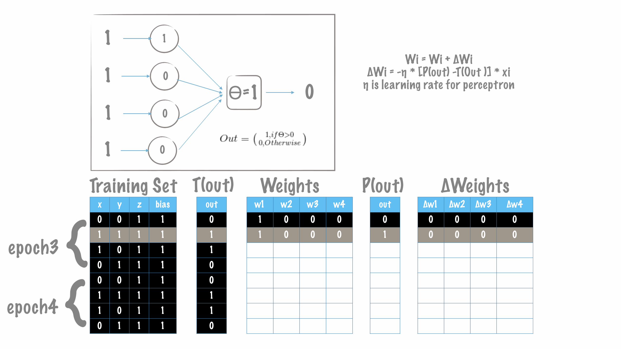
1
ϴ=1 00
0
0
1
1
1
1
Wi = Wi + ∆Wi ∆Wi = -η * [P(out) -T(Out )] * xi η is learning rate for perceptron
{epoch4
x y z bias0 0 1 11 1 1 11 0 1 10 1 1 10 0 1 11 1 1 11 0 1 10 1 1 1
∆w1 ∆w2 ∆w3 ∆w40 0 0 00 0 0 00 0 0 00 0 0 00 0 -1 -10 0 0 00 0 0 00 0 0 0
w1 w2 w3 w41 0 0 01 0 0 01 0 0 01 0 1 11 0 1 11 0 0 01 0 0 01 0 0 0
out01111110
Training Set Weights P(out) ∆Weightsout01100110
T(out)
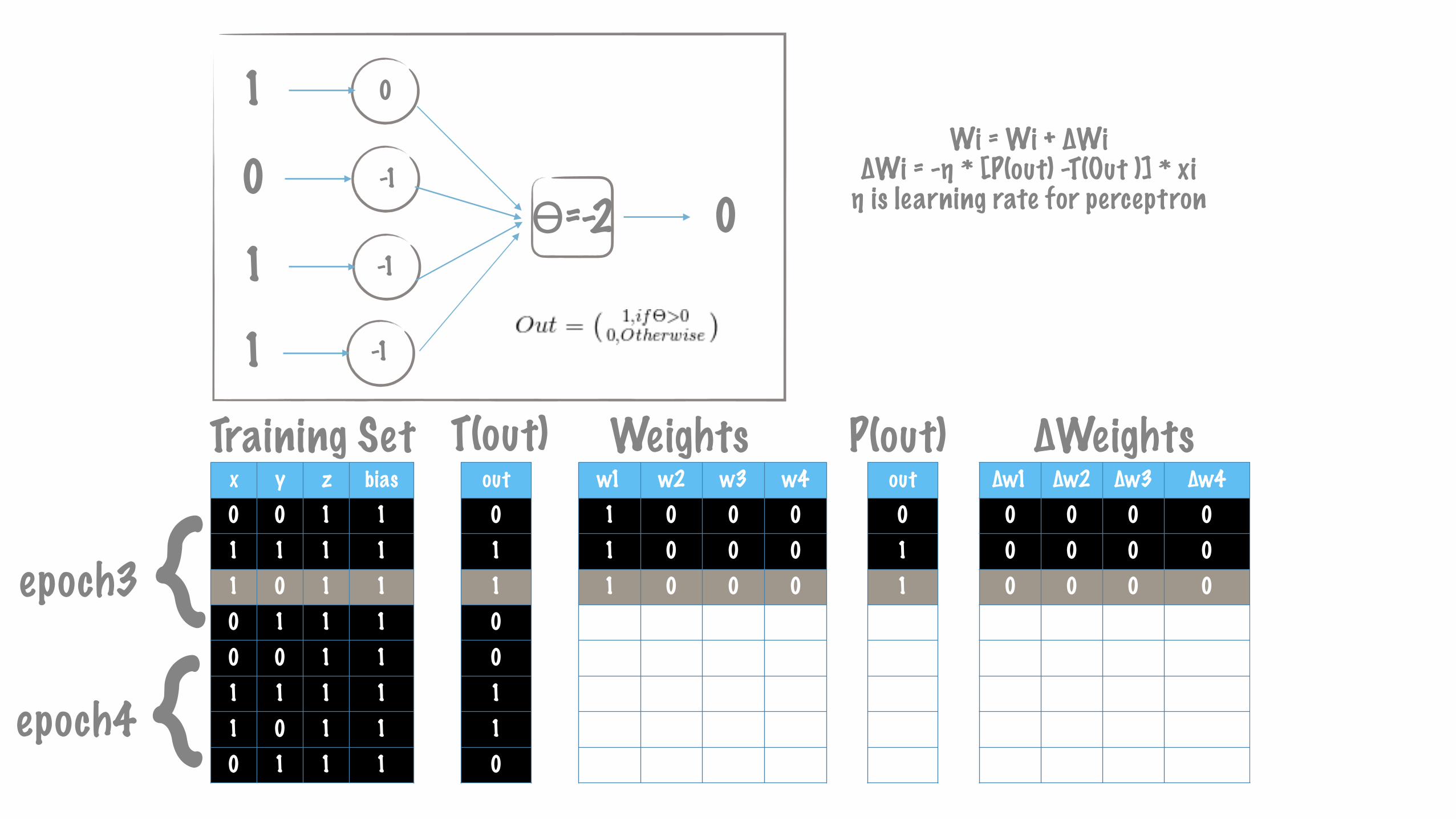
{epoch3
0
ϴ=-2 0-1
-1
-1
1
0
1
1
Wi = Wi + ∆Wi ∆Wi = -η * [P(out) -T(Out )] * xi η is learning rate for perceptron
{epoch4
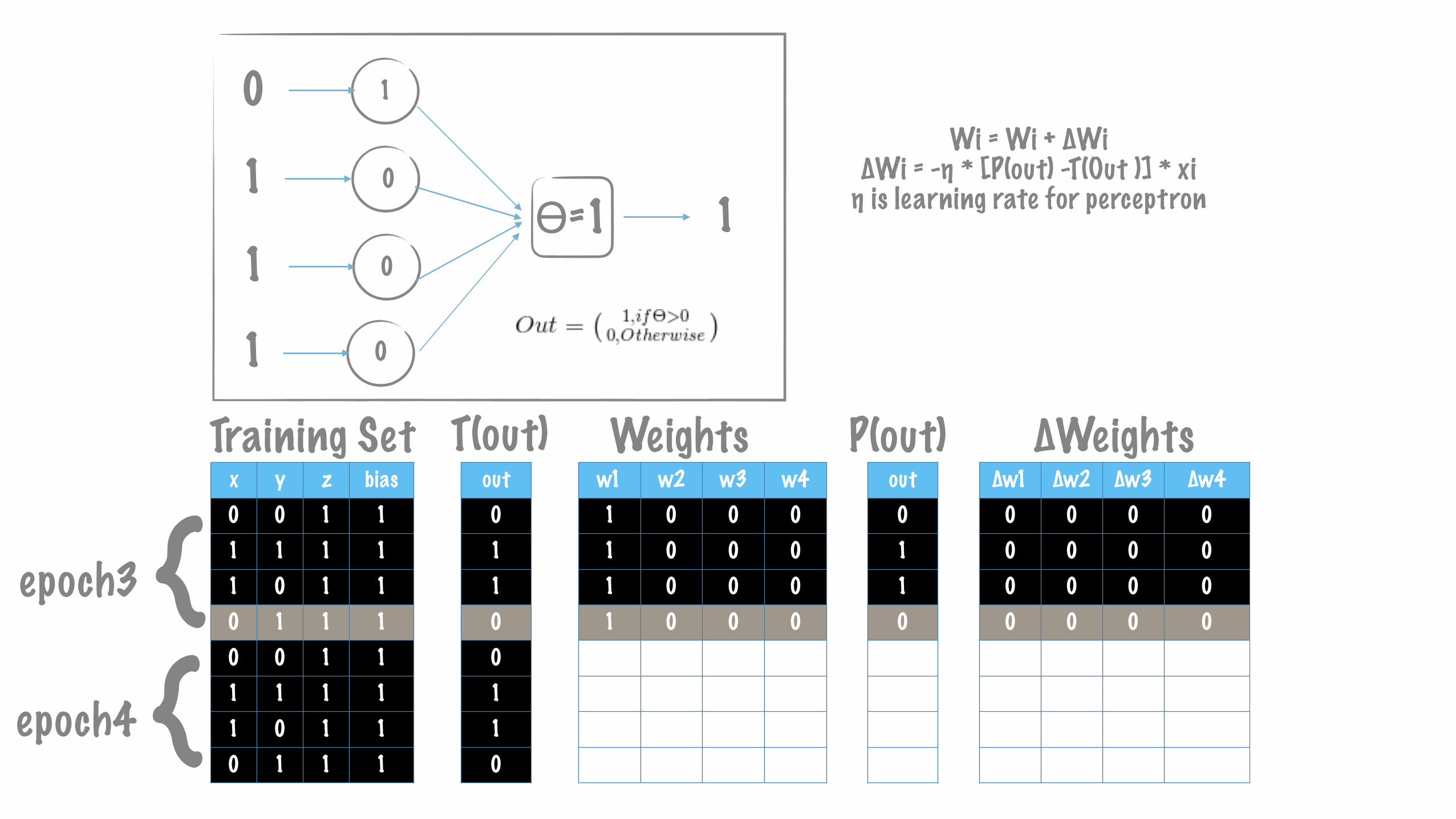
x y z bias0 0 1 11 1 1 11 0 1 10 1 1 10 0 1 11 1 1 11 0 1 10 1 1 1
∆w1 ∆w2 ∆w3 ∆w40 0 0 00 0 0 00 0 0 00 0 0 00 0 -1 -10 0 0 00 0 0 00 0 0 0
w1 w2 w3 w41 0 0 01 0 0 01 0 0 01 0 0 01 0 1 11 0 0 01 0 0 01 0 0 0
out01101110
Training Set Weights P(out) ∆Weightsout01100110
T(out)
{epoch3
1
ϴ=1 10
0
0
0
1
1
1
Wi = Wi + ∆Wi ∆Wi = -η * [P(out) -T(Out )] * xi η is learning rate for perceptron
{epoch4
∆w1 ∆w2 ∆w3 ∆w40 0 0 00 0 0 00 0 0 00 0 0 0
w1 w2 w3 w41 0 0 01 0 0 01 0 0 01 0 0 0
out0110
Training Set Weights P(out) ∆WeightsT(out)
1
ϴ Out0
0
0
x
y
z
1
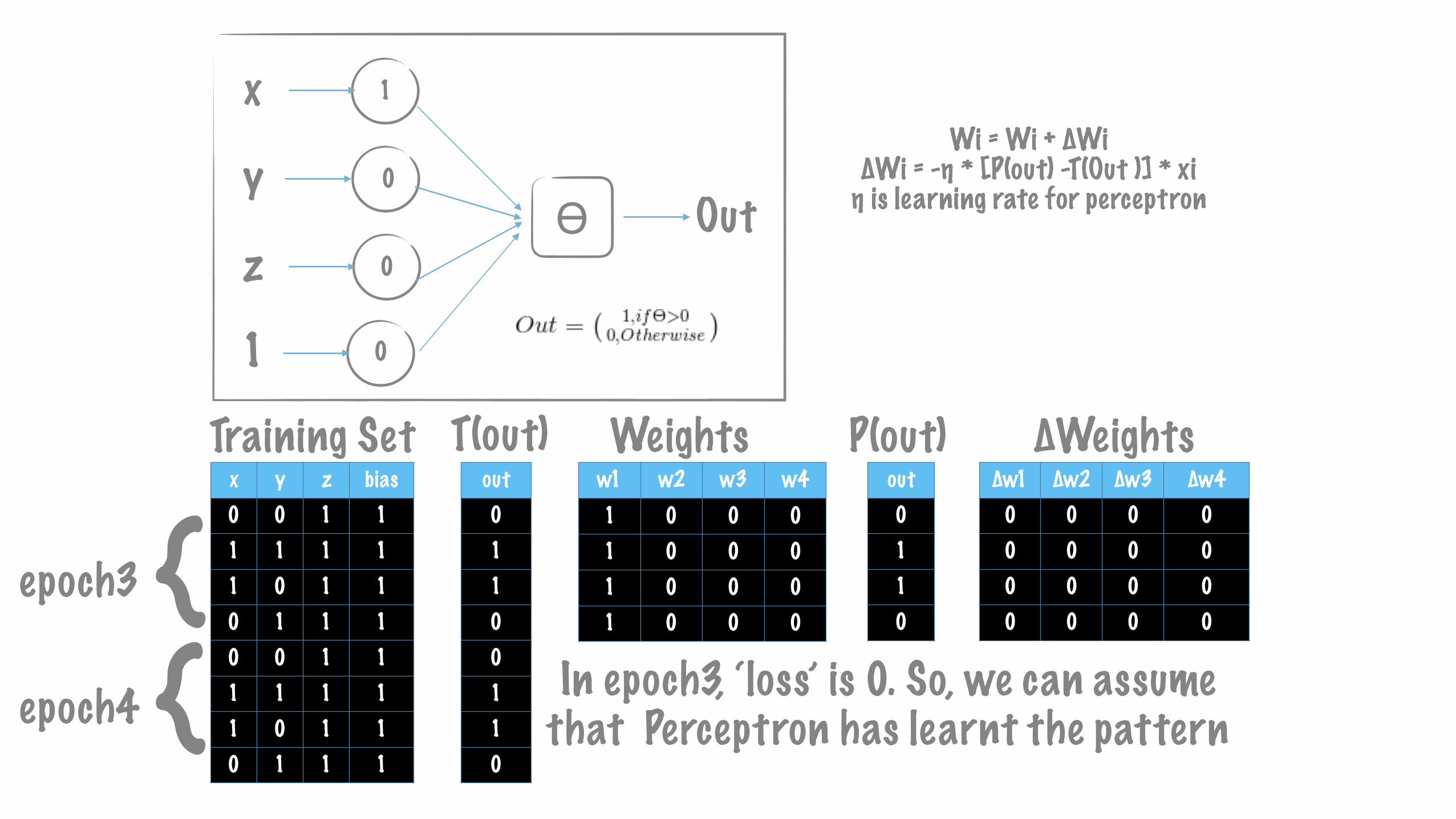
Wi = Wi + ∆Wi ∆Wi = -η * [P(out) -T(Out )] * xi η is learning rate for perceptron
{epoch3
Wi = Wi + ∆Wi ∆Wi = -η * [P(out) -T(Out )] * xi η is learning rate for perceptron
x y z bias0 0 1 11 1 1 11 0 1 10 1 1 10 0 1 11 1 1 11 0 1 10 1 1 1
out01100110
In epoch3, ‘loss’ is 0. So, we can assume that Perceptron has learnt the pattern{epoch4
We trained our Perceptron Model
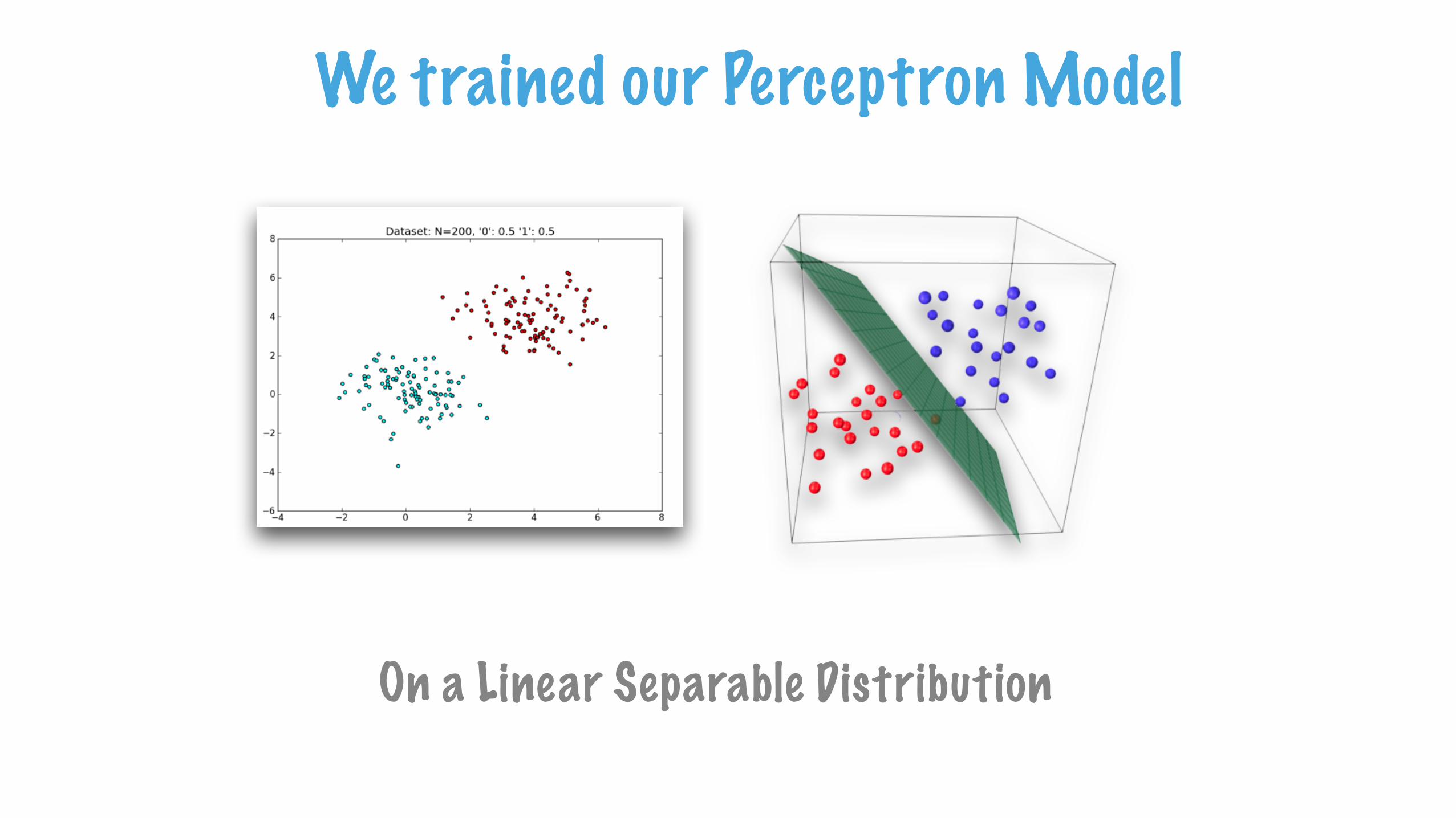
On a Linear Separable Distribution
We trained our Perceptron Model
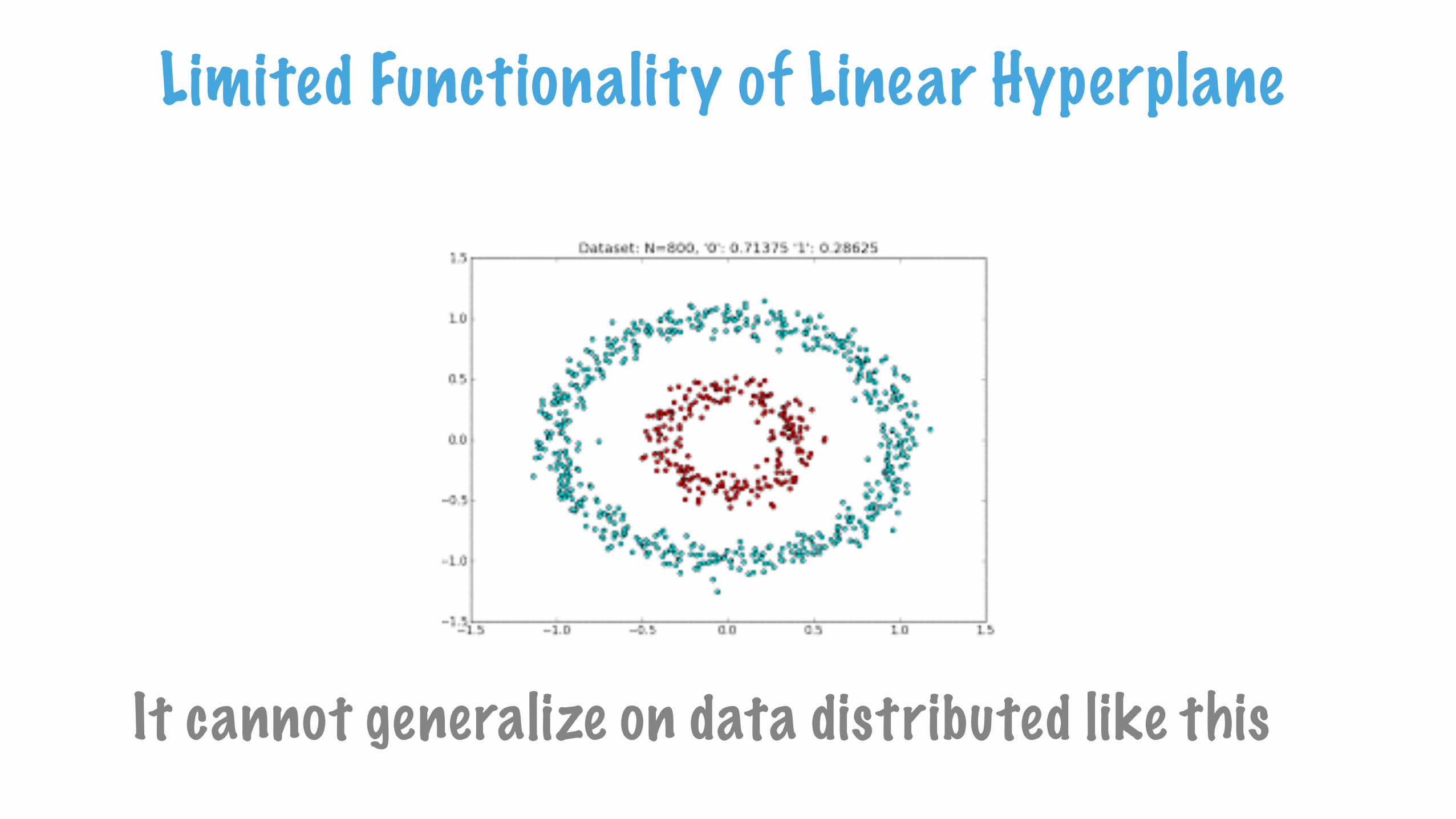
It cannot generalize on data distributed like this
Limited Functionality of Linear Hyperplane
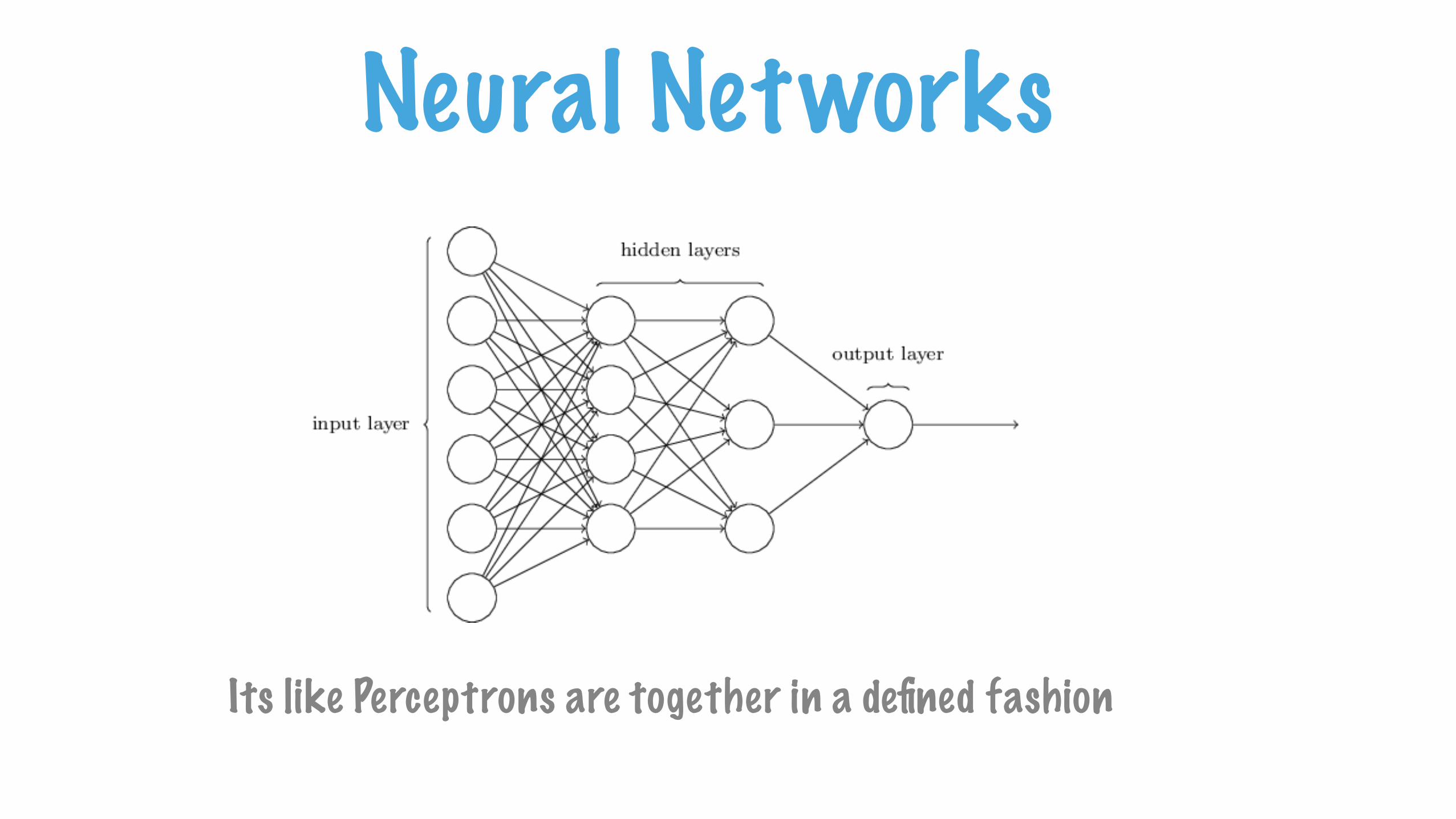
Neural Networks
Its like Perceptrons are together in a defined fashion
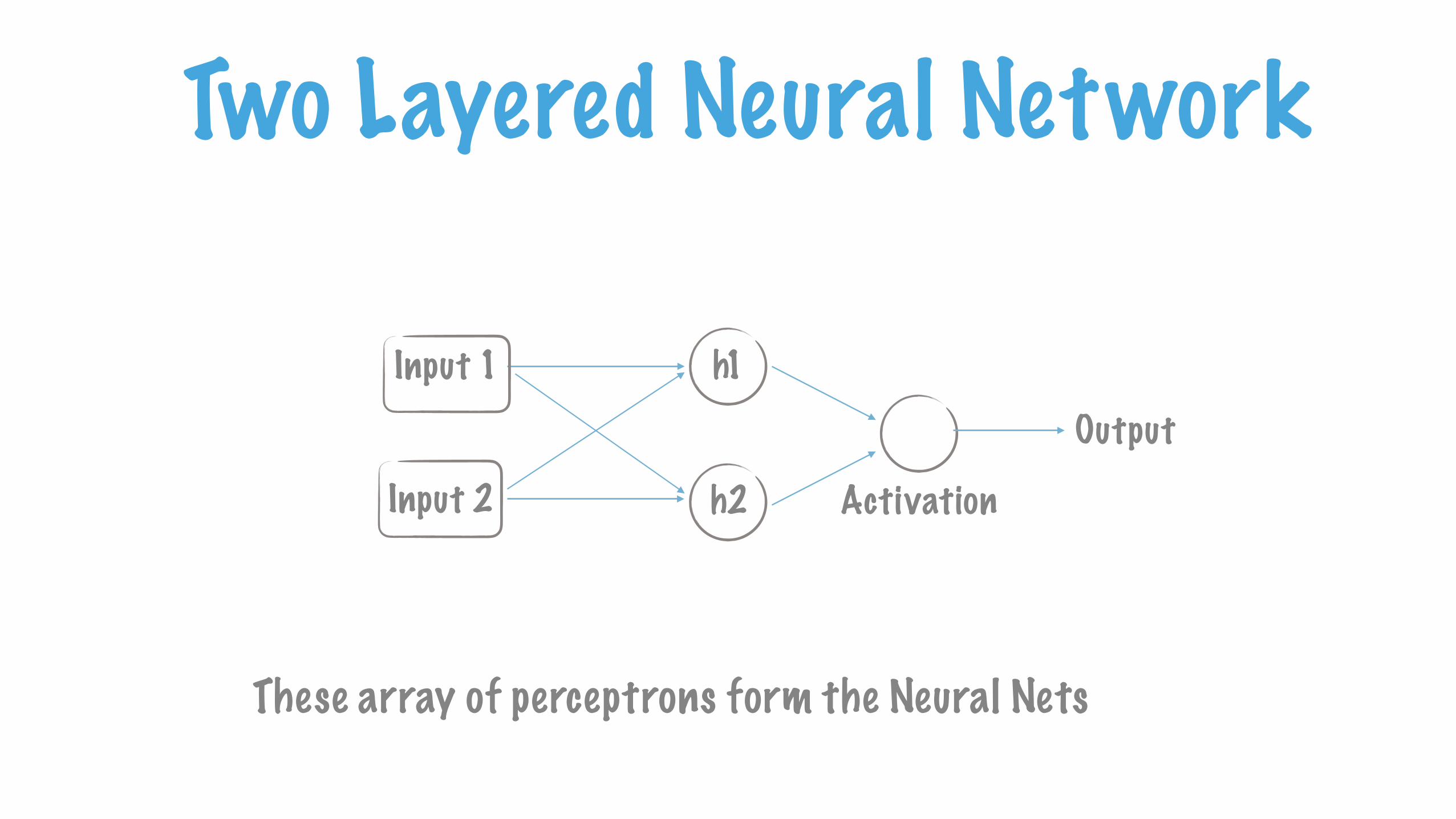
Two Layered Neural Network
These array of perceptrons form the Neural Nets
h1
h2
Input 1
Input 2Output
Activation
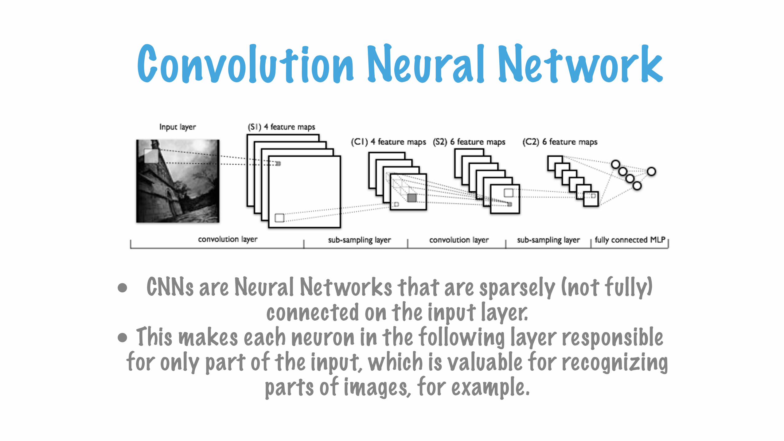
Convolution Neural Network
• CNNs are Neural Networks that are sparsely (not fully) connected on the input layer.
• This makes each neuron in the following layer responsible for only part of the input, which is valuable for recognizing
parts of images, for example.
Convolutional Neural Network
•Convolutional Neural Networks are very similar to ordinary Neural Networks
•The architecture of a CNN is designed to take advantage of the 2D structure of an input image

What is an Image ?
• Image is a matrix of pixel values • Believe me Image is nothing more than this.
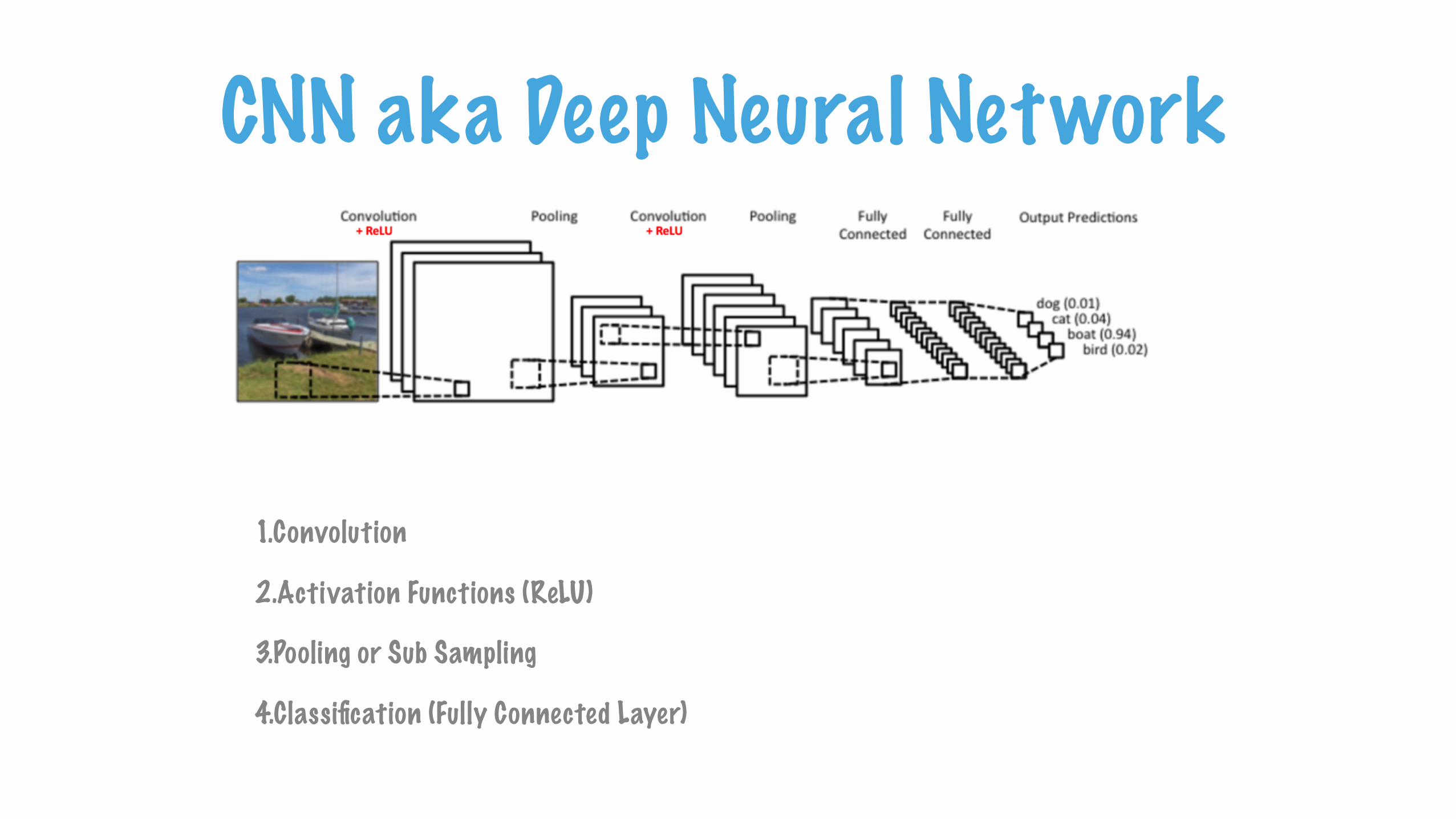
CNN aka Deep Neural Network
1.Convolution
2.Activation Functions (ReLU)
3.Pooling or Sub Sampling
4.Classification (Fully Connected Layer)
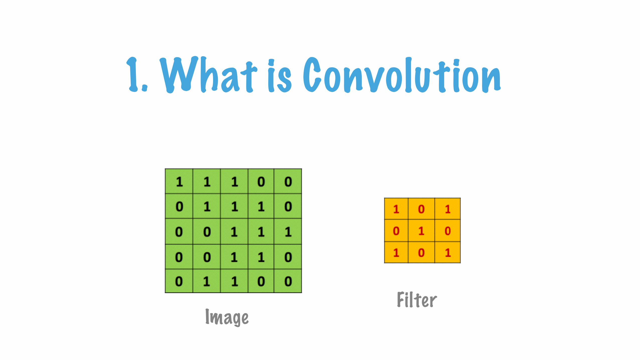
ImageFilter
1. What is Convolution
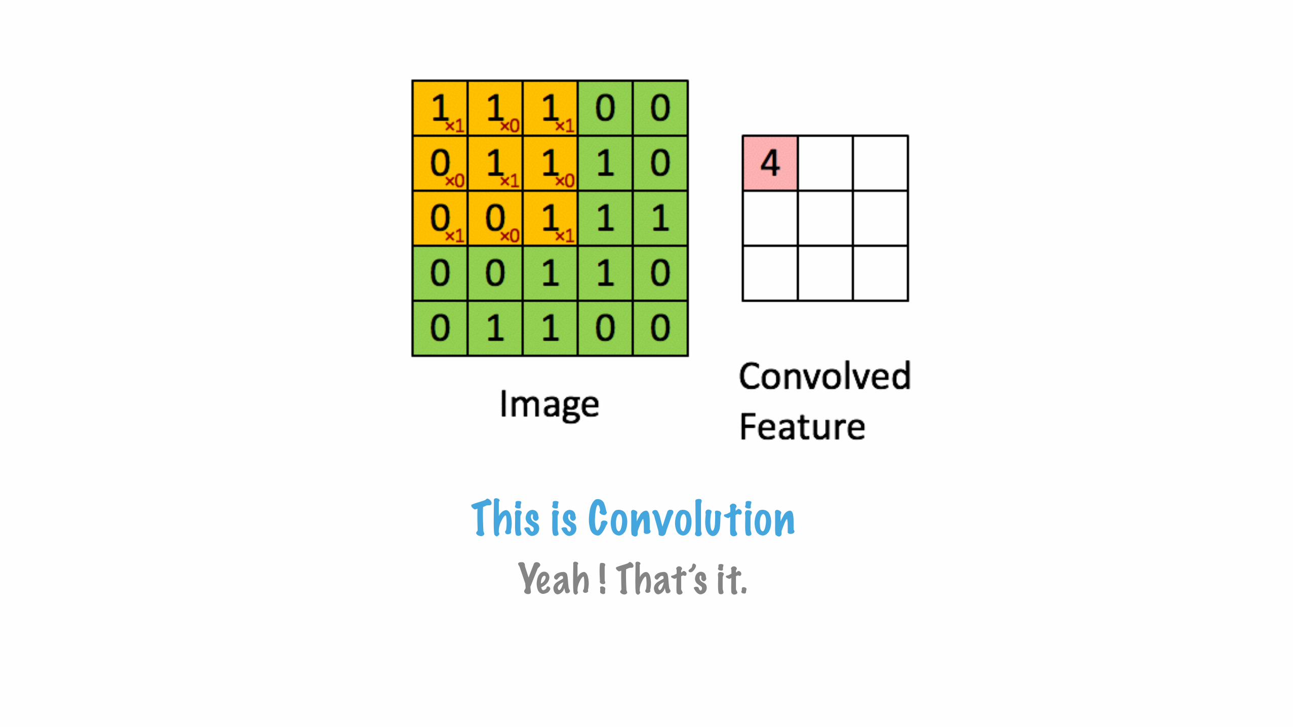
This is ConvolutionYeah ! That’s it.
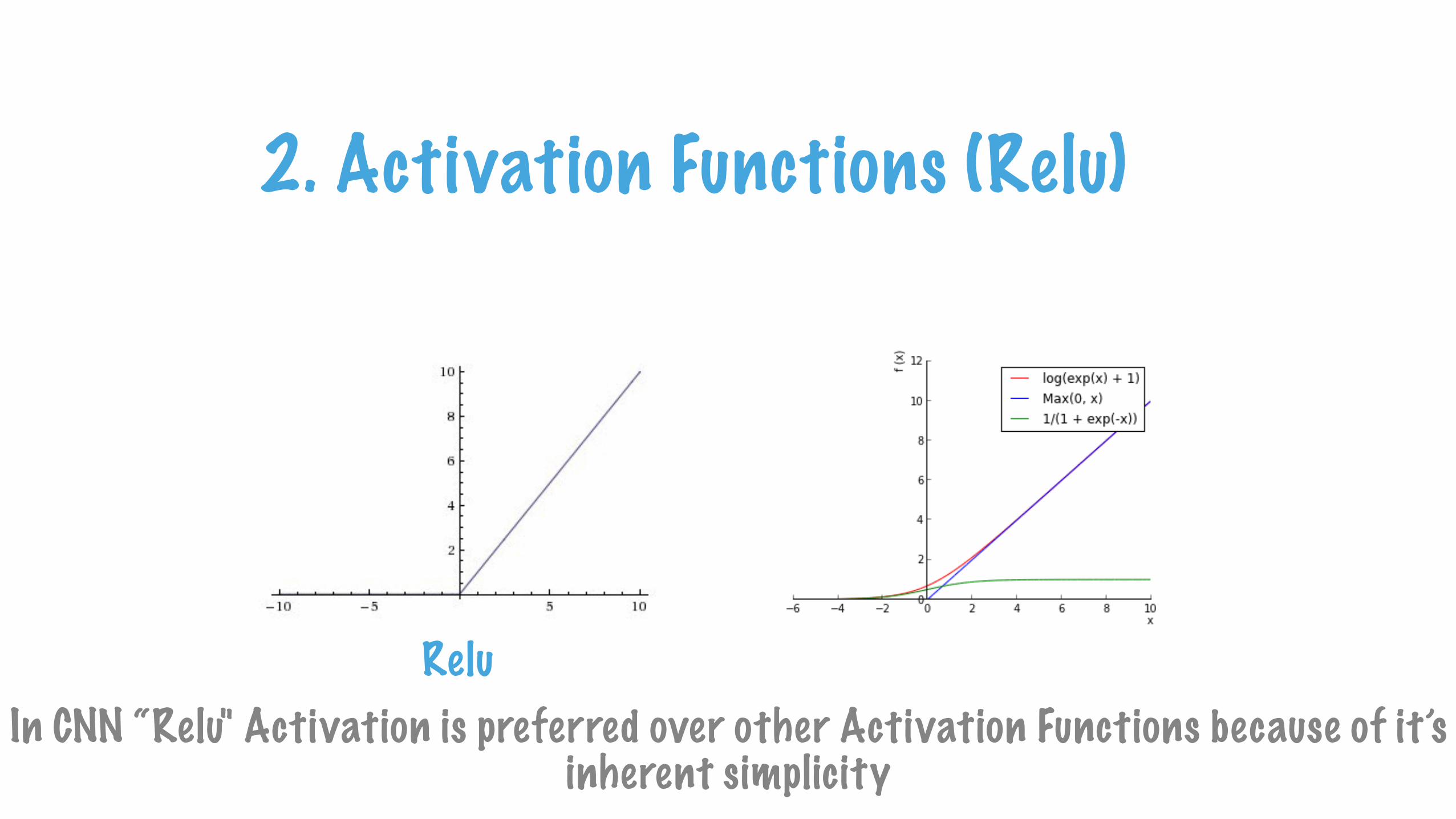
2. Activation Functions (Relu)
ReluIn CNN “Relu" Activation is preferred over other Activation Functions because of it’s
inherent simplicity
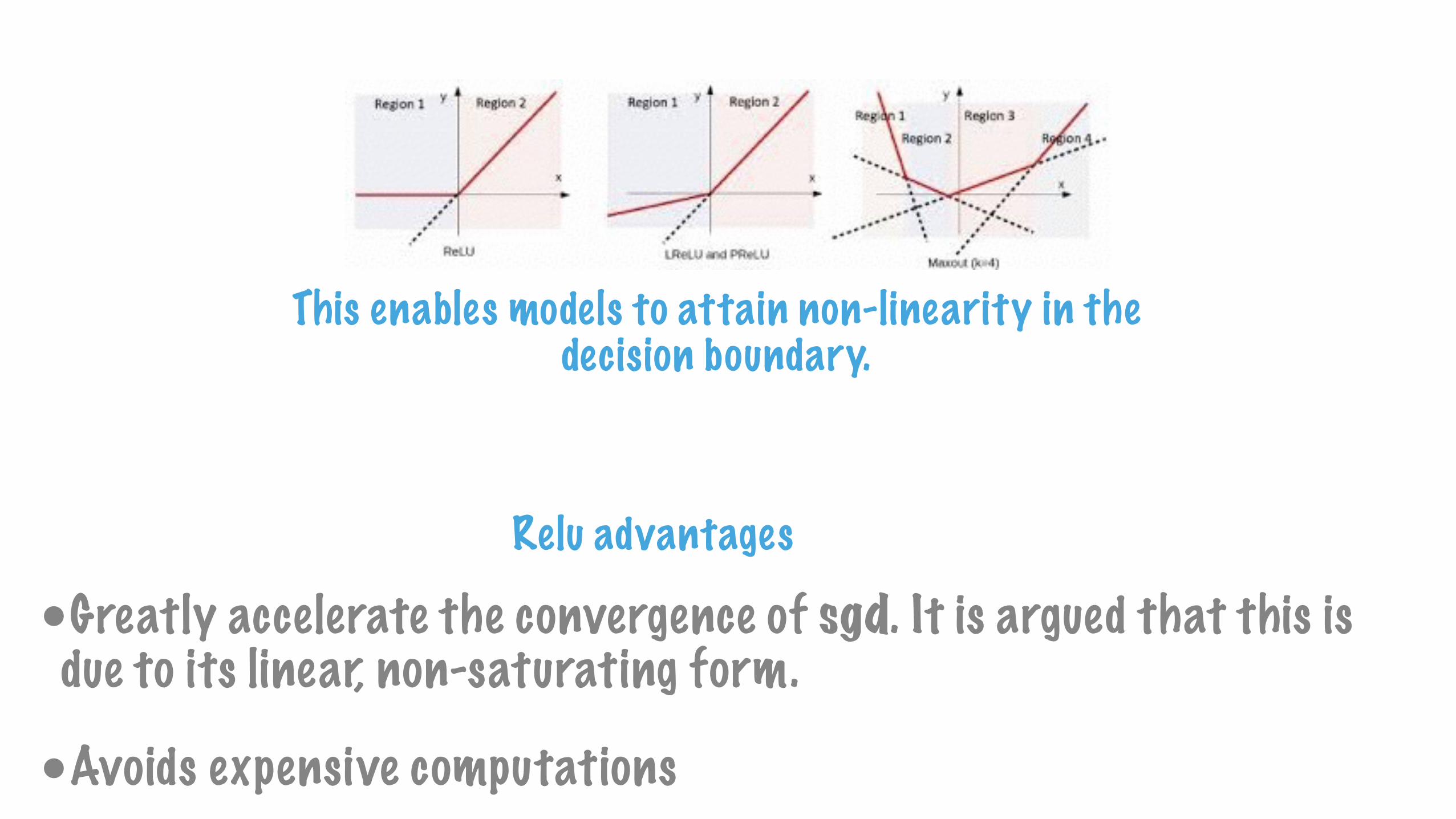
This enables models to attain non-linearity in the decision boundary.
•Greatly accelerate the convergence of sgd. It is argued that this is due to its linear, non-saturating form.
•Avoids expensive computations
Relu advantages
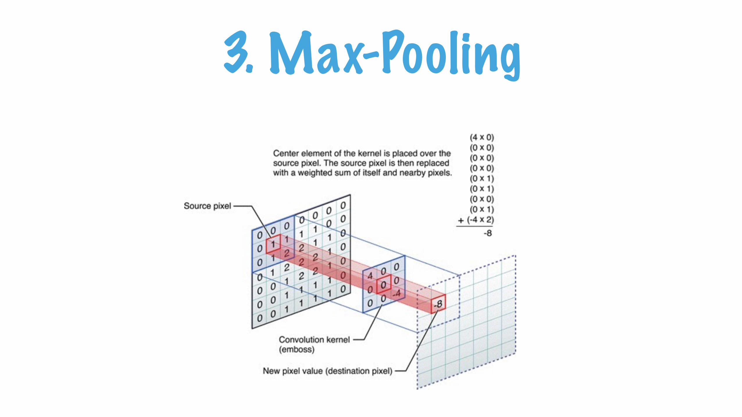
3. Max-Pooling

Pooling in Action
Spatial Pooling (also called subsampling or downsampling) reduces the dimensionality of each feature map but retains the most important information.
Spatial Pooling can be of different types: Max, Average, Sum etc.

The purpose of the Fully Connected layer is to use high-level features for classifying the input image into
various classes based on the training dataset.
4. Fully Connected Layer

Connecting dots…
1.Initialize the layers with random values.
2.The network takes a training image as input, goes through the forward propagation step (convolution, ReLU and pooling operations along with forward propagation in the Fully Connected layer) and finds the output probabilities for each class.
3.Lets say the output probabilities for the boat image above are [0.2, 0.4, 0.1, 0.3], while the target probabilities are [0, 0, 1, 0].
4.Since weights are randomly assigned for the first training example, output probabilities are also random.
5.Calculate the total error at the output layer (summation over all 4 classes.
1.Total Error = ∑ ½ (target probability – output probability) ²
6.Use Back-propagation to calculate the gradients of the error with respect to all weights in the network and use gradient descent to update all filter values / weights and parameter values to minimize the output error
•Repeat steps 2-6 with all images in the training set.
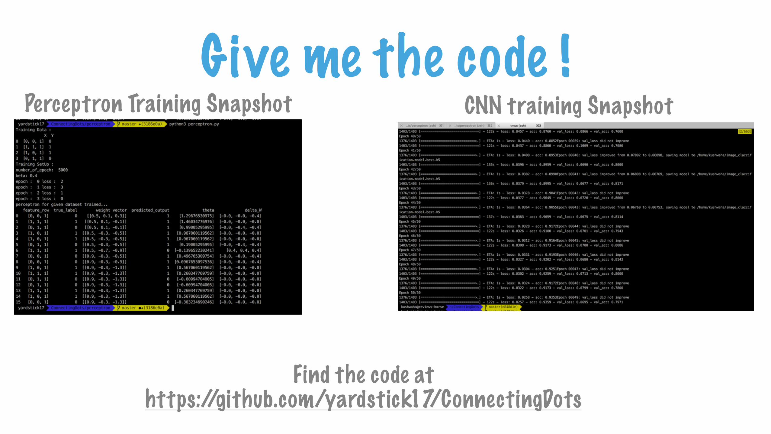
Give me the code !
Find the code at https://github.com/yardstick17/ConnectingDots
Perceptron Training Snapshot CNN training Snapshot

Thanks

References


![Convolutional Neural Networks - Cross Entropy · [IDL] Convolutional Neural Networks 1. Filters, Strides, and Padding 2. A Simple TF Convolution Example 3. Multilevel Convolution](https://img.pdfslide.net/doc/110x75/5ec609a1f93b2b072f30b881/convolutional-neural-networks-cross-entropy-idl-convolutional-neural-networks.jpg)